Relaxation dynamics of the Kondo lattice model

Abstract

We study the relaxation properties of the Kondo lattice model using the nonequilibrium dynamical mean field formalism in combination with the non-crossing approximation. The system is driven out of equilibrium either by a magnetic field pulse which perturbs the local singlets, or by a sudden quench of the Kondo coupling. For relaxation processes close to thermal equilibrium (after a weak perturbation), the relaxation time increases substantially as one crosses from the local moment regime into the heavy Fermi liquid. A strong perturbation, which injects a large amount of energy, can rapidly transform the heavy Fermi liquid into a local moment state. Upon cooling, the heavy Fermi liquid reappears in a two-stage relaxation, where the first step opens the Kondo gap and the second step corresponds to a slow approach of the equilibrium state via a nonthermal pathway.

I Introduction

Heavy Fermion compounds contain strongly interacting $f$-electrons which hybridize with extended $s$-, $p$- and $d$-electrons. The $f$-electrons are in a well-defined charge state, and at high temperature they act as local magnetic moments which scatter the conduction electrons. At low temperature, the hybridization between $f$- and conduction electrons can lead to the emergence of nontrivial electronic phases, such as the Kondo insulating state at half filling, or a strongly renormalized Fermi liquid in the doped case.Kuramoto2000 ; Coleman2007

A simple model which captures essential aspects of the physics of these materials is the Kondo lattice model.Doniach1977 In this model, charge fluctuations of the $f$-electrons are completely suppressed. The localized degrees of freedom are described by spins $S=1/2$, which are coupled to the spin of the conduction electrons at the same site via an exchange interaction $J$ (the Kondo coupling). For antiferromagnetic coupling ($J>0$), a large value of $J$ favors the formation of singlets on each site. At half-filling, this leads to the opening of a (pseudo-)gap in the spectral function of the conduction electrons. In the ferromagnetic Kondo lattice model ($J<0$), a metallic phase is realized at small coupling, with a phase transition (at half filling) to an insulating state at a critical value of $J$.Werner06Kondo

The most interesting behavior is found away from half-filling, where an antiferromagnetic interaction with the localized moments leads to a renormalized bandstructure at low temperature, which resembles a flat band hybridized with the wide band of the conduction electrons. This Fermi liquid is characterized by strong mass renormalizations and a “large” Fermi surface, i.e., both conduction electrons and localized moments participate in the formation of the Fermi liquid state, and the Luttinger volume thus contains the total number of $c$- and $f$-electrons.Oshikawa2000 As the temperature is raised or the coupling $J$ is reduced, a crossover occurs to a metallic state with a blurred, “small” Fermi surface, whose Luttinger volume contains the conduction electrons only. This physics has been beautifully demonstrated in a recent series of papers by Otsuki and collaborators, based on the dynamical mean field approximation (DMFT).Otsuki09a ; Otsuki09b

In the present paper, we use the nonequilibrium extension of DMFT to investigate the real-time dynamics of the Kondo lattice model under strong nonequilibrium conditions. In particular, we are interested in the timescales on which the system can undergo a transition between states with a large and small Fermi surface. In practice, it is easy to perturb the system so strongly that the heavy Fermi liquid is destroyed after re-thermalization at higher energy. We will implement such a perturbation by a sudden change of the interaction $J$, or a short magnetic field pulse, and investigate the crossover into the state with small Fermi surface in real time. The transition back to the heavy Fermi liquid is then achieved upon cooling, by coupling the system to a dissipative environment which absorbs the energy injected into the system by the perturbation. Although the maximal cooling rate is limited by the coupling strength, the way in which the Fermi liquid state is approached and the timescale for this process can still reveal intrinsic properties of the Kondo lattice model. To understand those relaxation times, we also consider the relaxation of the system close to equilibrium, by perturbing the local singlets with a weak magnetic field pulse. Due to the small amount of energy injected by such a weak pulse, the time evolution takes place only within one given phase and allows us to extract the equilibrium relaxation rate in the various temperature and doping regimes, and to connect this quantity to the presence or absence of strongly renormalized quasi-particles.

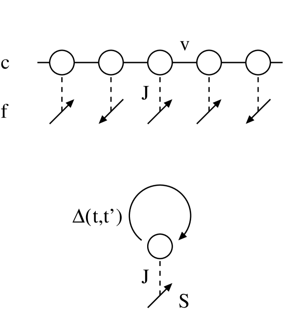
Figure 1: Top panel: illustration of the Kondo lattice model, describing conduction band electrons $c$ hopping with matrix element $v$ between orbitals (circles) and interacting via an exchange coupling $J$ with the spin of the localized $f$-electrons (arrows). Bottom panel: dynamical mean field approximation of the Kondo lattice model, consisting of one $c$-electron orbital and the associated $f$-electron spin. The $c$-electrons couple to a self-consistently determined bath of noninteracting sites, with hybridization function $\Delta(t,t^{\prime})$.

II Model and method

The spin-$\frac{1}{2}$ Kondo lattice model describes conduction electrons $c$ interacting with localized electrons $f$. If the $f$-orbitals are half-filled and fluctuations into empty or doubly occupied states are energetically very expensive, only the spin degree of freedom $\mathbf{S}=\frac{1}{2}\psi_{f}^{\dagger}\boldsymbol{\sigma}\psi_{f}$ remains in a low-energy model, while the charge fluctuations are suppressed [$\psi_{f}^{\dagger}=(f^{\dagger}_{\uparrow},f^{\dagger}_{\downarrow})$]. The Hamiltonian of the Kondo lattice model then becomes

$$H=-\sum_{i\neq j,\sigma}v_{ij}c^{\dagger}_{i,\sigma}c_{j,\sigma}+\mu\sum_{i,\sigma}n_{i,\sigma}+J\sum_{i}\boldsymbol{S}_{i}\cdot\boldsymbol{s}_{i}.$$ (1)

Here, the first term corresponds to the kinetic energy of the conduction electrons, the second term gives the chemical potential contribution of the conduction electrons ($n_{i,\sigma}=c^{\dagger}_{i,\sigma}c_{i,\sigma}$), and the last term describes the interaction of the spins $\boldsymbol{s}_{i}=\tfrac{1}{2}\psi_{c,i}^{\dagger}\boldsymbol{\sigma}\psi_{c,i}$ of the conduction electrons with the localized electrons via the Kondo coupling $J$ [$\psi_{c}^{\dagger}=(c^{\dagger}_{\uparrow},c^{\dagger}_{\downarrow})$]. In this study, we will restrict our attention to antiferromagnetic $J$ and to paramagnetic solutions.

To investigate the properties of this model, we use dynamical mean field theory (DMFT).Georges96 This approximate method, which becomes exact in the limit of infinite coordination number,Metzner89 maps the lattice model onto a self-consistent solution of a quantum impurity model. The mapping can be applied to nonequilibrium situationsSchmidt2002 ; Freericks2006 by reformulating the theory on the Keldysh time contour $\mathcal{C}$. As illustrated in Fig. 1, the impurity consists of a $c$-electron orbital coupled to a spin $\boldsymbol{S}$ and a bath of non-interacting sites. The relevant properties of the bath are encoded in the hybridization function $\Delta(t,t^{\prime})$, which describes the probability for transitions of $c$-electrons from the impurity site into the bath and back. Hence, the impurity action reads

$$\mathcal{S}=-i\int_{\mathcal{C}}\!\!dt\,H_{\text{loc}}(t)-i\int_{\mathcal{C}}\!\!dtdt^{\prime}\,\sum_{\sigma}c_{\sigma}^{\dagger}(t)\Delta(t,t^{\prime})c_{\sigma}(t^{\prime}),$$ (2)

where

$$H_{\text{loc}}=\mu(n_{\uparrow}+n_{\downarrow})+J\boldsymbol{S}\cdot\frac{1}{2}\psi_{c}^{\dagger}\boldsymbol{\sigma}\psi_{c}$$ (3)

is the local part of the Hamiltonian (1), consisting of the conduction electron orbital and the spin $\boldsymbol{S}$.

We will consider a lattice whose noninteracting density of states is semi-elliptical with bandwidth $4v$. In this case, the DMFT self-consistency becomes

$$\Delta(t,t^{\prime})=v^{2}G_{c}(t,t^{\prime}),$$ (4)

where $G_{c}(t,t^{\prime})$ denotes the $c$-electron Green function (see Appendix). We set $v=1$ as the unit of energy, and measure time in units of $v^{-1}$. The Green function $G_{c}(t,t^{\prime})=-i\langle T_{\mathcal{C}}c(t)c^{\dagger}(t^{\prime})\rangle$ must be computed numerically from the contour-ordered average $\langle...\rangle=\text{Tr}[T_{\mathcal{C}}e^{\mathcal{S}}...]/\text{Tr}[T_{\mathcal{C}}e^{\mathcal{S}}]$, using the action defined in Eq. (2) ($T_{\mathcal{C}}$ is the time-ordering operator on the Keldysh contour $\mathcal{C}$).

For equilibrium calculations, several techniques are available to solve the impurity problem, among them the numerical renormalization groupBulla2008 and continuous-time Monte Carlo methods.solver_review The latter come in two variants, the weak-coupling CT-J solverOtsuki07 and the hybridization expansion approach (CT-HYB).Werner06Kondo In a CT-J simulation, the partition function of the impurity model is expanded in powers of $J$, so that the Monte Carlo configurations consist of arbitrary sequences of spin-flip processes, with weight proportional to a determinant of a matrix of bath Green functions. In a CT-HYB calculation, the local problem $H_{\text{loc}}$ is solved exactly, while the expansion of the partition function is done in powers of the hybridization function $\Delta$. Here, the weight is proportional to the determinant of a matrix of hybridization functions.

Neither CT-J nor CT-HYB suffers from a sign problem in equilibrium calculations. Monte Carlo simulations on the real-time Keldysh contour, however, lead to a dynamical sign problem,Werner09 ; Werner10 which restricts the simulations to rather short times. Since we are interested in both the transient dynamics of the Kondo lattice model and the long-time relaxation towards an equilibrium state, we use the non-crossing approximation (NCA) as an impurity solver. Similar to CT-HYB, NCA is based on an expansion of the impurity partition function in powers of the hybridization functions. But rather than combining various (crossing and non-crossing) diagrams into a determinant, only the non-crossing diagrams are retained and summed up analytically via a Dyson equation. The implementation of the NCA impurity solver on the Keldysh contour has been explained in Ref. Eckstein10nca, , and we use the same procedure with the local Hamiltonian $H_{\text{loc}}$ represented as a $8\times 8$ block matrix in the basis $|S;n_{\uparrow};n_{\downarrow}\rangle$, with $S=\uparrow,\downarrow$ and $n_{\sigma}=0,1$. Other formulations of (extendend) NCA for the Kondo lattice model have been previously used.Pruschke1995 An advantage of the present formulation with an $8$-dimensional local problem is that it captures the formation of local singlets at the $0$th order of the approximation.footnote00 The NCA solver does not suffer from a sign problem, so that the computational effort grows polynomially (like the third power) with the maximum simulation time. We converge the DMFT equations on the real-time contour time-step by time-step, using the procedure detailed in Ref. Eckstein10quench, .

In order to characterize the various equilibrium and nonequilibrium phases, we compute both static observables, such as the momentum distribution, and the frequency dependent spectral function. For a general time-evolving state, the latter can be defined as

$$A(\omega,t)=-\frac{1}{\pi}\text{Im}\int_{t}^{\infty}dt^{\prime}e^{i\omega(t^{\prime}-t)}G^{\text{ret}}(t^{\prime},t),$$ (5)

where $G^{\text{ret}}(t,t^{\prime})=-i\Theta(t-t^{\prime})\langle\{c(t),c(t^{\prime})\}\rangle$ is the retarded Green function. In practice, the time-integral is limited to some maximal time $t^{\prime}=t_{\text{max}}$, which could lead to artificial oscillations in the results. Below, this effect is well controlled with a suitably large cutoff $t_{\text{max}}\approx 50$.

In principle, there is always some arbitrariness in the definition of a nonequilibrium spectral function, and in general, the Fourier transform Eq. (5) need not even be positive. However, in particular when the inverse width of the spectral features is small compared to the timescale on which $A(\omega,t)$ changes, the function (5) is closely related to a time-resolved photoemission and inverse photoemission spectrum.TRPES Moreover, $A(\omega,t)$ constitutes a complete representation of the local Green function, and for an equilibrium state $A(\omega)\equiv A(\omega,t)$ becomes time-independent and reduces to the conventional definition.

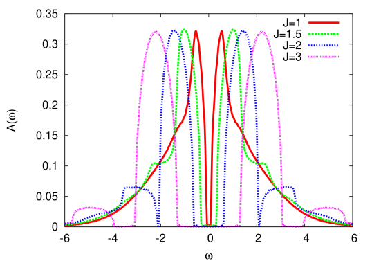
Figure 2: Spectral functions of the $n_{c}=1$ Kondo insulator at $\beta=50$ and indicated values of $J$.

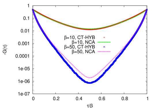
Figure 3: Comparison between Green functions from CT-HYB and NCA for $J=1.5$, $n_{c}=1$, and indicated temperatures.

III Results

III.1 Equilibrium properties

In order to set the stage for the study of the relaxation dynamics and to test the quality of the NCA approximation, we first compute various results for the Kondo lattice model in equilibrium. Figure 2 shows the conduction electron spectral function (5) at half-filling ($\mu=0$, $n_{c}=1$), for several values of $J$ and inverse temperature $\beta=50$. For sufficiently low temperature, the singlet formation between the conduction-electron and localized spins leads to the opening of a gap (Kondo insulator). The separation between the peaks is given by $E(n=2)+E(n=0)-2E(n=1)=1.5J$, where $E(n=0)=0$, $E(n=1)=-\frac{3}{4}J-\mu$ and $E(n=2)=-2\mu$ are the lowest energy states for the local problem ($H_{\text{loc}}$) with $n$ $c$-electrons.Werner06Kondo The side-peaks which are split off by $J$ correspond to the insertion or removal of an electron with additional singlet-triplet excitations. Due to the exponential decay of the hybridization function in the Kondo insulating phase, we expect the NCA approximation to be rather accurate in this regime.Gull2010 ; Eckstein10nca As shown in Fig. 3, already for $J=1.5$ the NCA solution indeed provides a good approximation of the exact Green function, although NCA slightly underestimates the size of the Kondo gap, in contrast to the Mott gap in the Hubbard model.Eckstein10nca

As one dopes the system, a narrow quasi-particle peak appears near the Fermi level at low temperatures. Figure 4 shows spectral functions for $J=1.5$, $n_{c}=1.1$ and $n_{c}=1.4$, and different inverse temperatures $\beta$. As the temperature is increased, the narrow feature disappears ($\beta=10$), but the Fermi level remains at the upper edge of the partially filled-in Kondo insulator gap. Eventually, the upper gap edge moves away from the Fermi level ($\beta=5$) and at even higher temperatures ($\beta=2$), the gap starts to fill in. At larger doping, the pseudo-gap is less pronounced and the low-temperature quasi-particle peak is merged with the upper band.

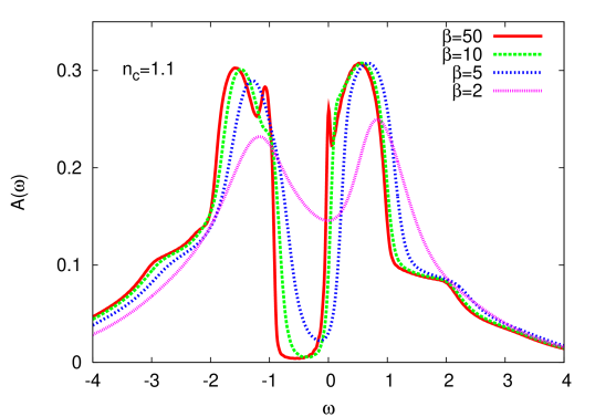
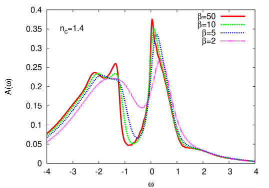
Figure 4: $J=1.5$. Temperature-dependence of the spectral function for $n_{c}=1.1$ (top panel) and $n_{c}=1.4$ (bottom) panel.

To get a better understanding of the crossover between the various phases, we plot in Fig. 5 the temperature-dependence of the real part of the conduction electron self-energy at frequency $\omega=0$, $\text{Re}\Sigma(0)$, and the occupation $p_{\text{singlet}}$ of the impurity singlet state ($p_{\text{singlet}}=\langle P_{1}(\tfrac{1}{4}-\boldsymbol{s}\cdot\boldsymbol{S})\rangle$, where $P_{1}=n_{\uparrow}+n_{\downarrow}-2n_{\uparrow}n_{\downarrow}$ is the projector on the one-particle sector of the local Hilbert space). The behavior of $\text{Re}\Sigma(0)$ was used in Ref. Otsuki09a, to define the crossover scale $T^{*}$ below which a coherent Fermi liquid state is formed. The evolution of $\text{Re}\Sigma(0)$ in our case looks similar to what was found in Ref. Otsuki09a, for a hypercubic lattice, and the temperature dependence is also qualitatively consistent with the numerically exact CT-HYB results for the semi-circular DOS. We have used a linear extrapolation procedure to estimate $\text{Re}\Sigma(0)$ from the values $\Sigma(i\omega_{n})$ at non-zero Matsubara frequencies, rather than the quadratic fit employed in Ref. Otsuki09a, , because this seems more appropriate at the relatively high temperatures considered in this study. At the filling $n_{c}=1.1$, the heavy Fermi liquid appears below $T^{*}\approx 0.1$, so that we can associate the shift of the Fermi level in Fig. 4 from a position within the (pseudo-)gap into the upper band and the formation of a narrow resonance with the appearance of heavy quasi-particles and the formation of the large Fermi surface. Comparison with the temperature dependence of $p_{\text{singlet}}$ shows that the enhanced singlet formation sets in already at a higher temperature, below a crossover scale $T_{K}\approx 0.5$. Hence there is a temperature range $T^{*}<T<T_{K}$ between the Fermi liquid and local moment regime, where the singlet formation leads to a pronounced pseudo-gap in the spectral function and the Fermi level lies inside this gap. Above $T_{K}$, $p_{\text{singlet}}$ decreases and the pseudogap in the spectral function starts to fill in. The existence of the two temperature scales $T^{*}$ and $T_{K}$ in the single-site DMFT solution of the Kondo lattice model has been previously discussed in Ref. Burdin00, . The crossover temperatures are correctly reproduced by the NCA approximation and, at least in the range considered here, they show little dependence on doping.

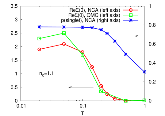
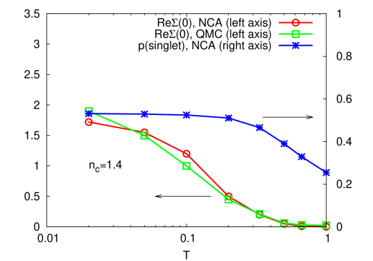
Figure 5: $J=1.5$. Temperature dependence of the extrapolated value $\text{Re}\Sigma(0)$ (left axis), showing the crossover from the Kondo insulator regime to the Fermi liquid regime below $T^{*}$. Also plotted is the temperature dependence of the occupation of the singlet state (right axis), which illustrates the crossover from the local moment regime at high $T$ to the Kondo insulator regime below $T_{K}$. The top panel shows data for $n_{c}=1.1$ and the bottom panel for $n_{c}=1.4$.

The most direct evidence for a large Fermi surface is obtained from the momentum distribution $n(\epsilon)$, which is given by the expectation value $\langle c_{\boldsymbol{k}}^{\dagger}c_{\boldsymbol{k}}\rangle$ for band energy $\epsilon=\epsilon_{\boldsymbol{k}}$ (see Appendix). It is shown in Fig. 6 for different couplings $J$ at $\beta=50$ and $n_{c}=1.1$, and $1.4$. At small values of $J$, a smeared-out step is visible around the location of the Fermi surface of a free conduction electron gas. The formation of the heavy quasi-particle band leads to a step in the distribution function $n(\epsilon)$ at a different location and with a smaller size, corresponding to a shift of the Fermi surface and a reduction of the quasiparticle weight.

We conclude from these results that our NCA approximation, which exactly treats an 8-dimensional local problem, provides a qualitatively correct description of the Kondo insulator, the heavy Fermi liquid and local moment regimes in the doped model, and of the various crossover phenomena. In the following, we will use this approach to study the relaxation properties of the Kondo lattice model in the different parameter regimes.

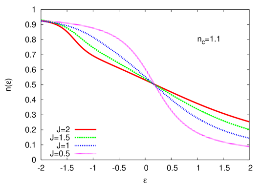
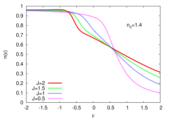
Figure 6: Distribution function $n(\epsilon)$ for the antiferromagnetic Kondo lattice model at $\beta=50$. The top panel corresponds to a filling $n_{c}=1.1$ and the bottom panel to $n_{c}=1.4$. For large $J$, one observes the formation of a small kink in $n(\epsilon)$, corresponding to the large Fermi surface, where the heavy quasiparticle band crosses the Fermi energy.

III.2 Relaxation close to thermal equilibrium

We next compute the relaxation times of the system after it is weakly perturbed in one of the various parameter regimes discussed above. This will later on be important to understand the behavior of the system after a strong perturbation, for times long enough that a new equilibrium state is approached. The relaxation times are still entirely determined by equilibrium properties of the corresponding electronic phase, which is not left by the weak perturbation. Technically, the following investigation could thus be done by computing a suitable linear response quantity within the Matsubara formalism, but it is more convenient to do an explicit real-time calculation, which avoids analytical continuations and also does not require the evaluation of vertex functions of the impurity model.

Specifically, we consider the relaxation of the system after a short and weak magnetic field pulse, which acts only on the localized spin by means of an additional perturbation $h_{x}(t)S_{x}$ in the Hamiltonian (3). The pulse is of the form

$$h_{x}(t)=h\sin^{2}(\pi t/t_{\text{pulse}})$$ (6)

for $t<t_{\text{pulse}}$ and $h_{x}(t)=0$ for $t>t_{\text{pulse}}$. We use pulses of duration $t_{\text{pulse}}=1.5$ and small field strength $h$, such that the heating effect is comparatively weak and we can study the relaxation time within the three temperature regimes $T<T^{*}$ (“Fermi liquid”, FL), $T^{*}<T<T_{K}$ (“Kondo insulator”, KI) and $T>T_{K}$ (“local moment”, LM). We will focus on the time evolution of $p_{\text{singlet}}$. Other observables, such as the double-occupancy on the $c$-site, or the distribution function $n(\epsilon,t)$ seem to give consistent results for the relaxation time.

Because the pulse is acting only on one of the two spins which form the singlet (the localized spin $\boldsymbol{S}$), it perturbs the singlet and leads to an initial decrease in $p_{\text{singlet}}$. This decrease is followed by a complicated transient evolution up to about $t\approx 10$, after which the system eventually settles into an exponential relaxation towards a new thermal equilibrium state at somewhat higher temperature. To measure the relaxation time $\tau$, we fit this long-time behavior with an exponential function $p_{\text{singlet}}(t)=p_{\text{singlet}}(t=\infty)+A\exp(-t/\tau)$. For several sets of parameters we have cross-checked that within the accuracy of our calculation the extrapolated final value $p_{\text{singlet}}(t=\infty)$ obtained from the fit corresponds to the value computed independently by assuming thermalization at constant energy.

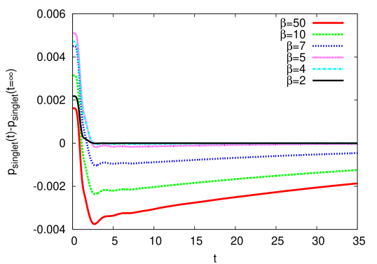
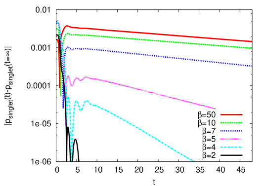
Figure 7: Relaxation of $p_{\text{singlet}}$ after a $h$-field pulse of strength $h=0.1$, as a function of temperature. The initial state is the equilibrium state for indicated temperatures, $n_{c}=1.1$, $J=1.5$. After the pulse, the system with $\beta=50$ relaxes to a thermal state with inverse temperature $\approx 15$, and the system with $\beta=5$ to a thermal state with inverse temperature $\approx 4.8$.

Figure 7 shows the time-evolution of $p_{\text{singlet}}(t)-p_{\text{singlet}}(t=\infty)$ after a pulse of strength $h=0.1$ and duration $t_{\text{pulse}}=1.5$, for $J=1.5$ and $n_{c}=1.1$. The initial state is the equilibrium state at different temperatures. In the FL regime ($T\lesssim 0.1$), the transient is relatively smooth, and the exponential relaxation towards the equilibrium state becomes remarkably slow. In the KI regime $1/7\lesssim T\lesssim 1/3$, three things happen: (i) the transient exhibits a plateau with oscillations whose period is roughly proportional to $1/J$, (ii) the exponential relaxation becomes substantially faster with increasing temperature, and (iii) the exponential relaxation sets in from a value of $p_{\text{singlet}}$ which is much closer to the thermal value than in the FL regime. Finally, in the LM regime, the relaxation is so fast that after the initial transient (which seems to take about $t\approx 10$, independent of temperature), the system has already thermalized. Within the accuracy of our simulation, it then no longer makes sense to fit an exponential to the long-time evolution.

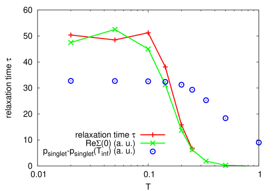
Figure 8: Relaxation time $\tau$ after a $h$-field pulse of strength $0.1$, as a function of temperature. The initial state is the equilibrium state for the indicated temperatures and $n_{c}=1.1$, $J=1.5$. For comparison, we also plot $\text{Re}\Sigma(0)$ and $p_{\text{singlet}}$ (with arbitrary rescaling).

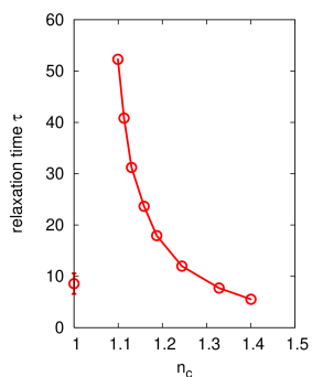
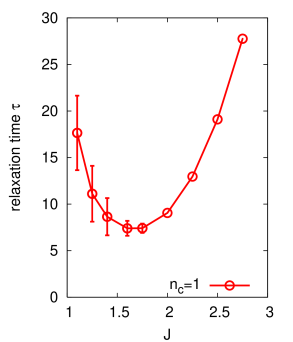
Figure 9: Relaxation time $\tau$ for $J=1.5$ as a function of doping (left panel) and at half-filling as a function of $J$ (right panel). The initial state is the equilibrium state at $\beta=50$. The large error bars at small $J$ are due to the appearance of oscillations on top of the exponential relaxation.

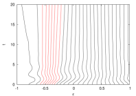
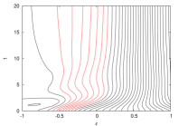
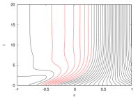
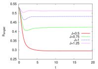
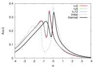
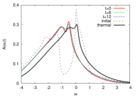
Figure 10: Top panels: Time evolution of the distribution function $n(\epsilon,t)$ after a quench from $J=1.5$, $n_{c}=1.4$, $\beta=50$ to $J=1.25$, $0.75$ and $0.5$ (from left to right). The plots show contours of constant $n$, with red contours corresponding to values of $\epsilon$, which in the initial state are associated with the large Fermi surface discontinuity. Bottom left panel: Time evolution of $p_{\text{singlet}}$. Middle panel: Time evolution of the spectral function after a quench to $J=0.75$. After thermalization, the system is in the KI phase ($\beta\approx 12.5$). Right panel: Time evolution of the spectral function after a quench to $J=0.5$ (effective temperature $\beta\approx 8.3$, in the LM phase).

The behavior in Fig. 7 is reminiscent of the relaxation dynamics found after an electric field pulse in the Hubbard model, as one approaches the insulator-metal crossover regime from the Mott insulating side.Eckstein11pump In the doped Kondo lattice model, however, the slow relaxation occurs in the heavy Fermi liquid regime, while the KI regime with a deep pseudo-gap is associated with faster relaxation.

In fact, it is the disappearance of coherent quasi-particles, and not the filling-in of the pseuo-gap, which leads to the faster relaxation. To illustrate this, we plot in Fig. 8 the relaxation time as a function of temperature, and compare this curve to $\text{Re}\Sigma(0)$ and $p_{\text{singlet}}$. The relaxation time tracks $\text{Re}\Sigma(0)$ (associated with the formation of the heavy Fermi liquid with a large Fermi surface) and not $p_{\text{singlet}}$ (associated with the opening of the gap). Furthermore, the relaxation time decreases if the Fermi liquid is weakened, for example by increasing the doping (left panel of Fig. 9). That increasing doping leads to a weakening of the heavy Fermi-liquid state is indicated by the evolution of $\text{Re}\Sigma(0)$ shown in Fig. 5, which shows that the FL state is formed at lower temperature for $n_{c}=1.4$ than for $n_{c}=1.1$, and by the spectral functions in Fig. 4, which show that the Kondo gap gets filled in with increasing doping. In the exhaustion limit $n_{c}\rightarrow 2$, the Fermi liquid coherence temperature $T^{*}$ should drop to zero.Burdin00

At least in the case $J=1.5$ considered here, the Kondo insulator relaxes much faster than the weakly doped FL (about the same relaxation time as in the weakly doped model in the KI regime above $T^{*}$). For smaller couplings, the relaxation time of the insulator increases rapidly (right panel of Fig. 9), since in the small-$J$ limit the slowest processes are $\sim 1/J$. In the limit of large $J$, the relaxation time grows because it becomes difficult to transform an excitation energy of order $J$ into kinetic energy.

III.3 Fast melting of the large Fermi surface

In this section, we study the dynamical evolution of the heavy Fermi liquid with a large Fermi surface into a state with small Fermi surface. This process can easily be triggered in many ways, provided a sufficient amount of energy is injected into the system. We will suddenly reduce the Kondo coupling $J$, which both leads to a considerable heating of the system and weakens the local singlets. The two effects combined are expected to result in a crossover from the FL phase into the KI and LM regimes. Figure 10 shows contour plots of the momentum occupation $n(\epsilon,t)$ after a quench from $J=1.5$, $\beta=50$, $n_{c}=1.4$ to $J_{\text{final}}=1.25$, $0.75$ and $0.5$. The small quench ($J_{\text{final}}\!=\!1.25$) leads to a minor shift and a thermal broadening of the large Fermi surface (indicated by the red contour lines). The slow drift of the contour lines indicates that the relaxation time is slow, as expected for relaxation processes within the FL regime. The quench to $J_{\text{final}}=0.75$ drives the system into the KI regime, where Fermi liquid coherence is lost (with a corresponding shift in $\text{Re}\Sigma(0)$), but the Kondo gap is still present. The relaxation is faster, in accordance with the faster dynamics measured after a weak magnetic field pulse in this regime. Finally, the quench to $J_{\text{final}}=0.5$ brings the system into the LM regime, characterized by a small Fermi surface. Melting of the large Fermi surface and steepening of the momentum distribution around the location of the small Fermi surface happen on the timescale of a few inverse hoppings, comparable to the relaxation time after weak perturbations within the LM phase. We observe no additional bottleneck connected to the destruction of the large Fermi surface when hopping and $J$ are comparable in magnitude.

The evolution of the system into the KI and LM phases is also evident from the behavior of $p_{\text{singlet}}$ and the shift of $\text{Re}\Sigma$. Despite the heating effect, $p_{\text{singlet}}$ remains large after quenches to $J=1.25$ and $J=1$, and the crossover into the LM regime is evident in the form of a substantial drop of $p_{\text{singlet}}$ for $J=0.5$ (lower left panel of Fig. 10). The shift of $\text{Re}\Sigma$, on the other hand is evident in the bottom right two panels (corresponding to the quenches to $J=0.75$ and $J=0.5$): A time-dependent shift of $\text{Re}\Sigma(0)$ is equivalent to a shift of the chemical potential $\mu$. In nonequilibrium DMFT calculations, a sudden shift of $\mu$ by $\Delta\mu$ results in a rigid shift of the spectral function (5) by $-\Delta\mu$ on the frequency axis. In the present case, the rapid decrease of $\text{Re}\Sigma(0)$ leads to a shift of the quasi-particle peak by $+\Delta(\text{Re}\Sigma(0))<0$. Thermalization of the spectral function is seen to occur approximately on the same time-scale as the momentum distribution function.

III.4 Formation of the heavy Fermion state upon cooling

Finally, let us consider the dynamical formation of the FL state out of the LM phase. In general, it is not possible to reach the FL phase from the LM phase by a sudden increase of $J$, since the strong heating caused by such a quench would destroy the Fermi liquid coherence. We will thus approach the problem in a different way, which is at the same time closer to possible experiments on heavy-Fermion materials. In such an experiment, one might rapidly destroy the FL phase by a strong excitation (see Sec. III.3), and monitor its reappearance out of the excited LM phase while energy is dissipated from the electronic system to the environment. As long as the intrinsic thermalization times of the system are fast compared to this dissipation time, the system will evolve through a sequence of equilibrium states of decreasing temperature, at a rate that is set by the coupling to the environment. However, when the thermalization time becomes long, the system will fall out of equilibrium, or experience a slowdown of the cooling dynamics. Since our investigation in Sec. III.2 has demonstrated a large increase of the thermalization times in the low-tempeature FL phase, one might expect the cooling dynamics in the doped Kondo lattice to reveal such a nontrivial time evolution. In the following, we will excite the system with a strong magnetic field pulse (6), and look at the subsequent dynamics in the presence of an additional particle reservoir at fixed temperature.

To model dissipation of energy to other degrees of freedom we couple a thermal particle reservoir with inverse temperature $\beta$ locally to each site of the lattice. Technically, this corresponds to a change of the DMFT self-consistency condition from Eq. (4) to

$$\Delta(t,t^{\prime})=v^{2}G_{c}(t,t^{\prime})+\Delta_{\beta}(t,t^{\prime}),$$ (7)

where the hybridization function of the reservoir is given by

$$\Delta_{\beta}(t,t^{\prime})=-i\int d\epsilon\gamma(\epsilon)[\Theta_{\mathcal{C}}(t,t^{\prime})-f_{\beta}(\epsilon)]e^{-i\epsilon(t-t^{\prime})},$$ (8)

with $f_{\beta}(\epsilon)$ the Fermi function (see Appendix). A similar set-up has been previously considered in studies of the nonequilibrium properties of the Falikov-KimballTsuji2009 and Hubbard models.Amaricci2011 For $\gamma(\epsilon)$ we use a semi-elliptic function with bandwidth $16$ and amplitude $\gamma(0)=\gamma$.

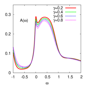
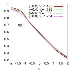
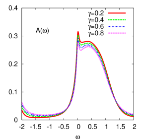
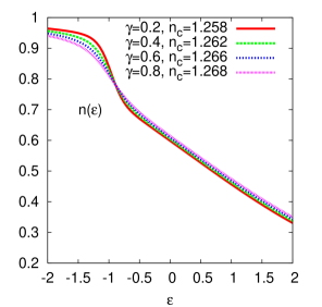
Figure 11: Spectral functions $A(\omega)$ (left panels) and distribution functions $n(\epsilon)$ (right panels) for different couplings $\gamma$ to a heat bath with $\beta=50$. Top panels: $J=1.5$. Bottom panels: $J=2.5$.

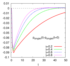
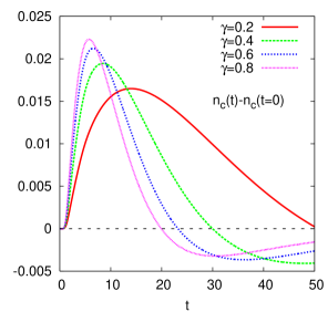
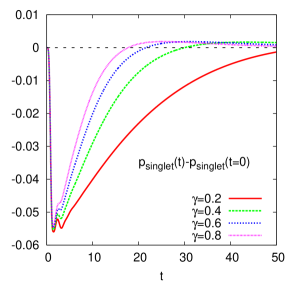
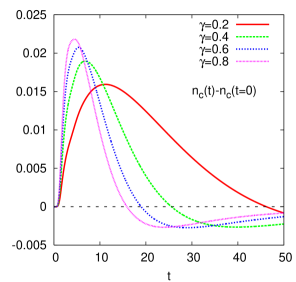
Figure 12: Time-evolution of the probability of the singlet state (left panels) and the density (right panels) for indicated couplings $\gamma$ to the bath with $\beta=50$. The perturbation is a magnetic field pulse of amplitude $h_{x}=0.5$ and duration $t_{\text{max}}=1.5$. A larger coupling $\gamma$ leads to a faster relaxation back to the thermal value. The top panels show data for $J=1.5$ and the bottom panels for $J=2.5$.

In the following we will focus on values of $\gamma$ which are large enough to allow for a fast energy dissipation, but still so small that the equilibrium properties of the system remain qualitatively unchanged with respect to the isolated system. We will therefore first study the effect of the bath (with inverse temperature $\beta=50$) on the spectral function and momentum distribution function in equilibrium. As shown in the left panels of Fig. 11, a stronger coupling $\gamma$ reduces the peak near $\omega=0$ in the spectral function, which is associated with the heavy quasi-particle band. Spectral weight is added to the gap region. As a result, the step-like feature in the distribution function $n(\epsilon)$ (near $\epsilon=-1$) gets smeared out and for $J=1.5$, $n_{c}\approx 1.20$ it is hardly evident anymore for $\gamma\gtrsim 0.4$ (right panels). To obtain a more prominent large Fermi surface, but still keep a strong coupling $\gamma$ to the environment, we also consider data for $J=2.5$ and $n_{c}\approx 1.26$ (bottom panels). While the average density is affected by the coupling to the bath, this effect is comparatively small: $n_{c}$ increases only by about one percent for a coupling strength $\gamma=0.8$.

The time evolution of the system after an intense magnetic field pulse with strength $h_{x}=0.5$ and duration $t_{\text{max}}=1.5$ is plotted in Fig. 12. The left panels show the weight of the average occupation of the singlet state, and the right panels show the density. The larger the coupling $\gamma$, the faster these observables relax back to approximately the thermal value: If one defines a relaxation timescale $\tau_{0.002}$ for this initial fast relaxation as the time by which $p_{\text{singlet}}$ reaches its thermalized value up to within $\pm 0.002$, one finds that these relaxation times $\tau_{0.002}$ scale approximately linearly with $1/\gamma$ ( $J=1.5$: $\tau_{0.002}=62$, $36$, $26.5$, $22$ for $\gamma=0.2,0.4,0.6,0.8$, respectively; $J=2.5$: $\tau_{0.002}=48$, $26$, $19$, $15.5$ for $\gamma=0.2,0.4,0.6,0.8$ ).

The fast initial relaxation leads to an overshooting of the singlet occupation and density, and it is followed by a slower convergence to the true steady state. The fast dynamics can be identified with the formation of the Kondo gap (more precisely, a pseudo-gap), while the slow relaxation is related to the appearance of the heavy quasi-particle band. To illustrate this fact, we plot in Fig. 13 the time-dependent spectral function [Eq. (5)] for several times after the pulse. footnote01 For $J=1.5$, $\gamma=0.6$ (top panels), first indications of a feature near $\omega=0$ appear around $t=20$ (which is the time needed for $p_{\text{singlet}}$ to relax back to roughly the thermal value), with a well-formed peak and a fully established gap around $t=30$. However, the comparison with the equilibrium spectral function (black curve) shows that the amplitude of this peak is enhanced compared to the equilibrium peak (Fig. 13, middle panels), and the recovery of the latter takes much longer (the thermal curve is not reached for $t\approx 40$, which is the largest time for which we can compute well-resolved spectra). The observed long times needed to restore the heavy quasi-particle band are consistent with the relaxation times $\tau\approx 50$ measured for weak perturbations of the FL (Fig. 8).footnote02 Together with the corresponding feature at the lower gap edge, the formation of this coherent quasiparticle peak constitutes the bottleneck in the relaxation process.

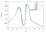
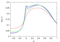
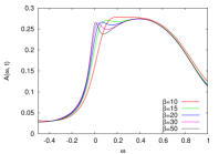
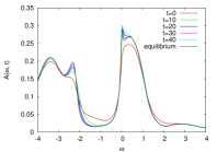
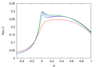
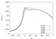
Figure 13: Time-evolution of the spectral function $A(\omega,t)$ for $\gamma=0.6$, $J=1.5$ (top panel) and $J=2.5$ (bottom panel). The left panels show the time-evolution on a wide frequency scale and the middle panels a zoom of the quasi-particle peak. For comparison, the right hand panels illustrate the evolution of the equilibrium spectral function with temperature.

The shape of the peak in $A(\omega,t)$ near $\omega=0$ indicates that the system does not approach the heavy Fermi liquid through a sequence of equilibrium states with decreasing temperature. Instead, it first establishes some kind of fairly stable non-thermal “precursor” state, which slowly evolves into the heavy Fermi liquid. In fact, comparison of the time-dependent spectra to equilibrium spectra at higher temperatures (Fig. 13, right panels) shows that for increased temperature the quasi-particle peak would be broadened (and thus its maximum is shifted towards higher frequency), while in the time-dependent spectra, the location of the peak stays almost constant for large times. The larger amplitude of the peak in the precursor state can also not be explained with the small, transient change in doping - this would rather suggest a less prominent quasi-particle peak, since for large times the doping is slightly smaller than in the final state (Fig. 12). To further illustrate the difference between the non-thermal state with enhanced quasi-particle peak and the true FL equilibrium state, we plot in Fig. 14 the time-evolution of the momentum distribution function $n(\epsilon_{k},t)$. The application of the pulse destroys the step-like feature marking the large Fermi surface. The fast relaxation of the singlet occupation and density back to the thermal values is associated with a partial recovery of the step in $n(\epsilon_{k},t)$, but it is clear from Fig. 14 that after $t=20$ ($\gamma=0.6$) or $t=50$ ($\gamma=0.2$) the distribution function has not yet thermalized. The thermal distribution function with its well-defined step feature is only recovered once the heavy quasi-particle band has been fully reconstructed.

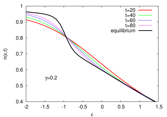
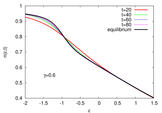
Figure 14: $J=2.5$. Time-evolution of the momentum distribution function for couplings $\gamma=0.2$ (top) and $\gamma=0.6$ (bottom) to the bath with $\beta=50$.

IV Summary and Conclusion

We studied the relaxation dynamics of the Kondo lattice model (restricted to paramagnetic phases) using the nonequilibrium dynamical mean field formalism and an NCA impurity solver which exactly treats an eight-dimensional local problem consisting of a spin and its associated conduction electron orbital. This approach is well-suited to describe the formation of local singlets, which are favored by antiferromagnetic $J$. Comparison to data obtained with the numerically exact CT-HYB solver showed that the NCA approximation yields qualitatively correct results in equilibrium over a wide doping and temperature regime. In particular, it captures the crossover from a local moment regime into the heavy Fermi liquid regime as temperature is lowered in the doped system, with two crossover scales $T_{K}$ (opening of a pseudo-gap in the conduction electron spectral function) and $T^{*}$ (shift in the real part of the conduction electron self-energy and formation of a large Fermi surface).

We determined the relaxation times in these various phases and crossover regimes by applying a weak magnetic field pulse which perturbs the local singlets. While these numbers are related to equilibrium properties of the system, they may still be nontrivial to extract from a conventional imaginary-time equilibrium calculation. In the doped system, the relaxation time grows with decreasing temperature, approximately proportional to the real part of the conduction electron self-energy. The slow relaxation in the heavy Fermi liquid phase is thus clearly associated with the existence of coherent heavy quasi-particles, and not, for example, with the presence of a pseudo-gap in the conduction electron spectral function. The relaxation time was also found to depend strongly on doping, with long relaxation times in the weakly doped heavy Fermi liquid regime. In contrast to the Hubbard model, the relaxation times in the (Kondo) insulating state are substantially shorter than in the weakly doped regime, at least for $J$ comparable to the hopping.

To study the relaxation dynamics of strongly excited systems we considered quenches of the Kondo coupling and strong magnetic field pulses. Such perturbations lead to a considerable heating and it is thus easy to simulate the destruction of the low-temperature heavy-Fermi liquid state. By computing the time-dependent momentum distribution function for quenches from intermediate to small $J$, we could demonstrate the destruction of the step feature associated with the large Fermi surface within a time of a few inverse hopping and the shift from a large to a small Fermi surface on a slower time scale (the relaxation time of the thermal state).

In order to demonstrate the formation of the large Fermi surface upon cooling, we simulated the time-evolution after a strong magnetic field pulse in the presence of a thermal particle reservoir, which removed the excess energy injected by the pulse. While a strong coupling to the heat-bath leads to a faster relaxation, it also smears out the heavy quasi-particle band. Nevertheless, for large enough Kondo coupling and large enough doping, one can have a well-defined large Fermi surface at low temperatures and fast relaxation. By computing the time-dependent momentum distribution functions and spectral functions we could show that the relaxation back to the thermal state happens in two stages: after a fast initial relaxation (whose time-scale depends on the strength of the coupling to the bath), a precursor state to the heavy Fermi liquid is formed, as evidenced by the appearance of a peak near the Fermi energy in the conduction electron spectral function, and a partially reconstructed step feature in the momentum distribution function. This fast relaxation is followed by a slower dynamics (presumably on time scales controlled by the long relaxation time in the heavy Fermi liquid), which leads to the thermalization of the narrow quasi-particle band also in the close vicinity of the Fermi energy.

The existence and the nature of the precursor state should certainly be corroborated and further studied in future investigations. For example, it would be desirable to systematically look at those states at a slightly weaker coupling to the environment in order to reduce the influence of the bath on the FL properties, in particular the quasi-particle weight and FL relaxation rate. However, smaller dissipation requires larger simulation times, which are not accessible within our current (single-processor) implementation of the NCA equations. Furthermore, it would be desirable, although computationally quite expensive, to check the influence of the NCA approximation through a comparison to real-time results from higher order implementations of the self-consistent strong-coupling formalism.

The calculations in this paper were limited to the paramagnetic phases of the antiferromagnetic Kondo lattice model. Many heavy electron materials however are close to a magnetic instability. It would be interesting to extend our study to symmetry broken phases in order to enable an interplay between electronic and magnetic excitations.

Appendix A DMFT self-consistency with bath

In this Appendix we briefly explain how a thermal fermionic bath can be incorporated into the DMFT equations for a semielliptic density of states.

The local $c$-electron Green function of the impurity model, $G_{c}(t,t^{\prime})=-i\text{Tr}[T_{\mathcal{C}}e^{\mathcal{S}}c(t)c^{\dagger}(t^{\prime})]/\text{Tr}[T_{\mathcal{C}}e^{\mathcal{S}}]$ implicitly defines the self-energy $\Sigma$ via the impurity Dyson equation

$$G_{c}(t,t^{\prime})=[i\partial_{t}+\mu-\Delta(t,t^{\prime})-\Sigma(t,t^{\prime})]^{-1}.$$ (9)

Here and in the following, time arguments are on the Keldysh contour $\mathcal{C}$, and $T_{\mathcal{C}}$ is the time-ordering operator on $\mathcal{C}$. We use the notation for Keldysh equations detailed in Ref. Eckstein10quench, . Momentum-dependent lattice Green functions $G_{\boldsymbol{k}}(t,t^{\prime})=-i\langle T_{\mathcal{C}}c_{\boldsymbol{k}}(t)c_{\boldsymbol{k}}^{\dagger}(t^{\prime})\rangle$ are then obtained from the lattice Dyson equation

$$G_{\boldsymbol{k}}(t,t^{\prime})=[i\partial_{t}+\mu-\epsilon_{\boldsymbol{k}}-\Sigma(t,t^{\prime})]^{-1},$$ (10)

where $\epsilon_{\boldsymbol{k}}$ is the noninteracting dispersion. From these functions the time-dependent momentum distribution can be obtained,

$$n(\epsilon_{\boldsymbol{k}},t)=-iG_{\boldsymbol{k}}^{<}(t,t).$$ (11)

For a lattice whose noninteracting density of states is semi-elliptical with bandwidth $4v$, the local (momentum averaged) lattice Greenfunction can be shown to satisfy the self-consistent equation

$$G(t,t^{\prime}) \equiv\sum_{\boldsymbol{k}}G_{\boldsymbol{k}}(t,t^{\prime})$$ (12)

$$=[i\partial_{t}+\mu-v^{2}G(t,t^{\prime})-\Sigma(t,t^{\prime})]^{-1}.$$ (13)

Note that the second equality does not depend on the form of the self-energy, but only on the distribution of the band-energies $\epsilon_{\boldsymbol{k}}$.SFB Comparison with the impurity Dyson equation (9) then yields the standard DMFT self-consistency condition, Eq. (4).

If an additional fermionic reservoir is coupled to the lattice at every site, one has to modify the lattice Dyson equation (10) by adding the hybridization function $\Delta_{\beta}(t,t^{\prime})$ to the free dispersion,

$$G_{\boldsymbol{k}}(t,t^{\prime})=[i\partial_{t}+\mu-\epsilon_{\boldsymbol{k}}-\Delta_{\beta}(t,t^{\prime})-\Sigma(t,t^{\prime})]^{-1}.$$ (14)

Hence the closed form equation for the momentum averaged Green function becomes

$$G(t,t^{\prime})=[i\partial_{t}+\mu-v^{2}G(t,t^{\prime})-\Delta_{\beta}(t,t^{\prime})-\Sigma(t,t^{\prime})]^{-1},$$ (15)

and, by comparison with Eq. (9), we obtain the DMFT self-consistency with fermionic bath,

$$\Delta(t,t^{\prime})=v^{2}G(t,t^{\prime})+\Delta_{\beta}(t,t^{\prime}).$$ (16)

References

- (1) Y. Kuramoto and Y. Kitaoka, Dynamics of Heavy Electrons (Oxford University Press, New York, 2000).
- (2) P. Coleman, in Handbook of Magnetism and Advanced Magnetic (J. Wiley and Sons, 2007).
- (3) S. Doniach, Physica B 91, 231 (1977).
- (4) P. Werner and A. J. Millis, Phys. Rev. B 74, 155107 (2006).
- (5) M. Oshikawa, Phys. Rev. Lett. 84, 3370 (2000).
- (6) J. Otsuki, H. Kusunose, and Y. Kuramoto, Phys. Rev. Lett. 102, 017202 (2009).
- (7) J. Otsuki, H. Kusunose, and Y. Kuramoto, J. Phys. Soc. Jpn. 78, 034719 (2009).
- (8) A. Georges, G. Kotliar, W. Krauth and M. J. Rozenberg, Rev. Mod. Phys. 68, 13 (1996).
- (9) M. Metzner and D. Vollhard, Phys. Rev. Lett. 62, 324(1989).
- (10) P. Schmidt and H. Monien, arXiv:cond-mat/0202046 (unpublished).
- (11) J. K. Freericks, V. M. Turkowski, and V. Zlatić, Phys. Rev. Lett. 97, 266408 (2006).
- (12) R. Bulla, T. A. Costi, and T. Pruschke, Rev. Mod. Phys. 80, 395 (2008).
- (13) E. Gull, A. J. Millis, A. N. Rubtsov, A. I. Lichtenstein, M. Troyer and P. Werner, Rev. Mod. Phys. 83, 349 (2011).
- (14) J. Otsuki, H. Kusunose, P. Werner, and Y. Kuramoto, J. Phys. Soc. Jpn. 76, 114707 (2007).
- (15) P. Werner, T. Oka, and A. J. Millis, Phys. Rev. B 79, 035320 (2009).
- (16) P. Werner, T. Oka, M. Eckstein, and A. J. Millis, Phys. Rev. B 81, 035108 (2010).
- (17) M. Eckstein and P. Werner, Phys. Rev. B 82, 115115 (2010).
- (18) Th. Pruschke, B. Steininger, J. Keller, Physica B 206 207 154 (1995).
- (19) If a smaller local Hilbert space is used, this physics requires the summation of higher-order diagrams beyond the NCA.
- (20) M. Eckstein, M. Kollar and P. Werner, Phys. Rev. B 81, 115131 (2010).
- (21) J. K. Freericks, H. R. Krishnamurthy, and Th. Pruschke, Phys. Rev. Lett. 102, 136401 (2009); M. Eckstein and M. Kollar, Phys. Rev. B 78, 245113 (2008).
- (22) E. Gull, D. Reichmann and A. J. Millis, Phys. Rev. B 84, 085134 (2011).
- (23) S. Burdin, A. Georges, and D. R. Grempel, Phys. Rev. Lett. 85, 1048 (2000).
- (24) M. Eckstein and P. Werner, Phys. Rev. B 84, 035122 (2011).
- (25) N. Tsuji, T. Oka and H. Aoki, Phys. Rev. Lett. 103, 047403 (2009).
- (26) A. Amaricci, C. Weber, M. Capone and G. Kotliar, arXiv:1106.3483.
- (27) To avoid oscillations due to a cutoff in the Fourier integral in Eq. (5), we have extrapolated to large times using an exponential function. This is possible, because in the model with bath, the oscillations in are damped rather quickly.
- (28) In the presence of the bath the FL relaxation rate is somewhat reduced.
- (29) M. Eckstein, A. Hackl, S. Kehrein, M. Kollar, M. Moeckel, P. Werner and F. A. Wolf, Eur. Phys. J. Special Topics 180, 217 (2010).