Rare B decays in the $\cal F$-$SU(5)$ Model

Abstract

In the testable Flipped $SU(5)\times U(1)_{X}$ model with TeV-scale vector-like particles from F-theory model building dubbed as the $\cal F$-$SU(5)$ model, we study the vector-like quark contributions to B physics processes, including the quark mass spectra, Feynman rules, new operators and Wilson coefficients, etc. We focus on the implications of the vector-like quark mass scale on B physics. We find that there exists the $\bar{s}bZ$ interaction at tree level, and the Yukawa interactions are changed. Interestingly, different from many previous models, the effects of vector-like quarks on rare B decays such as $B\to X_{s}\gamma$ and $B\to X_{s}\ell^{+}\ell^{-}$ do not decouple in some viable parameter space, especially when the vector-like quark masses are comparable to the charged Higgs boson mass. Under the constraints from $B\to X_{s}\gamma$ and $\ B\to X_{s}\ell^{+}\ell^{-}$, the latest measurement for $B_{s}\to\mu^{+}\mu^{-}$ can be explained naturally, and the branching ratio of $B_{s}\to\ell^{+}\ell^{-}\gamma$ can be up to $(4\sim 5)\times 10^{-8}$. The non-decouling effects are much more predictable and thus the $\cal F$-$SU(5)$ model may be tested in the near future experiments.

I Introduction

Supersymmetry provides a natural solution to the gauge hierarchy problem in the Standard Model (SM). In the supersymmetric SM (SSM) with R-parity under which the SM particles are even while the supersymmetric particles (sparticles) are odd, the $SU(3)_{C}\times SU(2)_{L}\times U(1)_{Y}$ gauge couplings can be unified around $2\times 10^{16}$ GeV Langacker:1991an , the lightest supersymmetric particle (LSP) such as the neutralino can be a cold dark matter candidate Ellis:1983ew ; Goldberg:1983nd , and the electroweak (EW) precision constraints can be evaded, etc. Especially, the gauge coupling unification strongly suggests Grand Unified Theories (GUTs). However, in the supersymmetric $SU(5)$ models, there exist the doublet-triplet splitting problem and dimension-five proton decay problem. Interestingly, these problems can be solved elegantly in the Flipped $SU(5)\times U(1)_{X}$ models smbarr ; dimitri ; AEHN-0 via missing partner mechanism AEHN-0 . On the other hand, string theory is the most promising candidate for quantum gravity, and it can unify all the fundamental interactions in the Nature. However, the string scale is at least one-order larger than the conventional GUT scale.

To solve the little hierarchy problem between the traditional GUT scale and string scale, two of us (TL and DVN) with Jing Jiang have proposed the testable Flipped $SU(5)\times U(1)_{X}$ models, where the TeV-scale vector-like particles are introduced Jiang:2006hf . Such kind of models can be constructed from the free fermionic string constructions at the Kac-Moody level one Antoniadis:1988tt ; Lopez:1992kg and locally from the F-theory model building Beasley:2008dc ; Jiang:2009zza , and is dubbed as ${\cal F}$-$SU(5)$ Jiang:2009zza . In particular, these models are very interesting from the phenomenological point of view Jiang:2009zza : the vector-like particles can be observed at the Large Hadron Collider (LHC), proton decay is within the reach of the future Hyper-Kamiokande Nakamura:2003hk and Deep Underground Science and Engineering Laboratory (DUSEL) DUSEL experiments Li:2009fq ; Li:2010dp , the hybrid inflation can be naturally realized, the correct cosmic primodial density fluctuations can be generated Kyae:2005nv , and the lightest CP-even Higgs boson mass can be lifted Huo:2011zt ; Li:2011ab . With no-scale boundary conditions at $SU(5)\times U(1)_{X}$ unification scale Cremmer:1983bf , two of us (TL and DVN) with James Maxin and Joel Walker have described an extraordinarily constrained “golden point” Li:2010ws and “golden strip” Li:2010mi that satisfied all the latest experimental constraints and has an imminently observable proton decay rate Li:2009fq . For a review of the recent progresses, see Ref. Li:2012uj .

Interestingly, the vector-like quarks in the $\cal F$-$SU(5)$ model predict rich phenomenology on low energy processes. If the model is treated seriously, constraints from electroweak parameters such as $U,\ S,T$ and $R_{b},\ R_{c}$ and B processes should be taken into account. We also would like to point out that the $\cal F$-$SU(5)$ model has no Landau pole problem and then is very different from the other simple SM extensions in quark sector (also see the next Section) BNPfourth , and the $3\times 3$ SM-like quark mixing matrix is now replaced by a $5\times 5$ one and then is no longer unitary, and there exists the tree-level $\bar{s}bZ$ interaction, which will play an important, even dominant, role in some parameter space for rare B decays.

Thanks to the efforts of the B factories and LHC, the exploration of quark-flavor mixing is now entering a new interesting era. It is well known that the rare B decays induced by the flavor changing neutral current (FCNC) only occur at loop level in the SM and then are sensitive to new physics. Thus, the rare radiative, leptonic and semi-leptonic B meson decays are valuable in testing the SM at loop level and probe new physics. On the theoretical side, the rare B inclusive radiative decays $B\to X_{s}\gamma$ and $B\to X_{s}\ell^{+}\ell^{-}(\ell=e,\mu)$ as well as the exclusive decays $B_{s}\to\mu^{+}\mu^{-}$ and $B_{s}\to\ell^{+}\ell^{-}\gamma$ have been studied extensively at the leading logarithm order (LO) BLOSM and high order in the SM BHOSM and various new physics models BNPfourth ; BNPMSSM ; BNP2HDM . On the experimental side, $B\to X_{s}\gamma$ and $B\to X_{s}\ell^{+}\ell^{-}(\ell=e,\mu)$ have been measured and the latest upper bound on $B_{s}\to\mu^{+}\mu^{-}$ is achieved Bmeasured . By comparing the predictions with experimental measurements, we will present some constraints on the parameter space in the $\cal F$-$SU(5)$ model.

The first task of this work will be deriving the quark mass spectra and Feynman rules. We stress that the Feynman rules which not be presented in previous studies are used not only in B physics but also in research of all low energy processes. B physics constraints on the model is the second task of this work, we will concentrate our attention on the vector-like quark contributions to B physics, in particular, the contributions from the new operators induced by tree-level FCNC. We will show that the $\bar{s}bZ$ interaction can be generated at tree level, and the Yukawa interactions are changed, new operators $O_{9}^{\prime}$ and $O_{10}^{\prime}$ in effective Hamiltonian should be introduced. We will demonstrate that different from many previous models, the effects of vector-like quarks on rare B decays such as $B\to X_{s}\gamma$ and $B\to X_{s}\ell^{+}\ell^{-}$ do not decouple in some allowed parameter space, especially when the vector-like quark masses are comparable to the charged Higgs boson mass. Within the constraints from $B\to X_{s}\gamma$ and $\ B\to X_{s}\ell^{+}\ell^{-}$, and the latest measurement for $B_{s}\to\mu^{+}\mu^{-}$ will be explained naturally, and the branching ratio of $B_{s}\to\ell^{+}\ell^{-}\gamma$ can be up to $(4\sim 5)\times 10^{-8}$. Because the non-decouling effects are very predictable, the $\cal F$-$SU(5)$ model may be tested in the near future experiments.

This paper is organized as follows. We present a brief description for the TeV-scale $\cal F$-$SU(5)$ model and derive all the Feynman rules for our calculations in Section II. We discuss the implications of vector-like quarks on B physics in Section III. Our numerical results are presented in Section IV, and Section V is the summary.

II The $\cal F$-$SU(5)$ Model around the TeV Scale

To achieve the string-scale gauge coupling unification in the $\cal F$-$SU(5)$ model, we introduce the vector-like particles which from complete Flipped $SU(5)\times U(1)_{X}$ multiplets. The quantum numbers for these additional vector-like particles under the $SU(5)\times U(1)_{X}$ gauge symmetry are Jiang:2006hf

$$XF={\mathbf{(10,1)}}~{},~{}{\overline{YF}}={\mathbf{({\overline{10}},-1)}}~{},~{}$$

$$Xf={\mathbf{(5,3)}}~{},~{}{\overline{Yf}}={\mathbf{({\overline{5}},-3)}}~{},~{}$$

$$Xl={\mathbf{(1,-5)}}~{},~{}{\overline{Yl}}={\mathbf{(1,5)}}~{}.~{}$$ (1)

To avoid the confusion in the following discussions, we change the convention in Ref. Jiang:2006hf a little bit. It is obvious that $XF$, ${\overline{YF}}$, $Xf$, ${\overline{Yf}}$, $Xl$, and ${\overline{Yl}}$ are standard vector-like particles with contents as follows

$$XF=(XQ,XD^{c},XN^{c})~{},~{}{\overline{YF}}=(YQ^{c},YD,YN)~{},~{}$$

$$Xf=(XU,XL^{c})~{},~{}{\overline{Yf}}=(YU^{c},YL)~{},~{}$$

$$Xl=XE~{},~{}{\overline{Yl}}=YE^{c}~{}.~{}$$ (2)

Under the $SU(3)_{C}\times SU(2)_{L}\times U(1)_{Y}$ gauge symmetry, the quantum numbers for the extra vector-like particles are

$$XQ={\mathbf{(3,2,{1\over 6})}}~{},~{}YQ^{c}={\mathbf{({\bar{3}},2,-{1\over 6})}}~{},~{}$$

$$XU={\mathbf{({3},1,{2\over 3})}}~{},~{}YU^{c}={\mathbf{({\bar{3}},1,-{2\over 3})}}~{},~{}$$

$$XD={\mathbf{({3},1,-{1\over 3})}}~{},~{}YD^{c}={\mathbf{({\bar{3}},1,{1\over 3})}}~{},~{}$$

$$XL={\mathbf{({1},2,-{1\over 2})}}~{},~{}YL^{c}={\mathbf{(1,2,{1\over 2})}}~{},~{}$$

$$XE={\mathbf{({1},1,{-1})}}~{},~{}YE^{c}={\mathbf{({1},1,{1})}}~{},~{}$$

$$XN={\mathbf{({1},1,{0})}}~{},~{}YN^{c}={\mathbf{({1},1,{0})}}.$$ (3)

At the GUT scale the superpotential is given by

$$W_{GUT} = Y_{ij}^{D}F_{i}F_{j}h+Y_{ij}^{U\nu}F_{i}\bar{f_{j}}\bar{h}+Y_{ij}^{E}\bar{l_{i}}\bar{f_{j}}h+\mu h\bar{h}+Y_{kj}^{N}\phi_{k}\bar{H}F_{j}$$ (4)

$$+ Y^{\prime}{}_{j}^{D}XFF_{j}h+Y^{\prime}{}_{j}^{U\nu}XF\bar{f}_{j}\bar{h}+Y"{}_{i}^{U\nu}F_{i}\overline{Xf}\bar{h}+Y^{\prime}{}_{j}^{E}\overline{Xl}\bar{f}_{j}h$$

$$+ Y"{}_{j}^{E}\bar{l}_{j}\overline{Xf}h+Y^{\prime}{}_{k}^{N}\phi_{k}\bar{H}XF+Y^{2D}XFXFh+Y^{\prime 2D}\overline{YF}\overline{YF}\bar{h}$$

$$+ Y^{2U\nu}XF\overline{Xf}\bar{h}+Y^{\prime 2U\nu}\overline{YF}Yfh+Y{}^{2E}\overline{Xl}\overline{Xf}h+Y^{\prime 2E}YlYf\bar{h}$$

$$+ M_{j}^{1}F_{j}\overline{YF}+M_{j}^{2}\bar{f}_{j}Yf+M_{j}^{3}\bar{l}_{j}Yl$$

$$+ M^{4}XF\overline{YF}+M^{5}\overline{Xf}Yf+M^{6}\overline{Xl}Yl~{},$$

where $i$ is the generation indices. The first line is the SSM superpotential, the second line is the Yukawa mixing terms between the SM fermions and vector-like particles, the third and fourth lines are the SM-like superpotential for vector-like multiplets, and the fifth and sixth lines are bilinear mass terms. After the $SU(5)\times U(1)_{X}$ gauge symmetry breaking down to the SM gauge symmetry, we obtain the superpotential as follows

$$W_{EW} = (Y_{ij}^{D}-Y_{ji}^{D})(D^{c})_{i}Q_{j}\cdot H_{d}+Y_{ij}^{U\nu}U_{j}^{c}Q_{i}\cdot H_{u}-Y_{ij}^{U\nu}N_{i}^{c}L_{j}\cdot H_{u}$$ (5)

$$- Y_{ij}^{E}E_{i}^{c}L\cdot H_{d}-Y_{j}^{{}^{\prime}D}(XD^{c}Q_{j}\cdot H_{d}+D_{j}^{c}XQ\cdot H_{d})+Y_{{}^{\prime}j}^{U\nu}U_{j}^{c}XQ\cdot H_{u}$$

$$- Y_{j}^{{}^{\prime}U\nu}XN^{c}L\cdot H_{u}+Y_{i}^{"U\nu}XU^{c}Q\cdot H_{u}-Y_{i}^{"U\nu}N_{i}^{c}XL\cdot H_{u}-Y_{j}^{{}^{\prime}E}XE^{c}L\cdot H_{d}$$

$$- Y_{j}^{"E}E_{j}^{c}XL\cdot H_{d}-2Y^{2D}XD^{c}XQ\cdot H_{d}-2Y^{{}^{\prime}2D}YDYQ^{c}\cdot H_{u}$$

$$+ Y^{2U\nu}XU^{c}XQ\cdot H_{u}-Y^{2U\nu}XN^{c}XL\cdot H_{u}-Y^{{}^{\prime}2U\nu}YUYQ^{c}\cdot H_{d}$$

$$+ Y^{{}^{\prime}2U\nu}YNYL^{c}\cdot H_{d}-Y^{2E}XE^{c}XL\cdot H_{d}-Y^{{}^{\prime}2E}YEYL^{c}\cdot H_{u}$$

$$- 2M_{j}^{1}\left[D_{j}^{c}YD+Q\cdot YQ^{c}+N_{j}^{c}YN\right]+M_{j}^{2}\left[U^{c}YU+L\cdot YL^{c}\right]+M_{j}^{3}E_{j}^{c}YE$$

$$- 2M^{4}\left[XD^{c}YD+XQ\cdot YQ^{c}+XN^{c}YN\right]+M^{5}\left[XU^{c}YU+XL\cdot YL^{c}\right]$$

$$+ M^{6}XE^{c}YE~{}.~{}\,$$

At low energy, the sparticles decouple rapidly when $M_{S}$ increases. Note that the LHC already put strong constraints on squark masses around 1500 GeV, we will concentrate on the contributions from new vector-like quark multiplets $XU,~{}YU^{c},~{}XD,~{}{\rm and}~{}YD^{c}$ for simplicity. At first glance these multiplets seem to be similar to the fourth and fifth generation quarks, but indeed $(XU,~{}YU^{c})$ and $(XD,~{}YD^{c})$ are vector-like. This makes them very different from the fourth and fifth generation quarks. The down-type quark mass matrix is

$$M_{D}= \left(\begin{array}[]{ccccc}(Y_{11}^{D}+Y_{11}^{D})v_{d}&(Y_{12}^{D}+Y_{21}^{D})v_{d}&(Y_{13}^{D}+Y_{31}^{D})v_{d}&Y^{\prime}{}_{1}^{D}v_{d}&-2M_{1}^{1}\\ (Y_{21}^{D}+Y_{12}^{D})v_{d}&(Y_{22}^{D}+Y_{22}^{D})v_{d}&(Y_{23}^{D}+Y_{32}^{D})v_{d}&Y^{\prime}{}_{2}^{D}v_{d}&-2M_{2}^{1}\\ (Y_{31}^{D}+Y_{13}^{D})v_{d}&(Y_{32}^{D}+Y_{23}^{D})v_{d}&(Y_{33}^{D}+Y_{33}^{D})v_{d}&Y^{\prime}{}_{3}^{D}v_{d}&-2M_{3}^{1}\\ Y^{\prime}{}_{1}^{D}v_{d}&Y^{\prime}{}_{2}^{D}v_{d}&Y^{\prime}{}_{3}^{D}v_{d}&2Y^{2D}v_{d}&-2M^{4}\\ 2M_{1}^{1}&2M_{2}^{1}&2M_{3}^{1}&2M^{4}&-2Y^{\prime 2D}v_{u}\end{array}\right)~{},~{}$$ (11)

and the up-type quark matrix is

$$M_{U}=\left(\begin{array}[]{ccccc}Y_{11}^{U\nu}v_{u}&Y_{21}^{U\nu}v_{u}&Y_{31}^{U\nu}v_{u}&Y^{\prime}{}_{1}^{U\nu}v_{u}&M_{1}^{2}\\ Y_{12}^{U\nu}v_{u}&Y_{22}^{U\nu}v_{u}&Y_{32}^{U\nu}v_{u}&Y^{\prime}{}_{2}^{U\nu}v_{u}&M_{2}^{2}\\ Y_{13}^{U\nu}v_{u}&Y_{23}^{U\nu}v_{u}&Y_{33}^{U\nu}v_{u}&Y^{\prime}{}_{3}^{U\nu}v_{u}&M_{3}^{2}\\ Y"{}_{1}^{U\nu}v_{u}&Y"{}_{2}^{U\nu}v_{u}&Y"{}_{3}^{U\nu}v_{u}&Y^{2U\nu}v_{u}&M^{5}\\ -2M_{1}^{1}&-2M_{2}^{1}&-2M_{3}^{1}&-2M^{4}&Y^{\prime 2U\nu}v_{d}\end{array}\right)~{},~{}$$ (17)

where $v_{u}$ and $v_{d}$ are the vacuum expectation values (VEVs) for $H_{u}$ and $H_{d}$. These two matrixes can be diagonalized by unitary matrices $U$ and $V$,

$$V_{d}^{\dagger}M_{D}U_{d}={\rm diag.}[m_{d},m_{s},m_{b},m_{d_{x}},m_{d_{y}}],$$

$$V_{u}^{\dagger}M_{U}U_{u}={\rm diag.}[m_{u},m_{c},m_{t},m_{u_{x}},m_{u_{y}}].$$ (18)

Thus, the quark mixings are described by a matrix $V=U_{u}^{\dagger}U_{d}$. From Eqs. (11) and (17), we can see that the mass matrices of the down-type quarks and up-type quarks are related to each other, implying that the Yukawa couplings are different from those in the SM. In the Feynman gauge the Feynman rules for charged $W$ boson, Goldstone boson, and charged Higgs boson with quarks $\overline{u_{l}}d_{j}\chi^{+}(\chi=W,~{}G,~{}h)$ and for $Z$ boson $\overline{d_{j}}d_{l}Z$ needed in our calculations are given as follows

$$i\frac{g}{\sqrt{2}}\gamma^{\mu}\left[g^{\chi}_{L}(l,j)P_{L}+g^{\chi}_{R}(l,j)P_{R}\right],~{}~{}(\chi=W,~{}Z)~{},$$ (19)

$$i\frac{g}{\sqrt{2}}\left[g^{\chi}_{L}(l,j)P_{L}+g^{\chi}_{R}(l,j)P_{R}\right],~{}~{}(\chi=G,~{}h)~{},$$ (20)

where

$$g^{W}_{L}(i,j) = \sum_{m=1}^{4}U_{u}^{*mi}U_{d}^{m,j},\ \ \ g^{W}_{R}(i,j)=V_{u}^{*5i}V_{d}^{5j},$$ (21)

$$g^{Z}_{L}(i,j) = -\frac{1}{\sqrt{2}\cos\theta_{W}}\left[\left(1-\frac{2}{3}\sin^{2}\theta_{W}\right)\delta^{ij}-U_{d}^{*5i}U_{d}^{5j}\right],$$

$$g^{Z}_{R}(i,j) = -\frac{1}{\sqrt{2}\cos\theta_{W}}\left[-\frac{2}{3}\sin^{2}\theta_{W}\delta^{ij}+V_{d}^{*5i}V_{d}^{5j}\right],$$ (22)

$$g^{G}_{L}(i,j) = \left(\sum_{k,m=1}^{4}Y^{U\nu}_{km}V_{u}^{*ki}U_{d}^{mj}+2Y^{\prime 2D}V_{u}^{*5i}U_{d}^{5j}\right)\frac{v_{u}}{m_{W}},$$

$$g^{G}_{R}(i,j) = -\left(\sum_{k,m=1}^{4}(Y^{D}_{mk}+Y^{D}_{km})V_{d}^{*kj}U_{u}^{mi}-2Y^{\prime U\nu}V_{d}^{*5j}U_{d}^{5i}\right)\frac{v_{d}}{m_{W}},$$ (23)

$$g^{h}_{L}(i,j) = \left(\sum_{k,m=1}^{4}Y^{U\nu}_{km}V_{u}^{*ki}U_{d}^{mj}+2Y^{\prime 2D}V_{u}^{*5i}U_{d}^{5j}\right)\frac{v_{d}}{m_{W}},$$

$$g^{h}_{R}(i,j) = \left(\sum_{k,m=1}^{4}(Y^{D}_{mk}+Y^{D}_{km})V_{d}^{*kj}U_{u}^{mi}-2Y^{\prime U\nu}V_{d}^{*5j}U_{d}^{5i}\right)\frac{v_{u}}{m_{W}}.$$ (24)

Because the vector-like particles do not change $U(1)_{EM}$ interaction, the interactions of photon and quarks are still the same as those in the SM. From the above mass matrices we can see that the TeV-scale $\cal F$-$SU(5)$ model has two points for rich physics to be explored:

• Since the quark mass matrices are not the same as two Higgs doublet model (2HDM) BNP2HDM or the Minimal Supersymmetric Standard Model (MSSM) BNPMSSM , the loop-level FCNC will be changed by the Yukawa interactions, and then may change the prediction of process $b\to s\gamma$ significantly.

• The last terms in Eqs.(21)-(24), which we call the “tail terms”, will cause the tree-level FCNC processes induced by $b\to s\ell^{+}\ell^{-}$ and then the stringent constraints on the model parameter space will be expected.

III Implications on B physics

Apart from the directly search for the light vector-like quarks at the LHC, another way to test the $\cal F$-$SU(5)$ model is to measure their effects on low energy processes such as rare B decays.

III.1 Effective Hamiltonian

The starting point for rare B decays $B\to X_{s}\gamma$, $B\to X_{s}\ell^{+}\ell^{-}$, $B_{s}\to\ell^{+}\ell^{-}$ and $B_{s}\to\ell^{+}\ell^{-}\gamma$ is the determination of a low-energy effective Hamiltonian obtained by integrating out the heavy degrees of freedom in the theory. For $b\to s$ transition, this can be written as

$${\cal H}_{\rm eff}=-\frac{G_{F}}{\sqrt{2}}V_{ts}^{*}V_{tb}\sum_{i=1}^{10}[C_{i}(\mu)O_{i}(\mu)+C^{{}^{\prime}}_{i}(\mu)O^{{}^{\prime}}_{i}(\mu)]~{},~{}\,$$ (25)

where the effective operators $O_{i}$ are same as those in the SM defined in Ref. BLOSM . The chirality-flipped operators $O^{\prime}_{i}$ are obtained from $O_{i}$ by the replacement $\gamma_{5}\to-\gamma_{5}$ in quark current. It is obvious that $O^{\prime}_{9,10}$ can be got directly from the tail terms in the Feynman rules of the $\cal F$-$SU(5)$ model. A few remarks follow on the operators and Wilson coefficients:

• As mentioned in introduction, the three generation quark mixing matrix is replaced by a $5\times 5$ matrix $U_{u}^{\dagger}U_{d}$ and then is non-unitary. In our analyses we take a reasonable assumption that the deviation from unitary is not large. Otherwise, the tree-level FCNC will modify significantly the low energy processes such as $Z\to b\overline{b}$ and $B_{s}\to\mu^{+}\mu^{-}$.

• Since the Wilson coefficient $C_{2}(m_{W})=-\frac{V_{cb}V_{cs}^{*}}{V_{tb}V_{ts}^{*}}\simeq 1$ is always a good approximation in $\cal F$-$SU(5)$ model, and the coefficients of four quark operators $C_{i}(\mu_{b})\ (i=1,3-6)$ depend actually on the value $C_{2}(m_{W})$, the contributions from the four-quark operator matrix elements to effective coefficient $C_{9}^{eff}(\mu_{b})$ can not be ignored and have the same expressions as the SM.

• The coefficient of operator $O_{2}^{\prime}=(\overline{s}c)_{V+A}(\overline{c}b)_{V-A}$, for example, is proportional to the elements of quark mixing matrix $V^{5j}_{u}$ or $U^{5i}_{d}$ denoted the mixings between the ordinary quarks and vector-like quarks. Thus, it can be reasonably set to be much smaller than $\mathcal{O}(1)$, and the contributions from the four-quark primed operators to $C_{9}^{eff}(\mu_{b})$ and $C_{9}^{{}^{\prime},eff}(\mu_{b})$ can be neglected safely. This means

  $$C_{9,10}^{{}^{\prime},eff}(\mu_{b})=C_{9,10}^{{}^{\prime}}(m_{W})~{},~{}\,$$ (26)

  which receive contributions mainly from the tree-level diagrams, loop diagrams for $b\to s\gamma$, and box diagrams. We also neglect the operator $O_{7}^{\prime}$ contribution.

• For $b\to s\gamma$, the new contributions mainly come from the new type Yukawa interactions, and for $b\to s\ell^{+}\ell^{-}$, the new contributions mainly arise from the new operators $O_{9,10}^{\prime}$.

III.2 Analyses in B Physics Calculations

In the $\cal F$-$SU(5)$ model the contributions to operators $O_{i}\ (i=1-10)$ and $O^{\prime}_{9,10}$ can be encoded by the values of the coefficients $C_{i}$ and $C^{\prime}_{i}$ at the matching scale $m_{W}$. In this Section, we will present the Wilson coefficients at the matching scale and decay widths for some rare B decays. We keep both new physics contributions and the SM results at the LO for consistency.

• The Wilson coefficient $C_{7}$ at the matching scale is

  $$C_{7} = \frac{1}{V_{tb}V_{ts}^{\ast}}\sum_{i=1}^{5}\{A(x_{i})g_{L}^{W\ast}(i,2)g_{L}^{W}(i,3)-B(x_{i})\frac{m_{W}}{m_{b}}g_{L}^{W\ast}(i,2)g_{R}^{G}(i,3)$$ (27)

  $$+ g_{L}^{G\ast}(i,2)[C(x_{i})g_{L}^{G}(i,3)-\frac{m_{u_{i}}}{m_{b}}D(x_{i})g_{R}^{G}(i,3)]$$

  $$+ \frac{x_{i}}{y_{i}}g_{L}^{{h}\ast}(i,2)[C(y_{i})g_{L}^{{h}}(i,3)-\frac{m_{u_{i}}}{m_{b}}D(y_{i})g_{R}^{{h}}(i,3)]\},$$

  where $x_{i}=m_{u_{i}}^{2}/m_{W}^{2}$ and $y_{i}=m_{u_{i}}^{2}/m_{h^{+}}^{2}$. For cross check, using the loop functions given in the appendix and the CKM matrix unitarity condition, one can easily obtain the predication $C_{7}^{SM}(m_{W})=A(x_{t})+B(x_{t})+x_{t}[C(x_{t})+D(x_{t})]$ which is consistent with that in Ref. BLOSM . Furthermore, $C_{7}$ receives a large non-decoupling contribution not only from top quark as in the SM but also from the up-type vector-like quark loops at the electroweak scale. The non-decoupling effects are unique and will be demonstrated in next Section.

  The Wilson coefficient $C_{9}$ at the matching scale is

  $$C_{9} = \frac{P(x_{t})-Q(x_{t})}{\sin^{2}\theta_{W}}+4Q(x_{t})$$ (28)

  $$- \frac{2\pi}{\alpha_{em}}\frac{U_{d}^{*52}U_{d}^{53}}{V_{tb}V_{ts}^{\ast}}(\frac{1}{4}-\sin^{2}\theta_{W})$$

  $$+ \frac{1}{V_{tb}V_{ts}^{\ast}}\left\{\sum_{i=3}^{5}\left[R(x_{i})g_{L}^{W\ast}(i,2)g_{L}^{W}(i,3)+S(x_{i})g_{R}^{G\ast}(i,2)g_{L}^{G}(i,3)\right]\right.$$

  $$+ \sum_{i=1}^{5}\frac{m_{W}}{m_{u_{i}}}T(x_{i})\left[g_{L}^{W\ast}(i,2)g_{L}^{G}(i,3)+g_{R}^{G\ast}(i,2)g_{L}^{W}(i,3)\right]$$

  $$+ \left.\frac{x_{i}}{y_{i}}S(y_{i})g_{R}^{{h}\ast}(i,2)g_{L}^{{h}}(i,3)]\right\}+\frac{4}{9}.$$

  Note the first part related to $P(x_{t})$ and $Q(x_{t})$ from the box diagrams and the effective vertex $b\to sZ^{*}$ at loop level have the same expression as those in the SM, while the second part denotes the interaction at tree level enhanced by a large factor $\frac{2\pi}{\alpha_{em}}$. The last part comes from the effective vertex $b\to s\gamma^{*}$ at loop level for consistency. The contribution from one-loop matrix element of the operator $O_{2}$ is also included as in the SM BLOSM . Moreover, the Wilson coefficients $C_{10}$, $C^{\prime}_{9}$, and $C^{\prime}_{10}$ at the matching scale are

  $$C_{10} = -\frac{P(x_{t})-Q(x_{t})}{\sin^{2}\theta_{W}}+\frac{2\pi}{\alpha_{em}}\frac{1}{4}\frac{U_{d}^{*52}U_{d}^{53}}{V_{tb}V_{ts}^{\ast}}~{},~{}$$ (29)

  $$C_{9}^{{}^{\prime}} = (\frac{1}{4}-\sin^{2}\theta_{W})\frac{2\pi}{\alpha_{em}}\frac{V_{d}^{*52}V_{d}^{53}}{V_{tb}V_{ts}^{\ast}}~{},~{}$$ (30)

  $$C_{10}^{{}^{\prime}} = -\frac{2\pi}{\alpha_{em}}\frac{1}{4}\frac{V_{d}^{*52}V_{d}^{53}}{V_{tb}V_{ts}^{\ast}}~{}.$$ (31)

  The contributions from loop diagrams to $C^{\prime}_{9,10}$ can be neglected safely.

• Branching Ratios
  Considering that the Wilson coefficients do not separate into the SM and new physics parts easily and new operators are introduced, we need to list some explicit expressions for the branching ratios of B decays as follows

  1. $B\to X_{s}\gamma$
     The inclusive $B\to X_{s}\gamma$ rate is the most precise and clean short-distance information that we have, at present, on $\Delta B=1$ FCNCs. The new contributions mainly come from the new type Yukawa interactions to operator $O_{7}$. The calculation of the branching ratio is usually normalized by the process $B\rightarrow X_{c}e\overline{\nu_{e}}$, so we get

     $${\rm Br}(B\rightarrow X_{s}\gamma)={\rm Br}^{ex}(B\rightarrow X_{c}e\overline{\nu_{e}})\frac{|V_{ts}^{\ast}V_{tb}|^{2}}{|V_{cb}|^{2}}\frac{6\alpha}{\pi f(z)}|C^{eff}_{7}(\mu_{b})|^{2}.$$ (32)

     Here $z=\frac{m_{c}}{m_{b}}$, and $f(z)=1-8z^{2}+8z^{6}-z^{8}-24z^{4}\ln z$ is the phase-space factor in the semi-leptonic B-decay. From the formula of $C^{eff}_{7}$ in Eq.(27) and the corresponding coefficients in Eqs. (21)-(24), we can see that if we sum the flavor indices from 1 to 5 in Eqs. (21)-(24), $C_{7}$ will be exactly the same as the five generation 2HDM. In our numerical calculation we will compare both results in these two models, since it will show clearly the implications of the new type Yukawa interactions in the $\cal F$-$SU(5)$ model.

  2. $B\to X_{s}\ell^{+}\ell^{-}$
     Since the new operators $O_{9}^{\prime}$ and $O_{10}^{\prime}$ contribute to $B\to X_{s}\ell^{+}\ell^{-}$ and the exclusive decays, the analytical expression of invariant dileptonic mass distribution is found to be similar to the SM as follows

     $$\frac{d\Gamma(B\to X_{s}\ell^{+}\ell^{-})}{ds} = \frac{G_{F}^{2}m_{b}^{5}}{768\pi^{5}}\alpha_{em}^{2}|V_{tb}V_{ts}^{*}|^{2}(1-s)^{2}(1-\frac{4r}{s})^{1/2}$$ (33)

     $$\times \left\{4|C_{7}^{eff}|^{2}(1+\frac{2}{s})+(|C_{9}^{eff}|^{2}+|C_{9}^{\prime}|^{2})(1+2s)\right.$$

     $$+ \left.(|C_{10}|^{2}+|C^{\prime}_{10}|^{2})(1+2s)+12Re(C_{7}^{eff}C_{9}^{eff*})\right\}~{},$$

     where $s=(p_{\ell^{+}}+p_{\ell^{-}})^{2}/m_{b}^{2}$. Also, we use the normalization process $B\rightarrow X_{c}e\overline{\nu_{e}}$ to get rid of large uncertainties due to $m_{b}^{5}$ and CKM elements as in Eq. (32).

  3. $B_{s}\to\mu^{+}\mu^{-}$
     The purely leptonic decays constitute a special case among exclusive transitions. It is strongly helicity suppressed and only receives contributions from two axial-current operators $O_{10}$ and $O^{\prime}_{10}$ in the models we studied. The decay width is given by

     $$\Gamma(B_{s}\to\mu^{+}\mu^{-})=\kappa\frac{\alpha_{em}^{2}G_{F}^{2}}{16\pi^{3}}\left|V_{tb}V_{ts}^{*}\right|^{2}f_{B_{s}}^{2}m_{B_{s}}m_{\mu}^{2}|C_{10}-C^{\prime}_{10}|^{2}~{},~{}\,$$ (34)

     where $f_{B_{s}}$ is the decay constant for $B_{s}$ determined by $\langle 0|\overline{q}\gamma_{\mu}\gamma_{5}b|B_{q}\rangle=-if_{B_{q}}p_{\mu}.$ The factor $\kappa$ denotes the non-zero width difference of the $B_{s}$-meson system effect on the branching ratio of the $B_{s}\to\mu^{+}\mu^{-}$ decay and it reads deBruyn:2012wk

     $$\kappa=\frac{1+\frac{1}{2}\tau_{B_{s}}{\cal A}_{\Delta\Gamma}\Delta\Gamma_{s}}{1-\frac{1}{4}\tau^{2}_{B_{s}}(\Delta\Gamma_{s})^{2}},$$ (35)

     where $\Delta\Gamma_{s}$ is the difference between the decay widths of the light and heavy $B_{s}$ mass eigenstates and $\tau_{B_{s}}$ is the $B_{s}$ mean lifetime. The parameters ${\cal A}_{\Delta\Gamma}$ is related to the effective $B_{s}\to\mu^{+}\mu^{-}$ lifetime $\tau_{\mu^{+}\mu^{-}}$ and depends sensitively on new physics.

  4. $B_{s}\to\ell^{+}\ell^{-}\gamma$
     The exclusive decay can be obtained from the inclusive decay $b\to s\ell^{+}\ell^{-}\gamma$, and further, from $b\to s\ell^{+}\ell^{-}$. To achieve this, for $\ell=e,\mu$ we just attach photons to any external quark lines in the Feynman diagrams of $b\to s\ell^{+}\ell^{-}$ xiong08 . The decay rate is

     $$\frac{d\Gamma}{ds} = \left|\frac{\alpha_{em}^{3/2}G_{F}}{4\sqrt{6\pi}}V_{tb}V_{ts}^{*}\right|^{2}\frac{m^{7}_{B_{s}}}{(2\pi)^{3}}s(1-s)^{3}\left[|K|^{2}+|L|^{2}+|M|^{2}+|N|^{2}\right]~{},~{}\,$$ (36)

     where $s=p^{2}/m_{B_{s}}^{2}$ is normalized dileptonic mass squared, and

     $$K = \frac{1}{m_{B_{s}}^{2}}\left\{[C_{9}^{eff}(\mu_{b})+C_{9}^{\prime}]G_{1}(p^{2})-2C_{7}^{eff}(\mu_{b})\frac{m_{b}}{p^{2}}G_{2}(p^{2})\right\},$$

     $$L = \frac{1}{m_{B_{s}}^{2}}\left\{[C_{9}^{eff}(\mu_{b})-C_{9}^{\prime}]F_{1}(p^{2})-2C_{7}^{eff}(\mu_{b})\frac{m_{b}}{p^{2}}F_{2}(p^{2})\right]~{},~{}\,$$

     $$M = \frac{C_{10}+C^{\prime}_{10}}{m_{B_{s}}^{2}}G_{1}(p^{2}),\ \ \ \ N=\frac{C_{10}-C^{\prime}_{10}}{m_{B_{s}}^{2}}F_{1}(p^{2})~{},~{}\,$$ (37)

     with $G_{i}$ and $\ F_{i}$ being the form factors Eilam95 .

IV Numerical Results

Since additional vector like quark introduced in the model, there are many new input parameters appear in Wilson coefficients $C_{7},\ C_{9},\ C_{10},\ C_{9}^{\prime},\ C_{10}^{\prime}$. These parameters are not independent and constrained by conditions Eq. (18). As the first study on B physics in the model, we will not scan the parameter space completely, but focus on the implication of mass scale of the vector-like quark on B physics, this will give us the most important information of the model. Thus in the numerical study we scan the mass $m_{u_{x}}$ in the range $180\ {\rm GeV}\sim 2000\ {\rm GeV}$, and $m_{u_{y}}$ in the range $40\sim 60$ GeV heavier than $m_{u_{x}}$. As for other parameters, we use the shooting method to randomly generate $5\times 5$ unitary matrix $V_{u}$ and $U_{u}$, then use the CKM matrix to get the $V_{d}$, $U_{d}$ to let mass of down-type quark matrix satify the Eq. (18). Note that to take in account impact of the non-zero width difference of $B_{s}$ system Aaij:2012kn on the branching ratio of $B_{s}\to\mu^{+}\mu^{-}$, we use $y_{s}=0.088\pm 0.014$ deBruyn:2012wk . We also use the following experimental constraints from B physics:

1. In the model with three generation quarks, the CKM matrix unitarity is already used in the calculations of the loop-level FCNC induced rare B decays. Therefore for consistency, in the model we study the constraints on CKM matrix element measurements are not from rare B decays but from tree-level B decays CKM as shown in Table 1.

   Table 1: The CKM matrix elements constrained by the tree-level B decays.

   	absolute value	relative error	direct measurement from
   $V_{ud}$	$0.97418\pm 0.00027$	$0.028\%$	nuclear beta decay
   $V_{us}$	$0.2255\pm 0.0019$	$0.84\%$	semi-leptonic K-decay
   $V_{ub}$	$0.00393\pm 0.00036$	$9.2\%$	semi-leptonic B-decay
   $V_{cd}$	$0.230\pm 0.011$	$4.8\%$	semi-leptonic D-decay
   $V_{cb}$	$0.0412\pm 0.0011$	$2.7\%$	semi-leptonic B-decay
   $V_{tb}$	$>0.74$		(single) top-production

2. To see the implications of the vector-like quark multiplets, we use the following bounds on the rare B decays Bmeasured ; Aaij:2012kn

   $$Br(b\to ce\overline{\nu}_{e})=(10.74\pm 0.16)\times 10^{-2}~{},~{}$$

   $$Br({\overline{B}}\to X_{s}\gamma)=(3.06\pm 0.23)\times 10^{-4}~{},~{}$$

   $$Br(B\to X_{s}\ell^{+}\ell^{-})=(4.5\pm 1)\times 10^{-6}~{},~{}$$

   $$Br(B_{s}\to\mu^{+}\mu^{-})<4.5\times 10^{-9}\ \ (95\%C.L.)~{}.$$ (38)

3. Other input parameters are the same as those in the SM, except for $\tan\beta$ and the charged Higgs boson mass $m_{h^{+}}$. In our numerical calculations we scan the two parameters randomly and choose two typical points ($\tan\beta=2,~{}~{}m_{h^{+}}={3000\ {\rm GeV}}$) and ($\tan\beta=40,~{}~{}m_{h^{+}}={500\ {\rm GeV}}$) for the demonstration.

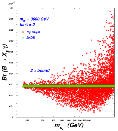
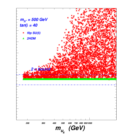
Figure 1: Comparison of $B\to X_{s}\gamma$ versus $m_{u_{x}}$ in the $\cal F$-$SU(5)$ model (red cross) and 2HDM (green triangle).

The numerical results of $B\to X_{s}\gamma$ as a function of the vector-like quark mass are displayed in Fig. 1. For the comparison, Fig. 1 also shows the results of the five-generation 2HDM. From this figure one can see some features clearly: (i) The new physics effects decouple when the charged Higgs boson is very heavy. However, for a much heavier charged Higgs, the branching ratio of $B\to X_{s}\gamma$ increases with $m_{u_{x}}$ in the $\cal F$-$SU(5)$ model while is almost independent on the extra quark mass in 2HDM, indicating the large non-decoupling effects; (ii) Unlike the 2HDM where the large $\tan\beta$ is preferred if the charged Higgs boson mass is at the EW scale, the small $\tan\beta$, which is excluded in 2HDM, is still survived in the $\cal F$-$SU(5)$ model; (iii) It is clear from the left plot of this figure that the branching ratio can be much bigger than the detection result when $m_{u_{x}}$ getting close to the charged Higgs boson mass. So the detection results of $B\to X_{s}\gamma$ can give stringent constraints on the $\cal F$-$SU(5)$ model. The tendency of the figure can be understood as following:

• $C_{7}$ determined by Eq. (27) in both $\cal F$-$SU(5)$ model and 2HDM BNP2HDM will approach to the SM value when the charged Higgs boson is much heavier than EW scale. Nevertheless, the contributions from the fourth and fifth generation up-type vector-like quarks in 2HDM can be suppressed by small $V^{5i}$ and $V^{4i}$ due to the unitarity condition of $5\times 5$ matrix;

• Because the summed indices are only from 1 to 4 in the $\cal F$-$SU(5)$ model, the unitary condition of the CKM matrix can not be maintained. When the vector-like particle mass approaches to the charged Higgs boson mass, the suppression from $5\times 5$ CKM mixing matrix will be released and then the non-decoupling effects will be sizable. In fact, the non-decoupling effects are a very special part of the $\cal F$-$SU(5)$ model at EW scale and can be tested at the LHC and other B physics detectors.

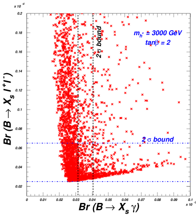
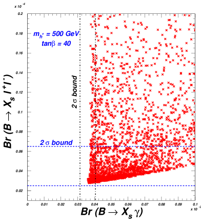
Figure 2: Branching ratio of $B\to X_{s}\ell^{+}\ell^{-}$ versus $B\to X_{s}\gamma$ in the $\cal F$-$SU(5)$ model.

Fig. 2 shows the branching ratio of $B\to X_{s}\ell^{+}\ell^{-}$ versus $B\to X_{s}\gamma$ in the $\cal F$-$SU(5)$ model. Clearly, both processes will give stringent constraints on our model. Especially, most part of the points are excluded when the charged Higgs boson is several hundred GeV, leaving a narrow part in the parameter space. Similar phenomenology can be seen in Fig. 3 which shows branching ratios of $B_{s}\to\mu^{+}\mu^{-}$ versus $B\to X_{s}\ell^{+}\ell^{-}$. The non-decoupling effects can be stringently constrained by the experiments as expected. Here we should emphasize that the upper bounds from the Tevatron and the first LHCb constraints Aaij:2012kn , which are about one order of magnitude above the SM expectation, as well as the recent CDF results of $B_{s}\to\mu^{+}\mu^{-}$ detection Aaltonen:2011fi can be explained naturally. It is interesting to see that there is an approximate linear relation between branching ratios of $B_{s}\to\mu^{+}\mu^{-}$ and $B\to X_{s}\ell^{+}\ell^{-}$. In fact, we find that in the allowed parameter space with $U_{d}\simeq V_{d}^{\dagger}$, the dominant contributions to both processes come from $C_{i}$ and $C_{i}^{{}^{\prime}}(i=9,10)$. From Eqs. (28) to (31), we can easily draw the conclusion that the branching ratios are nearly proportional to $|C_{10}^{{}^{\prime}}|^{2}$.

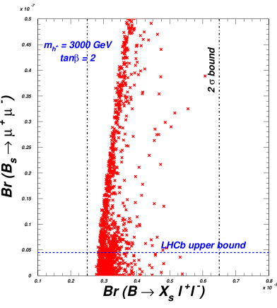
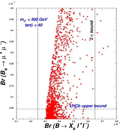
Figure 3: Branching ratios of $B_{s}\to\mu^{+}\mu^{-}$ versus $B\to X_{s}\ell^{+}\ell^{-}$ in the $\cal F$-$SU(5)$ model.

To see whether there are solutions simultaneously satisfied with the allowed ranges for these data, we can offer now some predications for $B_{s}\to\ell^{+}\ell^{-}\gamma$, which might be measured at the LHCb and B factories. The numerical results are illustrated in Fig. 4. We can see clearly that under the constraints from the inclusive decays $B\to X_{s}\gamma$ and $B\to X_{s}\ell^{+}\ell^{-}$, exclusive decays $B_{s}\to\mu^{+}\mu^{-}$, as well as CKM measurements extracted by the tree-level B decays, the branching ratio, which is very sensitive to $\tan\beta$ and charged Higgs boson mass, can still be up to $(4\sim 5)\times 10^{-8}$. Thus, it may be tested by the LHCb soon.

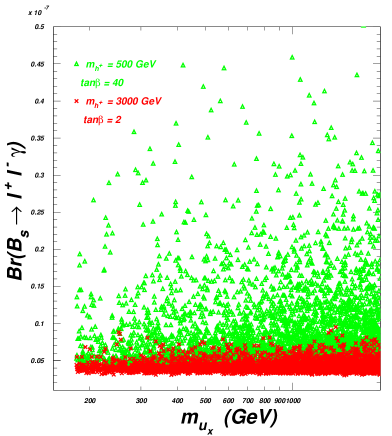
Figure 4: Branching ratio of $B_{s}\to\ell^{+}\ell^{-}\gamma$ with the combained constraints from $B\to X_{s}\gamma$, $B\to X_{s}\ell^{+}\ell^{-}$ and $B_{s}\to\mu^{+}\mu^{-}$. Red cross stands for the type inputs ($\tan\beta=2,~{}~{}m_{h^{+}}={3000\rm GeV}$) and green triangle for ($\tan\beta=40,~{}~{}m_{h^{+}}={500\rm GeV}$) in the $\cal F$-$SU(5)$ model, respectively.

Rare B decays continue to be the valuable probes of physics beyond the SM. In the current early phase of the LHC era, the exclusive modes with muons in the final states are among the most promising decays. The decay $B_{s}\to\mu^{+}\mu^{-}$ is likely to be confirmed before the end of 2012 LHCb . If an enhancement beyond $10^{-8}$ and further non-decoupling effects are observed, we will have an indication of the $\cal F$-$SU(5)$ model. Although there are some theoretical challenges including calculation of the hadronic form factors and non-factorable corrections, $B_{s}\to\ell^{+}\ell^{-}\gamma$ can be expected as the next goal once $B_{s}\to\mu^{+}\mu^{-}$ measurement is finished since the final states can be identified easily and branching ratios are large. Our predictions for such processes can be tested in the near future.

V Summary

In this paper, we studied the vector-like quark contributions to B physics processes in the $\cal F$-$SU(5)$ model, including the quark mass spectra, Feynman rules, the new operators in low energy effective theory and the correspondence Wilson coefficients, etc. As for the first time study, we focus on the implication of mass scale of vector like quark. The main conclusions we obtained are the following:

1. There exists the $\overline{s}bZ$ interaction at tree level, and the Yukawa interactions are changed. The new operators $O_{9}^{\prime}$ and $O_{10}^{\prime}$ must be introduced in effective Hamiltonian, and the Wilson coefficients are changed due to the violation of the unitarity condition.

2. Different from many previous models, the effects of vector-like quarks on rare B decays such as $B\to X_{s}\gamma$ and $B\to X_{s}\ell^{+}\ell^{-}$ do not decouple in some allowed parameter space, especially when the vector-like quark mass is comparable to the charged Higgs boson mass.

3. Under the constraints from $B\to X_{s}\gamma$ and $B\to X_{s}\ell^{+}\ell^{-}$, there exist scenarios in the model the latest measurement for $B_{s}\to\mu^{+}\mu^{-}$ can be explained naturally, and the branching ratio of $B_{s}\to\ell^{+}\ell^{-}\gamma$ can be up to $(4\sim 5)\times 10^{-8}$.

All in all, due to the participation of vector-like particles, the $\cal F$-$SU(5)$ model is different from the ordinary models such as 2HDM. In particular, the non-decouling effects are much more predictable and may be tested in the near future experiments. Finally, we should note that the large input parameter space and the sparticle effects in the $\cal F$-$SU(5)$ model needs further work.

Appendix

The loop functions for calculating the Wilson coefficients at the matching scale are the following

$$A(x) = \frac{5x+38x^{2}-55x^{2}}{36(x-1)^{3}}+\frac{4x-17x^{2}+15x^{3}}{6(x-1)^{4}}\ln x,$$

$$B(x) = \frac{x+x^{2}}{4(x-1)^{2}}-\frac{x^{2}}{2(x-1)^{3}}\ln x,$$

$$C(x) = \frac{20-19x+5x^{2}}{18(x-1)^{3}}+\frac{-2+x}{3(x-1)^{4}}\ln x$$

$$D(x) = \frac{-5-5x+4x^{2}}{12(x-1)^{3}}+\frac{2x-x^{2}}{2(x-1)^{4}}\ln x,$$

$$P(x) = \frac{-x}{4(x-1)}+\frac{x}{4(x-1)^{2}}\ln x~{},$$

$$Q(x) = \frac{x^{2}-6x}{8(x-1)}+\frac{3x^{2}+6x}{8(x-1)^{2}}\ln x~{},$$

$$R(x) = \frac{31x^{2}+20x^{3}}{9(x-1)^{3}}+\frac{-4+18x-30x^{2}+6x^{3}}{9(x-1)^{4}}\ln x,$$

$$S(x) = \frac{38-79x+47x^{2}}{108(x-1)^{3}}+\frac{-4x+6x^{2}-3x^{4}}{18(x-1)^{4}}\ln x,$$

$$T(x) = \frac{x-5x^{2}-2x^{3}}{12(x-1)^{3}}+\frac{x^{3}}{2(x-1)^{4}}\ln x.$$ (39)

References

- (1) J. R. Ellis, S. Kelley and D. V. Nanopoulos, Phys. Lett. B 260, 131 (1991); P. Langacker and M. X. Luo, Phys. Rev. D 44, 817 (1991); U. Amaldi, W. de Boer and H. Furstenau, Phys. Lett. B 260, 447 (1991); F. Anselmo, L. Cifarelli, A. Peterman and A. Zichichi, Nuovo Cim. A 104, 1817 (1991); Nuovo Cim. A 105, 1025 (1992).
- (2) J. R. Ellis, J. S. Hagelin, D. V. Nanopoulos, K. A. Olive, M. Srednicki, Nucl. Phys. B238, 453-476 (1984).
- (3) H. Goldberg, Phys. Rev. Lett. 50, 1419 (1983).
- (4) S. M. Barr, Phys. Lett. B 112, 219 (1982).
- (5) J. P. Derendinger, J. E. Kim and D. V. Nanopoulos, Phys. Lett. B 139, 170 (1984).
- (6) I. Antoniadis, J. R. Ellis, J. S. Hagelin and D. V. Nanopoulos, Phys. Lett. B 194, 231 (1987).
- (7) J. Jiang, T. Li and D. V. Nanopoulos, Nucl. Phys. B 772, 49 (2007).
- (8) I. Antoniadis, J. R. Ellis, J. S. Hagelin and D. V. Nanopoulos, Phys. Lett. B 208, 209 (1988) [Addendum-ibid. B 213, 562 (1988)]; Phys. Lett. B 231, 65 (1989).
- (9) J. L. Lopez, D. V. Nanopoulos and K. J. Yuan, Nucl. Phys. B 399, 654 (1993).
- (10) C. Beasley, J. J. Heckman and C. Vafa, JHEP 0901, 058 (2009); JHEP 0901, 059 (2009); R. Donagi and M. Wijnholt, arXiv:0802.2969 [hep-th]; arXiv:0808.2223 [hep-th].
- (11) J. Jiang, T. Li, D. V. Nanopoulos and D. Xie, Phys. Lett. B 677, 322 (2009); Nucl. Phys. B 830, 195 (2010).
- (12) K. Nakamura, Int. J. Mod. Phys. A 18, 4053 (2003).
- (13) S. Raby et al., arXiv:0810.4551 [hep-ph].
- (14) T. Li, D. V. Nanopoulos and J. W. Walker, Phys. Lett. B 693, 580 (2010).
- (15) T. Li, D. V. Nanopoulos and J. W. Walker, Nucl. Phys. B 846, 43 (2011) [arXiv:1003.2570 [hep-ph]].
- (16) B. Kyae and Q. Shafi, Phys. Lett. B 635, 247 (2006) [arXiv:hep-ph/0510105].
- (17) Y. Huo, T. Li, D. V. Nanopoulos and C. Tong, arXiv:1109.2329 [hep-ph].
- (18) T. Li, J. A. Maxin, D. V. Nanopoulos and J. W. Walker, Phys. Lett. B 710, 207 (2012) [arXiv:1112.3024 [hep-ph]].
- (19) E. Cremmer, S. Ferrara, C. Kounnas and D. V. Nanopoulos, Phys. Lett. B 133, 61 (1983); J. R. Ellis, A. B. Lahanas, D. V. Nanopoulos and K. Tamvakis, Phys. Lett. B 134, 429 (1984); J. R. Ellis, C. Kounnas and D. V. Nanopoulos, Nucl. Phys. B 241, 406 (1984); Nucl. Phys. B 247, 373 (1984); A. B. Lahanas and D. V. Nanopoulos, Phys. Rept. 145, 1 (1987).
- (20) T. Li, J. A. Maxin, D. V. Nanopoulos and J. W. Walker, Phys. Rev. D 83, 056015 (2011) [arXiv:1007.5100 [hep-ph]].
- (21) T. Li, J. A. Maxin, D. V. Nanopoulos and J. W. Walker, Phys. Lett. B 699, 164 (2011) [arXiv:1009.2981 [hep-ph]].
- (22) T. Li, J. A. Maxin, D. V. Nanopoulos and J. W. Walker, arXiv:1202.0509 [hep-ph].
- (23) A. Soni, A. K. Alok, A. Giri, R. Mohanta and S. Nandi, Phys. Rev. D 82, 033009 (2010); A. J. Buras, B. Duling, T. Feldmann, T. Heidsieck, C. Promberger and S. Recksiegel, JHEP 1009, 106 (2010); O. Eberhardt, A. Lenz and J. Rohrwild, Phys. Rev. D 82, 095006 (2010); Z. H. Xiong, High Energy Phys. Nucl. Phys. 30, 284 (2006).
- (24) A. J. Buras, M. Misiak, M. Münz and S. Pokorski, Nucl. Phys. B 424, 374 (1994).
- (25) M. Misiak, et al., Phys. Rev. Lett. 98, 022002 (2007). T. Hurth, Rev. Mod. Phys. 75, 1159 (2003); C. Bobeth, P. Gambino, M. Gorbahn and U. Haisch, JHEP 0404, 071 (2004); A. Ghinculov, T. Hurth, G. Isidori and Y. P. Yao, Nucl. Phys. B 685, 351 (2004); H. H. Asatryan, H. M. Asatrian, C. Greub and M. Walker, Phys. Rev. D 65, 074004 (2002).
- (26) P. H. Chankowski and Ł. Sławianowska, Phys. Rev. D 63, 054012 (2001); P. L. Cho, M. Misiak and D. Wyler, Phys. Rev. D 54, 3329 (1996); Y. Grossman, Z. Ligeti and E. Nardi, Phys. Rev. D 55, 2768 (1997); J. L. Hewett and J. D. Wells, Phys. Rev. D 55, 5549 (1997); S. Bertolini, F. Borzumati, A. Masiero and G. Ridolfi, Nucl. Phys. B 353, 591 (1991); A. J. Buras and M. Münz, Phys. Rev. D 52, 186 (1995); M. Ciuchini, G. Degrassi, P. Gambino and G. F. Giudice, Nucl. Phys. B 527, 21 (1998); C. -S. Huang, W. Liao and Q. -S. Yan, Phys. Rev. D 59, 011701 (1999); C. -S. Huang and S. -H. Zhu, Phys. Rev. D 61, 015011 (2000); C. -S. Huang, W. Liao, Q. -S. Yan and S. -H. Zhu, Phys. Rev. D 63, 114021 (2001); Eur. Phys. J. C 25, 103 (2002); S. R. Choudhury and N. Gaur, Phys. Lett. B 451, 86 (1999).
- (27) B. Grinstein, R. P. Springer and M. B. Wise, Phys. Lett. B 202, 138 (1988); B. Grinstein, R. P. Springer and M. B. Wise, Nucl. Phys. B 339, 269 (1990); Y. -B. Dai, C. -S. Huang and H. -W. Huang, Phys. Lett. B 390, 257 (1997); J. L. Hewett, Phys. Rev. D 53, 4964 (1996); H. E. Logan and U. Nierste, Nucl. Phys. B 586, 39 (2000); C. Bobeth, T. Ewerth, F. Kruger and J. Urban, Phys. Rev. D 64, 074014 (2001); G. Erkol and G. Turan, Phys. Rev. D 65, 094029 (2002); G. K. Yeghiyan, Mod. Phys. Lett. A 16, 2151 (2001); A. Diaz Rodolfo, R. Martinez and J. A. Rodriguez, Phys. Rev. D 64, 033004 (2001); R. Diaz, R. Martinez and J. A. Rodriguez, Phys. Rev. D 63, 095007 (2001); S. Davidson and H. E. Haber, Phys. Rev. D 72, 035004 (2005); L. Wolfenstein and Y. L. Wu, Phys. Rev. Lett. 73, 2809 (1994); T. M. Aliev and M. Savci, Phys. Lett. B 452, 318 (1999).
- (28) D. Asner et al. [Heavy Flavor Averaging Group Collaboration] and updates at http://www.slac.stanford.edu/xorg/hfag/
- (29) S. Chatrchyan et al. [CMS Collaboration], arXiv:1203.3976 [hep-ex].
- (30) Z. Heng, R. J. Oakes, W. Wang, Z. Xiong and J. M. Yang, Phys. Rev. D 77, 095012 (2008); Z. Xiong and J. M. Yang, Nucl. Phys. B 628, 193 (2002); G. Buchalla and A. J. Buras, Nucl. Phys. B 400, 225 (1993); D. -S. Du, C. Liu and D. -X. Zhang, Phys. Lett. B 317, 179 (1993).
- (31) K. de Bruyn, R. Fleischer, R. Knegjens, P. Koppenburg, M. Merk, A. Pellegrino and N. Tuning, arXiv:1204.1737 [hep-ph].
- (32) G. Eilam, I. E. Halperin and R. R. Mendel, Phys. Lett. B 361, 137 (1995).
- (33) R. Aaij et al. [LHCb Collaboration], Phys. Lett. B 707, 349 (2012) [arXiv:1111.0521 [hep-ex]]; Phys. Lett. B 699, 330 (2011), arXiv:1203.4493 [hep-ex].
- (34) K. Nakamura et al. (Particle Data Group), J. Phys. G 37, 075021 (2010) and 2011 partial update for the 2012 edition.
- (35) T. Aaltonen et al. [CDF Collaboration], Phys. Rev. Lett. 107, 239903 (2011) [Phys. Rev. Lett. 107, 191801 (2011)] [arXiv:1107.2304 [hep-ex]].
- (36) Talk by M. Palutan at Beauty 2011, Amsterdam, April 5, (2011).