Interference between competing pathways in atomic harmonic generation

Abstract

We investigate the influence of the autoionizing $3s3p^{6}n\ell$ resonances on the fifth harmonic generated by 200 - 240 nm laser fields interacting with Ar. To determine the influence of a multi-electron response we have developed capability within time dependent $R$-matrix theory to determine the harmonic spectra generated. The fifth harmonic is affected by interference between the response of a $3s$ electron and the response of a $3p$ electron, as demonstrated by the asymmetric profiles in the harmonic yields as functions of wavelength.

Harmonic generation (HG) is one of the fundamental processes that can occur in light-matter interaction. The process is of strong technological interest, since it lies at the heart of ultra-short light pulse generation Paul et al. (2001). However, HG can also be used as a measurement tool, for example, to study molecular changes on the sub-femtosecond timescale Baker et al. (2006). Recent articles have postulated various other applications of high harmonics, including electron interferometry and the tomographic imaging of electron orbitals Corkum (2011). HG has also been used experimentally to demonstrate the importance of electron-correlation in ultra-fast molecular dynamics Smirnova et al. (2009) and multi-electron dynamics in atomic systems Shiner et al. (2011).

In order to probe the influence of multi-electron dynamics on HG theoretically, we find it more expedient to consider atomic systems. Although detailed calculations for molecules are possible using sophisticated codes, it is much more difficult to identify the multi-electron dynamics within a molecular system than within an atomic system. Even so, many methods developed for the determination of harmonic spectra in atoms rely on the single active electron approximation Kulander et al. (1992); Schafer and Kulander (1997). Several methods have been developed for the description of two-electron systems Parker et al. (2006); Lambropoulos et al. (1998), but these methods are not easy to extend to general atoms. New methods are thus needed to gain insight into the influence of multi-electron dynamics on harmonic spectra in general multi-electron atoms.

At Queen’s University Belfast we have developed time-dependent R-matrix (TDRM) theory over the last five years expressly to study the behavior of multi-electron atoms in short, intense light fields Lysaght et al. (2009a). The advantage of this method in studying multi-electron dynamics was shown in a pump-probe study of C⁺ Lysaght et al. (2009b): by varying the delay between the pump and probe pulses, oscillations in the total ionization yield were observed, which could be linked to the correlated motion of two electrons. Because of the interest in using harmonic spectra to observe multi-electron dynamics, we have developed capability within the time-dependent R-matrix approach to determine harmonic spectra for a single atom.

As a first demonstration of this capability, we report on the influence of the $3s3p^{6}n\ell$ Rydberg series on single atom harmonic spectra in Ar. In particular, we focus on the wavelength range for which the fifth harmonic coincides with these resonances: 200 - 240 nm. Recent studies have focused on the parallels between photoionization and HG Wörner et al. (2009); Higuet et al. (2011), where, in particular, the Cooper minimum in Ar was investigated. However, minima in the photoionization cross section can also occur near window resonances, where resonances actually lead to a decrease in the photoionization cross section. The $3s3p^{6}n\ell$ resonances are examples of window resonances Madden et al. (1969). Their decay towards $3s^{2}3p^{5}\varepsilon\ell^{\prime}$ continua requires a good description of dielectronic repulsion. The harmonic yield will be determined by two interfering pathways, (Fig. 1): excitation of a $3s$ electron to $np$, and excitation of a $3p$ electron into the continuum. A multi-electron calculation is essential to describe the harmonic yield accurately. This study thus provides a good test case.

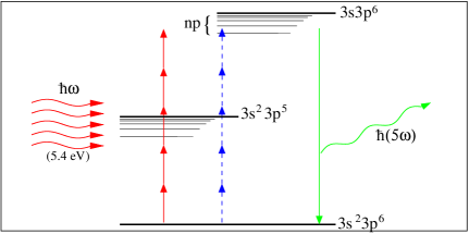
Figure 1: (Color online) The harmonic yield in Argon is determined by two competing pathways: absorption of at least three photons can excite a $3p$ electron (red solid line) into the continuum, while absorption of at least five photons can excite a $3s$ (blue dashed line) electron to the $np$ Rydberg series converging onto the $3s3p^{6}$ threshold.

To describe the extension to compute a system’s harmonic response, we first give a brief overview of TDRM theory. A more thorough discussion can be found in Lysaght et al. (2009a). The time-dependent Schrödinger equation for an atom containing ($N+1$) electrons, and nuclear charge $Z$, is

$$i\frac{\partial}{\partial t}\Psi\left(\mathbf{X}_{N+1},t\right)=H\left(t\right)\Psi\left(\mathbf{X}_{N+1},t\right).$$ (1)

The Hamiltonian, $H$, contains both the non-relativistic Hamiltonian of the $N+1$-electron atom or ion in the absence of the laser field and the laser interaction term. The laser field is described using the dipole approximation in the length form, and is assumed to be linearly polarized and spatially homogeneous. This form provides the most reliable ionization yields when only a limited amount of atomic structure is included Hutchinson et al. (2010).

To propagate the wave function in time, time is discretized into steps of $\Delta t$ such that

$$t_{q}=q\Delta t,\mbox{\hskip 14.22636pt}q=0,1,2,\ldots.$$ (2)

Then, using the unitary Cayley form of the time evolution operator, $\exp\left[-itH\left(t\right)\right]$, the wavefunction $\Psi$ in Eq. (1) at $t_{q+1}$ can be written in terms of the wavefunction at $t_{q}$

$$\left[H\left(t_{q+1/2}\right)-E\right]\Psi\left(\mathbf{X}_{N+1},t_{q+1}\right)=\mathbf{\Theta}\left(\mathbf{X}_{N+1},t_{q}\right),$$ (3)

where

$$\mathbf{\Theta}\left(\mathbf{X}_{N+1},t_{q}\right)=-\left[H\left(t_{q+1/2}\right)+E\right]\Psi\left(\mathbf{X}_{N+1},t_{q}\right),$$ (4)

and $H\left(t_{q+1/2}\right)$ is the time-dependent Hamiltonian at the midpoint. $E$ is given by $2i/\Delta t$. In equations (3) and (4) $\mathbf{X}_{N+1}=\mathbf{r}_{1}\sigma_{1},\mathbf{r}_{2}\sigma_{2},\cdots,\mathbf{r}_{N+1}\sigma_{N+1}$ where $\mathbf{r}_{i}\sigma_{i}$ are the space and spin coordinates of the $i$^th electron. If the wavefunction at time $t=t_{q}$ is known, then Eq. (3) allows us to propagate the solution forward in time.

In $R$-matrix theory, configuration space is partitioned into two regions: an inner and an outer region. In the inner region, all electrons are within a distance $a_{\mathrm{in}}$ of the nucleus, and all interactions between all electrons are taken into account. In the outer region, one electron has moved beyond a distance $a_{\mathrm{in}}$, and exchange interactions between this electron and the electrons remaining close to the nucleus can be neglected. The outer electron thus experiences only the long-range multipole potential of the residual $N$-electron core and the laser field.

In the outer region, $a_{\mathrm{in}}\leq r_{N+1}\leq a_{\mathrm{out}}$, we have

$$\Psi\left(\mathbf{X}_{N+1},t_{q+1}\right)=$$ (5)

$$\sum\limits^{n}_{p=1}\bar{\Phi}^{\gamma}_{p}\left(\mathbf{X}_{N};\hat{\mathbf{r}}_{N+1}\sigma_{N+1}\right)r^{-1}_{N+1}F_{p}\left(r_{N+1}\right),$$

where $\bar{\Phi}^{\gamma}_{p}$ are channel functions which couple possible final states of the Ar⁺ ion with spin and angular momentum of the ejected electron. The $F_{p}$ are the radial wavefunctions which describe the motion of the ejected electron in the $p$^th channel, where $p$ is a channel index.

We can now follow $R$-matrix procedures van der Hart et al. (2007) to evaluate Eq. (3) at the boundary $a_{\mathrm{in}}$ as a matrix equation

$$\mathbf{F}\left(a_{\mathrm{in}}\right)=\mathbf{R}(a_{\mathrm{in}})\bar{\mathbf{F}}\left(a_{\mathrm{in}}\right)+\mathbf{T}\left(a_{\mathrm{in}}\right),$$ (6)

in which the wavefunction at the boundary is described in terms of its derivative, $\bar{\mathbf{F}}$, plus an inhomogeneous vector, ${\mathbf{T}}$, arising from the $\Theta$ term in Eq. (3). Equation (6) connects the inner and outer region wavefunction at the boundary $a_{\mathrm{in}}$.

Given an initial inner region wavefunction, $\mathbf{R}$ and $\mathbf{T}$ are evaluated at the boundary. Subsequently, they are propagated outwards in space up to a boundary, $a_{\mathrm{out}}$ where it can be assumed that the wavefunction $\mathbf{F}$ has vanished. The wavefunction vector $F$ is set to zero and then propagated inwards to the inner region boundary. Once the $F$-vector has been determined at each boundary point, the full wavefunction can be extracted from the $R$-matrix equations. Equation (3) then allows us to step this solution forward in time.

HG arises from the oscillating dipole moment induced by the laser field. This is given by the expectation value of the electric dipole operator,

$$\mathbf{d}\left(t\right)=\langle\Psi\left(t\right)|-e\mathbf{Z}|\Psi\left(t\right)\rangle,$$ (7)

where $e$ is the electronic charge and Z the total position operator along the laser polarization axis. The power spectrum of the emitted radiation is then given by the Fourier transform of either the dipole moment, its velocity or acceleration Baggesen and Madsen (2011). Many techniques involving high order harmonics use the acceleration representation as it gives better resolution for the high-order peaks Jiang (1991). However, this has predominantly been verified for single-active-electron systems, whereas in the multi-electron TDRM method the length form of the dipole operator has proven to be far more reliable Hutchinson et al. (2010).

To describe Ar, we use the $R$-matrix basis developed for single photon-ionization Burke and Taylor (1975) with an inner region radius of 20 a.u. The set of continuum orbitals contains 60 $B$-splines for each angular momentum, $\ell$, of the continuum electron. We use both the $3s^{2}3p^{5}\mbox{ }^{2}P^{o}$ and $3s3p^{6}\mbox{ }^{1}P^{o}$ states of Ar⁺ as target states. The description of Ar includes all $3s^{2}3p^{5}\epsilon\ell$ and $3s3p^{6}\epsilon\ell$ channels up to $L_{max}=15$. In the outer region we propagate $\mathbf{R}$ and $\mathbf{T}$ out to a radial distance of 1600 a.u. to prevent any reflections of the wavefunction from the outer region boundary. The outer region is divided into sectors of width 2 a.u. and each sector contains 35 $B$-splines of order $k=9$ per channel. We use similar pulse shapes to those used in Lysaght et al. (2009a): a 3 cycle $\sin^{2}$ turn on/off for the electric field. Peak intensity is set at $2\times 10^{13}\mbox{ }\mathrm{Wcm}^{-2}$ with varying numbers of cycles at peak intensity; the time step is 0.1 a.u.

Figure 2 shows a typical power spectrum obtained for an incident pulse with a photon energy of 5.4 eV and 25 cycles at peak intensity. As well as the three harmonic peaks, several other features are visible. The sideband structure of the harmonic peaks is due to the turn on/off of the laser pulse. In the photon energy region between 12.1-15.2 eV, several peaks are observed arising from the $3s^{2}3p^{5}n\ell$ Rydberg series: $4s$ at 12.1 eV, the $5s/3d$ manifold at 14.5 eV and the $4d/6s$ at 15.1 eV. Higher manifolds are not separated at this pulse length. The third harmonic peak is clearly visible; it lies just above the $3s^{2}3p^{5}$ threshold of Ar⁺. Its proximity to the threshold may mean that it still overlaps the Rydberg series leading up to this threshold. The peak at 18.8 eV cannot be associated directly with any atomic structure but this energy corresponds to the energy of $3s^{2}3p^{5}4p$ plus one 5.4 eV photon. Finally, the fifth harmonic is visible at an energy of 26.9 eV.

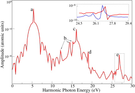
Figure 2: (Color online) The power spectrum produced by a 25 cycle, $2\times 10^{13}\mbox{ }\mathrm{Wcm}^{-2}$ laser pulse of photon energy 5.4eV. The features labelled are (a) First harmonic peak, (b) Effects due to $3s^{2}3p^{5}n\ell$ Rydberg series, (c) Third harmonic peak, (d) Peak due to $3s^{2}3p^{5}4p$ states plus a photon, and (e) Fifth harmonic peak. Inset: The fifth harmonic region of the power spectra for two 25 cycle pulses of photon energy 5.36 eV (blue, dashed line), and 5.42 eV (red, solid line). The change in the profile of the peaks is typical of the presence of a resonance in between these two frequencies.

The power spectrum was compared with calculations carried out using the R-matrix Floquet (RMF) method Plummer and Noble (2002). Good agreement was found at 248nm for the first harmonic rate at intensities between 6.5 and $8.5\times 10^{12}\mbox{ }\mathrm{Wcm}^{-2}$. The RMF calculations also obtained third and fifth harmonic rates within the $3d/5s$ manifold. In RMF theory these states are separate, but this requires unfeasibly long pulses in TDRM theory. Thus no comparison is possible beyond the first harmonic.

The main interest in the present manuscript is the fifth harmonic, which is strongly influenced by the $3s3p^{6}n\ell$ Rydberg series. Photoionization experiments and calculations have demonstrated that the Rydberg series appears as window resonances Madden et al. (1969); Burke and Taylor (1975). Figure 2 also shows part of the power spectra at two distinct photo energies, 5.36 eV and 5.42 eV. The resonance profile in the harmonic spectrum changes significantly. This is typical when a resonance lies in between these two photon energies. In order to assess these changes, the fifth harmonic rate is determined over a range of photon energies. For each photon energy, we integrate the harmonic rate across the bandwidth of the harmonic peak. This approach yields the harmonic rates shown in Fig. 3. We can see resonances occurring at energies corresponding to the $3s3p^{6}4p$ and $3s3p^{6}5p$ states. Additional resonances may be present at higher photon energies, but the energy uncertainty makes their assessment difficult.

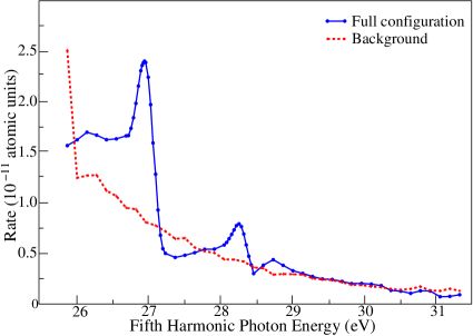
Figure 3: (Color online) The fifth harmonic rate for Ar in a 25 cycle pulse of varying frequency, for a target with the full configuration (blue, solid line) and one without any contribution from the $3s3p^{6}n/\varepsilon\ell$ series (red, dashed line). The resonances in the fifth harmonic rate correspond to the $3s3p^{6}4p$ (26.9eV) and $3s3p^{6}5p$ (28.3 eV) resonances.

In order to obtain resonance parameters, calculations are also performed with a reduced basis: a $3s^{2}3p^{5}$ single-target-state description of Ar⁺, and an Ar basis which contains no $3s3p^{6}n/\varepsilon\ell$ functions. This basis produces a smooth spectrum with a rate which can act as a background. Subtraction of this background rate then reveals a resonance profile due to the $3s3p^{6}n\ell$ Rydberg series, from which resonance parameters can be established. The resonance profile in Fig. 4 was obtained for 25 cycle pulses at an intensity of $2\times 10^{13}\mbox{ }\mathrm{Wcm}^{-2}$, giving, within an accuracy of 10%, an asymmetry parameter $q=-1.84$ and line width, $\Gamma=0.27$ eV.

The resonance parameters differ significantly from those obtained in previous photoionization calculations Burke and Taylor (1975). The present resonance width is about a factor 4 larger than obtained previously, 0.068 eV. This is not too surprising, since the present calculations are carried out only over a finite laser pulse, which gives rise to a broadening of the resonance. The effects of this broadening can be estimated by carrying out calculations for different pulse lengths. Table 1 indeed shows that the resonance width decreases with increasing laser pulse length. In addition, the resonance may also broaden due to the intensity of the laser pulse. At higher intensities states can photoionize as well as autoionize. This leads to a reduction in the lifetime of the state, and hence a broadening. This effect is shown in Table 2, where resonance parameters are compared as a function of peak intensity.

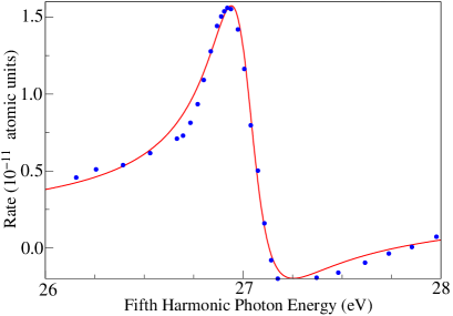
Figure 4: (Color online) The fifth harmonic resonance profile for Ar in a 25 cycle laser pulse of intensity $2\times 10^{13}\mbox{ }\mathrm{Wcm}^{-2}$. The data (blue points) is fitted by a Fano profile (red line) with asymmetry parameter, $q=-1.84$ and line width $\Gamma=0.27$ eV, and a linear background term.

Figure 4 shows that at the fifth-harmonic stage, the resonance has a strong effect on the harmonic yields. The strong interference between the continuum and the resonance leads to an asymmetric profile with harmonic yields increased below and decreased above the resonance energy. Both the continuum and the resonant pathway to HG must therefore be accounted for. As these pathways involve the response of different electrons, it shows that a multi-electron treatment of HG is necessary for Ar in the 200-240nm wavelength range.

Table 1 shows that the asymmetry parameter is not affected significantly by the pulse duration. On the other hand, Table 2 shows that this parameter changes noticeably with the intensity of the laser pulse. This knowledge is important for modelling the harmonic response of a macroscopic system and the appearance of resonances over a particular energy distribution. However, it is difficult to analyze the parameter changes in detail. At an intensity of $5\times 10^{13}\mbox{ }\mathrm{Wcm}^{-2}$ the ponderomotive shift of the ground state means that at the fifth-harmonic resonance, the third harmonic lies very close to the $3s^{2}3p^{5}$ threshold, and this may affect the profile.

In conclusion we have applied TDRM theory to study the appearance of the $3s3p^{6}n\ell$ autoionizing resonances in the fifth-harmonic for Ar. These window resonances show significant asymmetry within the fifth-harmonic spectrum, indicating interference between pathways involving the response of different electrons. This study provides a first demonstration of the new capability within time-dependent R-matrix theory to obtain harmonic spectra in multi-electron atoms with electron-electron correlation fully included. This extension may enable further evaluation of whether and how evidence of multi-electron dynamics can be found within harmonic spectra of atoms.

In the future, we hope to extend the approach to longer wavelengths and higher intensities. This will, however, require an assessment of the different gauges that can be used to obtain the harmonic spectrum, and extensive code development. The TDRM approach has proven its merit for strong-field ioniztion at wavelengths of 390nm at $4\times 10^{14}\mathrm{Wcm}^{-2}$ van der Hart et al. (2007). It will be of interest to export the determination of harmonic yields to the newly developed $R$-matrix with time-dependence codes Moore et al. (2011), which may be better suited for longer wavelengths.

ACB and SH acknowledge support from DEL NI under the programme for government. HWH is supported by G/055816/1 from the ESPRC. MAL acknowledges funding from the Numerical Algorithms Group (NAG) Ltd.

Table 1: The asymmetry parameters, line widths and positions for the resonance profiles due to $2\times 10^{13}\mbox{ }\mathrm{Wcm}^{-2}$ laser pulses of various lengths accurate to within $\sim$10%

Peak cycles	$q$ parameter	Line width (eV)	Position (eV)
10	-1.83	0.50	26.99
15	-1.82	0.40	27.01
20	-1.83	0.30	27.00
25	-1.84	0.27	27.01

Table 2: The asymmetry parameters, line widths and positions for the resonance profiles due to 25 cycle laser pulses of various intensities, accurate to within $\sim$10%

Intensity	$q$ parameter	Line width	Position
($10^{13}\mathrm{Wcm}^{-2}$)		(eV)	(eV)
2.0	-1.84	0.27	27.01
3.0	-1.79	0.30	27.08
5.0	-1.31	0.32	27.27

References

- Paul et al. (2001) P. M. Paul et al., Science 292, 1689 (2001).
- Baker et al. (2006) S. Baker et al., Science 312, 424 (2006).
- Corkum (2011) P. B. Corkum, Phys. Today 64, 36 (2011).
- Smirnova et al. (2009) O. Smirnova et al., Nature 460, 972 (2009).
- Shiner et al. (2011) A. D. Shiner et al., Nat. Phys. 7, 464 (2011).
- Kulander et al. (1992) K. C. Kulander et al., Atoms in Intense Radiation Fields, edited by M. Gavrila (Academic Press, New York, 1992), pp. 247–300.
- Schafer and Kulander (1997) K. J. Schafer and K. C. Kulander, Phys. Rev. Lett. 78, 638 (1997).
- Parker et al. (2006) J. S. Parker et al., Phys. Rev. Lett 96, 133001 (2006).
- Lambropoulos et al. (1998) P. Lambropoulos, P. Maragakis, and J. Zhang, Physics Reports 305, 203 (1998).
- Lysaght et al. (2009a) M. A. Lysaght, H. W. van der Hart, and P. G. Burke, Phys. Rev. A 79, 053411 (2009a).
- Lysaght et al. (2009b) M. A. Lysaght, P. G. Burke, and H. W. van der Hart, Phys. Rev. Lett. 102, 193001 (2009b).
- Wörner et al. (2009) H. J. Wörner et al., Phys. Rev. Lett 102, 103901 (2009).
- Higuet et al. (2011) J. Higuet et al., Phys. Rev. A 83, 053401 (2011).
- Madden et al. (1969) R. P. Madden, D. L. Ederer, and K. Codling, Phys. Rev. 177, 136 (1969).
- Hutchinson et al. (2010) S. Hutchinson, M. A. Lysaght, and H. W. van der Hart, J. Phys. B. At. Mol. Opt. Phys. 43, 095603 (2010).
- van der Hart et al. (2007) H. W. van der Hart, M. A. Lysaght, and P. G. Burke, Phys. Rev. A 76, 043405 (2007).
- Baggesen and Madsen (2011) J. C. Baggesen and L. B. Madsen, J. Phys. B. At. Mol. Opt. Phys. 44, 115601 (2011).
- Jiang (1991) T. F. Jiang, Phys. Rev. A. 46, 7332 (1991).
- Burke and Taylor (1975) P. G. Burke and K. T. Taylor, J. Phys. B. At. Mol. Opt. Phys. 8, 2620 (1975).
- Plummer and Noble (2002) M. Plummer and C. J. Noble, J. Phys. B. At. Mol. Opt. Phys. 35, L51 (2002).
- Moore et al. (2011) L. R. Moore et al., J. Mod. Optics 58, 1132 (2011).