A first passage problem for a bivariate diffusion process: numerical solution with an application to neuroscience.

Abstract

We consider a bivariate diffusion process and we study the first passage time of one component through a boundary. We prove that its probability density is the unique solution of a new integral equation and we propose a numerical algorithm for its solution. Convergence properties of this algorithm are discussed and the method is applied to the study of the integrated Brownian Motion and to the integrated Ornstein Uhlenbeck process. Finally a model of neuroscience interest is also discussed.

1 Introduction

First passage time problems arise in a variety of applications ranging from finance to biology, physics or psychology ([29, 20, 21] and examples cited therein). They have been largely studied (see [27] for a review on the subject): analytical [8, 9, 17, 19, 22, 26], numerical or approximate results [3, 4, 5, 6, 7, 23, 24, 30, 28] exist for specific classes of processes such as one dimensional diffusions or Gaussian processes. On the contrary, the case of bivariate processes has not been widely studied yet. Indeed, results are available only for specific problems such as the first exit time of the considered two-dimensional process from a specific surface [10, 14]. However there is a set of instances where the random variable of interest is the first passage time of one of the components of the bivariate process through a constant or a time dependent boundary. Examples of this type of problems are the First Passage Time (FPT) of integrated processes such as the Integrated Brownian Motion (IBM) or the Integrated Ornstein Uhlenbeck Process (IOU). Indeed, these one dimensional processes should be studied as bivariate processes if the Markov property has to be preserved. Recent examples of applications of the IBM or of the IOU processes have appeared in the metrological literature [18] where these processes are alternatively used to model the error of atomic clocks. In that case the crossing problem corresponds to the first attainment of an assigned value by the atomic clock error. Another application for this type of problems arises in neuroscience for the study of two-compartment models [15]. Indeed, the membrane potential evolution of two communicating parts of the neuron, the dendritic zone and the soma, can be depicted by a two-dimensional diffusion process, whose components describe the two considered zones. Furthermore, the time of a spike, i.e. the time when the membrane potential changes its dynamics with a sudden hyperpolarization, is described as the FPT of the second component through a boundary. Motivated by these applications, we consider the FPT of one component of a bivariate diffusion process through an assigned constant boundary, we prove an integral equation for this distribution and we propose a numerical algorithm for its solution. In Section 2 we introduce the notations and the necessary mathematical background. In Section 3 we present the new integral equation and the condition for the existence and uniqueness of its solution. In Section 4 we introduce a numerical algorithm for its solution and show its convergence properties. In Section 5 we illustrate the proposed numerical method through a set of examples, including the two-compartment model of a neuron. Finally in Section 6 we compare computational effort and reliability of the proposed numerical method with a totally simulation algorithm.

2 Notations and Mathematical Background

Let $\mathbf{X}(t)=\left(X_{1}(t),X_{2}(t)\right)^{\prime}$, $t\geq t_{0}$, be a two-dimensional diffusion process on $I\subseteq\mathbb{R}^{2}$ originated in $\mathbf{X}(t_{0})=\mathbf{y}$, where the superscript ^′ denotes the transpose of the vector. Let $s<t$, we denote with

$$f\left(\mathbf{x},t\left|\right.\mathbf{y},s\right)=\frac{\partial^{2}}{\partial x_{1}\partial x_{2}}\mathbb{P}\left(\mathbf{X}(t)\leq\mathbf{x}\left|\mathbf{X}(s)=\mathbf{y}\right.\right)$$ (1)

its transition probability density function, where $\mathbf{x}=(x_{1},x_{2})$ and $\mathbf{y}=(y_{1},y_{2})$.

In this paper we are concerned with the random variable FPT of the first component of the process $\mathbf{X}(t)$ through a boundary $S>y_{1}$:

$$T=\inf\left\{t\geq t_{0}:X_{1}(t)\geq S\right\}.$$

To describe $T$ we will use its probability density function

$$g\left(t\left|\mathbf{y},t_{0}\right.\right)=\frac{\partial}{\partial t}\mathbb{P}\left(T<t\left|\mathbf{X}(t_{0})=\mathbf{y}\right.\right).$$ (2)

Furthermore let $Z(t)$ be a random variable whose distribution coincides with the conditional distribution of $X_{2}(t)$ given $T=t$

$$\mathbb{P}\left(X_{2}(T)<z\left|T=t;\mathbf{X}(t_{0})=\mathbf{y}\right.\right).$$ (3)

We will also consider the joint distribution of $\left(X_{2}(T),T\right)$ and its probability density function

$$g_{c}\left((S,z),t\left|\mathbf{y},t_{0}\right.\right)=\frac{\partial^{2}}{\partial z\partial t}\mathbb{P}\left(X_{2}(T)<z,T<t\left|\mathbf{X}(t_{0})=\mathbf{y}\right.\right)\mbox{, }z\in\mathbb{R}\mbox{, }t\in[t_{0},\infty].$$ (4)

We denote with $\mathbb{E}_{X}(h(X))$ the expectation with respect to the probability measure induced by the random variable $X$. We skip the subscript if there is no possibility of misunderstanding. In the following theorem we link (1) with (4).

Theorem 1.

For $x_{1}>S$ it holds

$$\mathbb{P}\left(\mathbf{X}(t)>\mathbf{x}|\mathbf{X}(t_{0})=\mathbf{y}\right)$$ (5)

$$=\int_{t_{0}}^{t}d\vartheta\int_{-\infty}^{+\infty}g_{c}\left((S,z),\vartheta\left|\right.\mathbf{y},t_{0}\right)\mathbb{P}\left(\mathbf{X}(t)>\mathbf{x}|X_{1}(\vartheta)=S,X_{2}(\vartheta)=z\right)dz.$$

If the joint probability density function $f\left(\mathbf{x},t\left|\right.\mathbf{y},t_{0}\right)$ exists, it holds

$$f\left(\mathbf{x},t\left|\right.\mathbf{y},t_{0}\right)=\int_{t_{0}}^{t}d\vartheta\int_{-\infty}^{+\infty}g_{c}\left((S,z),\vartheta\left|\right.\mathbf{y},t_{0}\right)f\left(\mathbf{x},t\left|\right.(S,z),\vartheta\right)dz.$$ (6)

Proof.

Equation (5) is a consequence of the strong Markov property, as explained in the following.
Let $h:(S,\infty)\times\mathbb{R}\rightarrow\mathbb{R}$ be a bounded, Borel measurable function and let $\mathcal{F}_{T}$ be the $\sigma$-algebra generated by the process $\mathbf{X}(t)$ up to the random time $T$. We get

$$\mathbb{E}[h(\mathbf{X}(t))|\mathbf{X}(t_{0})=\mathbf{y}] = \mathbb{E}[\mathbb{E}[h(\mathbf{X}(t))|\mathcal{F}_{T};\mathbf{X}(t_{0})=\mathbf{y}]]$$

$$= \mathbb{E}[\mathbb{E}[h(\mathbf{X}(t))|\mathbf{X}(T)]]$$

$$= \int_{t_{0}}^{t}d\vartheta\int_{-\infty}^{+\infty}\mathbb{E}[h(\mathbf{X}(t))|\mathbf{X}(\vartheta)=(S,z)]g_{c}((S,z),\vartheta|\mathbf{y},t_{0})dz$$

where the first equality uses the double expectation theorem while the second one uses the strong Markov property. Choosing $h(\mathbf{y})=I_{\{x_{1},\infty\}\times\{x_{2},\infty\}}(\mathbf{y})$ we get (5). Finally, writing the conditional probability $\mathbb{P}\left(\mathbf{X}(t)>\mathbf{x}|X_{1}(\vartheta)=S,X_{2}(\vartheta)=z\right)$ as a double integral, changing the order of integration and differentiating (5) with respect to $x_{1}$ and $x_{2}$ we get (6). ∎

Remark 1.

Equation (6) was introduced without proof in [10].

The transition probability density function (1) is known in a few instances. One of these cases is a process solution of linear (in the narrow sense) stochastic differential equation [2]

$$\left\{\begin{array}[]{lr}d\mathbf{X}(t)=\left[\mathbf{A}(t)\mathbf{X}(t)+\mathbf{M}(t)\right]dt+\mathbf{G}(t)d\mathbf{B}(t),&\hskip 14.22636ptt\geq t_{0}\\ \\ \mathbf{X}(t_{0})=\mathbf{y}\end{array}\right.$$ (8)

where $\mathbf{A}(t)$ and $\mathbf{G}(t)$ are $2\times 2$ matrices, $\mathbf{M}$ is a vector of $2$ components and $\mathbf{B}(t)$ is a bivariate standard Brownian motion.
The solution of (8), corresponding to the initial value $\mathbf{y}$ at instant $t_{0}$, is

$$\mathbf{X}(t)=\mathbf{\phi}(t,t_{0})\left[\mathbf{y}+\int_{t_{0}}^{t}\mathbf{\phi}(u,t_{0})^{-1}\mathbf{M}(u)du+\int_{t_{0}}^{t}\mathbf{\phi}(u,t_{0})^{-1}\mathbf{G}(u)d\mathbf{B}(u)\right],$$ (9)

where $\mathbf{\phi}(t,t_{0})$ is the solution of the homogeneous matrix equation

$$\frac{d}{dt}\mathbf{\phi}(t,t_{0})=\mathbf{A}(t)\mathbf{\phi}(t,t_{0})\hskip 2.84526pt\mbox{ with }\hskip 2.84526pt\mathbf{\phi}(t_{0},t_{0})=\mathbf{I}\mbox{.}$$ (10)

For $t\in[0,\infty]$, the diffusion process has a two-dimensional normal distribution with expectation vector

$$\mathbf{m}(t\left|\mathbf{y},t_{0}\right.):=\mathbb{E}(\mathbf{X}(t)|\mathbf{X}(t_{0})=\mathbf{y})=\mathbf{\phi}(t,t_{0})\left[\mathbf{y}+\int_{t_{0}}^{t}\mathbf{\phi}(u,t_{0})^{-1}\mathbf{M}(u)du\right]$$ (11)

and $2\times 2$ conditional covariance matrix

$$\mathbf{Q}(t\left|\mathbf{y},t_{0}\right.)=\mathbf{\phi}(t,t_{0})\left[\int_{t_{0}}^{t}\mathbf{\phi}(u,t_{0})^{-1}\mathbf{G}(u)\mathbf{G}(u)^{{}^{\prime}}(\mathbf{\phi}(u,t_{0})^{-1})^{{}^{\prime}}du\right]\mathbf{\phi}(t,t_{0})^{{}^{\prime}},$$ (12)

where the superscript ^′ denotes the transpose of the matrix.

In the autonomous case ($\mathbf{A}(t)=\mathbf{A}$, $\mathbf{M}(t)=\mathbf{M}$ and $\mathbf{G}(t)=\mathbf{G}$), expressions (11) and (12) are simplified

$$\mathbf{m}(t\left|\mathbf{y},t_{0}\right.) = e^{\mathbf{A}(t-t_{0})}\left[\mathbf{y}+\int_{t_{0}}^{t}e^{-\mathbf{A}(u-t_{0})}\mathbf{M}du\right]$$ (13)

$$\mathbf{Q}(t\left|\mathbf{y},t_{0}\right.) = e^{\mathbf{A}(t-t_{0})}\left[\int_{t_{0}}^{t}e^{-\mathbf{A}(u-t_{0})}\mathbf{G}\mathbf{G}^{{}^{\prime}}e^{-\mathbf{A}^{{}^{\prime}}(u-t_{0})}du\right]e^{\mathbf{A}^{{}^{\prime}}(u-t_{0})}$$

$$= \int_{t_{0}}^{t}e^{\mathbf{A}(t-u)}\mathbf{G}\mathbf{G}^{{}^{\prime}}e^{\mathbf{A}^{{}^{\prime}}(t-u)}du.$$

For Gaussian or constant initial condition, the solution of (8) is itself a Gaussian process, frequently known as Gauss-Markov process.
Examples of Gauss-Markov processes are the Integrated Brownian Motion (IBM), the Integrated Ornstein Uhlenbeck Process (IOU). Also the underlying process of the two-compartment neural model [15] is a Gauss-Markov process.

If $\det\mathbf{Q}(t\left|\right.\mathbf{y},t_{0})\neq 0$ for each $t$, the probability density function $f\left(\mathbf{x},t\left|\right.\mathbf{y},t_{0}\right)$ of any two-dimensional Gauss-Markov process is

$$f\left(\mathbf{x},t\left|\right.\mathbf{y},t_{0}\right)=\frac{\exp\left\{-\frac{1}{2}\left[\mathbf{x}-\mathbf{m}(t\left|\mathbf{y},t_{0}\right.)\right]^{{}^{\prime}}\mathbf{Q}(t\left|\mathbf{y},t_{0}\right.)^{-1}\left[\mathbf{x}-\mathbf{m}(t\left|\mathbf{y},t_{0}\right.)\right]\right\}}{2\pi\sqrt{\det\mathbf{Q}(t\left|\right.\mathbf{y},t_{0})}}$$

and follows the Chapman-Kolmogorov equation [21].

3 An Integral Equation for the FPT Distribution

Let us consider a diffusion process $\left\{\mathbf{X}(t),t\geq 0\right\}$ originated in $\mathbf{y}=\mathbf{0}$ at $t_{0}=0$. It holds

Theorem 2.

If

$$\mathbb{P}\left(X_{1}(t)\geq S\left|X_{1}(\vartheta)=S,X_{2}(\vartheta)=z\right.\right)\mbox{ , }z\in\mathbb{R}\mbox{ , }\vartheta\in\left[0,t\right]$$ (15)

and its derivative with respect to $t$ are continuous in $0\leq\vartheta\leq t$, then the FPT probability density function is the solution of the following integral equation:

$$\mathbb{P}\left(X_{1}(t)\geq S\left|\mathbf{X}(0)=\mathbf{0}\right.\right)$$

$$= \int_{0}^{t}d\vartheta\;g\left(\vartheta\left|\right.\mathbf{0},0\right)\mathbb{E}_{Z(\vartheta)}\left[\mathbb{P}\left(X_{1}(t)\geq S\left|X_{1}(\vartheta)=S,X_{2}(\vartheta)\right.\right)\right]$$

where the distribution of $Z(\vartheta)$ is given by (3).
The solution of (2) exists and it is unique.

Proof.

Let us consider (5) with $x_{1}=S$ and $x_{2}=-\infty$, we get

$$\mathbb{P}\left(X_{1}(t)>S|\mathbf{X}(0)=\mathbf{0}\right)$$ (17)

$$=\int_{0}^{t}d\vartheta\int_{-\infty}^{+\infty}g_{c}\left((S,z),\vartheta\left|\right.\mathbf{0},0\right)\mathbb{P}\left(X_{1}(t)>S|X_{1}(\vartheta)=S,X_{2}(\vartheta)=z\right)dz.$$

Considering

$$\mathbb{P}\left(X_{2}(T)<z,T<t\left|\mathbf{X}(0)=\mathbf{0}\right.\right)=\int_{0}^{t}d\tau\;\mathbb{P}\left(X_{2}(\tau)<z\left|T=\tau,\mathbf{X}(0)=\mathbf{0}\right.\right)g\left(\tau\left|\mathbf{0},0\right.\right),$$

taking the derivatives with respect to $z$ and $t$, using (4), we get

$$g_{c}\left((S,z),t\left|\mathbf{0},0\right.\right)=\frac{\partial}{\partial z}\mathbb{P}\left(X_{2}(T)<z\left|T=t;\mathbf{X}(0)=\mathbf{0}\right.\right)g\left(t\left|\mathbf{0},0\right.\right)\mbox{.}$$ (18)

Substituting (18) in (17) we get the integral equation (2). It is a first kind Volterra equation with regular kernel

$$k(t,\vartheta)=\mathbb{E}_{Z(\vartheta)}\left[\mathbb{P}\left(X_{1}(t)\geq S\left|X_{1}(\vartheta)=S,X_{2}(\vartheta)\right.\right)\right],$$

because $k(t,\vartheta)$ is bounded. In particular $k(t,t)$ does not vanish for any $t\geq 0$.
Due to the hypothesis (15), the kernel of the Volterra equation (2) and its derivative respect to $t$ are continuous for $0\leq\vartheta\leq t$.
Similarly, the left hand side of equation (2) and its derivative respect to $t$ are continuous for $t\geq 0$. Furthermore $\mathbb{P}\left(X_{1}(0)\geq S\left|\mathbf{0},0\right.\right)=0$.
Thus, applying Theorem 5.1 of [16], we get the existence and uniqueness of the solution. ∎

Corollary 3.

The first passage time probability density of a Gauss-Markov process (8) satisfies the following equation

$$1-\mbox{Erf}\left(\frac{S-m^{(1)}(t)}{\sqrt{2Q^{(11)}(t)}}\right)=$$ (19)

$$=\int_{0}^{t}d\vartheta g\left(\vartheta\left|\mathbf{0},0\right.\right)\mathbb{E}_{Z(\vartheta)}\left[1-\mbox{Erf}\left(\frac{S-m^{(1)}(t\left|\right.(S,X_{2}(\vartheta)),\vartheta)}{\sqrt{2Q^{(11)}(t\left|\right.(S,X_{2}(\vartheta)),\vartheta)}}\right)\right]\mbox{,}$$

where $m^{(1)}(t)=m^{(1)}(t\left|\right.\mathbf{0},0)$ denotes the first component of the vector (11), $Q^{(11)}(t)=Q_{t}^{(11)}(t\left|\right.\mathbf{0},0)$ denotes the element on the upper left corner of the matrix (12) and $\mbox{Erf}(x)$ denotes the error function [1].
The Volterra equation (19) admits a unique solution if

$$\frac{\partial}{\partial t}\left(\frac{S-m^{(1)}(t\left|\right.(S,z),\vartheta)}{\sqrt{2Q^{(11)}(t\left|\right.(S,z),\vartheta)}}\right)$$ (20)

is a continuous function of $t\geq\vartheta\geq 0$.

Proof.

Due to the Gaussianity of the process, we have

$$\mathbb{P}\left(X_{1}(t)\geq S\left|\mathbf{X}(t_{0})=\mathbf{y}\right.\right) = \int_{-\infty}^{+\infty}dx_{2}\int_{S}^{+\infty}dx_{1}f\left(\mathbf{x},t\left|\right.\mathbf{y},t_{0}\right)$$

$$= \frac{1}{2}\left(1-\mbox{Erf}\left(\frac{S-m^{(1)}(t\left|\right.\mathbf{y},t_{0})}{\sqrt{2Q^{(11)}(t\left|\right.\mathbf{y},t_{0})}}\right)\right)\mbox{.}$$

Replacing this result into (2), we obtain (19).

Since (20) is continuous for hypothesis, then

$$\frac{\partial}{\partial t}\mathbb{P}\left(X_{1}(t)\geq S\left|\mathbf{X}(t_{0})=\mathbf{y}\right.\right)=\frac{\partial}{\partial t}\frac{1}{2}\left(1-\mbox{Erf}\left(\frac{S-m^{(1)}(t\left|\right.\mathbf{y},t_{0})}{\sqrt{2Q^{(11)}(t\left|\right.\mathbf{y},t_{0})}}\right)\right)$$

$$=-\frac{1}{\sqrt{\pi}}\exp\left\{-\left(\frac{S-m^{(1)}(t\left|\right.\mathbf{y},t_{0})}{\sqrt{2Q^{(11)}(t\left|\right.\mathbf{y},t_{0})}}\right)^{2}\right\}\frac{\partial}{\partial t}\left(\frac{S-m^{(1)}(t\left|\right.\mathbf{y},t_{0})}{\sqrt{2Q^{(11)}(t\left|\right.\mathbf{y},t_{0})}}\right)\mbox{.}$$

is continuous. Thus applying Theorem 2 we get the existence and uniqueness of the solution of (19). ∎

Remark 2.

The term

$$\mathbb{P}\left(X_{1}(t)\geq S\left|X_{1}(\vartheta)=S,X_{2}(\vartheta)=z\right.\right)$$

represents the probability of being over the threshold $S$ after a time interval $(t-\vartheta)$, starting from the threshold itself. For a Gauss-Markov process it becomes

$$\mathbb{P}\left(X_{1}(t)\geq S\left|X_{1}(\vartheta)=S,X_{2}(\vartheta)=z\right.\right)=\frac{1}{2}\left[1-\mbox{Erf}\left(\frac{S-m^{(1)}(t\left|\right.(S,z),\vartheta)}{\sqrt{2Q^{(11)}(t\left|\right.(S,z),\vartheta)}}\right)\right]\mbox{.}$$

Thus under weak conditions of its well-definition, applying the l’Hopital’s rule, the following limit

$$\lim_{\vartheta\rightarrow t}\left\{1-\mbox{Erf}\left(\frac{S-m^{(1)}(t\left|\right.(S,z),\vartheta)}{\sqrt{2Q^{(11)}(t\left|\right.\vartheta,(S,z))}}\right)\right\}$$

assume a positive value $C\leq 2$. Then using the dominated convergence theorem we can conclude that

$$\lim_{\vartheta\rightarrow t}\mathbb{E}_{Z(\vartheta)}\left[1-\mbox{Erf}\left(\frac{S-m^{(1)}(t\left|\right.(S,X_{2}(\vartheta)),\vartheta)}{\sqrt{2Q^{(11)}(t\left|\right.(S,X_{2}(\vartheta)),\vartheta)}}\right)\right]=C.$$ (21)

Remark 3.

Note that the random variable $X_{2}(\vartheta)$, that appear in the expectation (21), has values on an interval $[a,b]$ that changes depending on the features of the process (8).

4 Gauss-Markov processes: a numerical algorithm

The complexity of equation (19) does not allow to get closed form solutions for $g$. Hence we pursue our study by introducing a numerical algorithm for its solution.

Let us consider the partition $t_{0}=0<t_{1}<\ldots<t_{N}=t$ of the time interval $[0,t]$ with step $h=t_{k}-t_{k-1}$ for $k=1,\ldots,N$.
Discretizing integral equation (19) via Euler method, we have:

$$1-\mbox{Erf}\left(\frac{S-m^{(1)}(t_{k})}{\sqrt{2Q^{(11)}(t_{k})}}\right)$$

$$= \sum_{j=1}^{k}\hat{g}\left(t_{j}\left|\mathbf{0},0\right.\right)\mathbb{E}_{Z(t_{j})}\left[1-\mbox{Erf}\left(\frac{S-m^{(1)}(t_{k}\left|\right.(S,X_{2}(t_{j})),t_{j})}{\sqrt{2Q^{(11)}(t_{k}\left|\right.(S,X_{2}(t_{j})),t_{j})}}\right)\right]h$$

for $k=1,\ldots,N$.

Equation (4) gives the following algorithm for the numerical approximation $\hat{g}\left(\tau\left|\mathbf{0},0\right.\right)$ of $g\left(\tau\left|\mathbf{0},0\right.\right)$, $\tau\in(0,t)$.

Step $1$

$$\hat{g}\left(t_{1}\left|\right.\mathbf{0},0\right)=\frac{1}{Ch}\left[1-\mbox{Erf}\left(\frac{S-m^{(1)}(t_{1})}{\sqrt{2Q^{(11)}(t_{1})}}\right)\right],$$

where $C$ is given by (21).

Step $k$, $k>1$

$$\hat{g}\left(t_{k}\left|\right.\mathbf{0},0\right) = \frac{1}{Ch}\left\{1-\mbox{Erf}\left(\frac{S-m^{(1)}(t_{k})}{\sqrt{2Q^{(11)}(t_{k})}}\right)\right\}$$

$$- \frac{1}{C}\sum_{j=1}^{k-1}\hat{g}\left(t_{j}\left|\right.\mathbf{0},0\right)\mathbb{E}_{Z(t_{j})}\left[1-\mbox{Erf}\left(\frac{S-m^{(1)}(t_{k}\left|\right.(S,X_{2}(t_{j})),t_{j})}{\sqrt{2Q^{(11)}(t_{k}\left|\right.(S,X_{2}(t_{j})),t_{j})}}\right)\right]\mbox{.}$$

Note that the first term on the r.h.s. is obtained for $j=k$.

To sum up, the FPT probability density function in the knots $t_{0},t_{1},\ldots,t_{N}$ is the solution of a linear system $\mathbf{L}\mathbf{\hat{g}}=\mathbf{b}$ where

$$\mathbf{b}=\left(\begin{array}[]{c}1-\mbox{Erf}\left(\frac{S-m^{(1)}(t_{1})}{\sqrt{2Q^{(11)}(t_{1})}}\right)\\ \vdots\\ 1-\mbox{Erf}\left(\frac{S-m^{(1)}(t_{N})}{\sqrt{2Q^{(11)}(t_{N})}}\right)\end{array}\right)\mbox{, }\hskip 4.2679pt\mathbf{\hat{g}}=\left(\begin{array}[]{c}\hat{g}\left(t_{1}\left|\right.\mathbf{0},0\right)\\ \vdots\\ \hat{g}\left(t_{N}\left|\right.\mathbf{0},0\right)\end{array}\right)$$

and

$$\mathbf{L}=\left(\begin{array}[]{ccccc}Ch\\ \theta_{2,1}h&Ch\\ \theta_{3,1}h&\theta_{3,2}h&Ch\\ \vdots&\vdots&&\ddots\\ \theta_{N,1}h&\theta_{N,2}h&\cdots&\cdots&Ch\end{array}\right),$$

with

$$\theta_{k,j}=\mathbb{E}_{Z(t_{j})}\left[1-\mbox{Erf}\left(\frac{S-m^{(1)}(t_{k}\left|(S,X_{2}(t_{j})),t_{j}\right.)}{\sqrt{2Q^{(11)}(t_{k}\left|(S,X_{2}(t_{j})),t_{j}\right.)}}\right)\right]$$ (24)

for $k=1,\ldots,N$ and $j=1,\ldots,k$.

To evaluate the expected value (24) for $k=1,\ldots,N$ and $j=1,\ldots,k$, we make use of the following Monte Carlo method.
We repeatedly simulate the bivariate process until the first component crosses the boundary and we collect the sequence $\left\{Z_{i},i=1,\ldots M\right\}$ of i.i.d random variables with probability distribution function (3) with $t=t_{j}$. Then we compute the sample mean

$$\hat{\theta}_{k,j}=1-\frac{\sum_{i=1}^{M}\mbox{Erf}\left(\frac{S-m^{(1)}(t_{k}\left|(S,Z_{i}),t_{j}\right.)}{\sqrt{2Q^{(11)}(t_{k}\left|(S,Z_{i}),t_{j}\right.)}}\right)}{M}\mbox{.}$$ (25)

Here $M$ is the sample size.

The following theorem proves that this algorithm converges. In order to simplify the notations of the theorem, let us first define

$$\psi(z;t_{k},t_{j}):=\mbox{Erf}\left(\frac{S-m^{(1)}(t_{k}\left|\right.(S,z),t_{j})}{\sqrt{2Q^{(11)}(t_{k}\left|\right.(S,z),t_{j})}}\right)$$

for $k=1,\ldots,N$, $j=1,\dots,k$. Then it holds

Theorem 4.

If the sample size $M$ for the Monte Carlo method is such that the error $|\lambda|=h^{2}$ at a confidence level $\alpha$ and if there exists a constant $a$, such that for all $h>0$

$$\max_{1\leq k\leq N,1\leq j\leq k-1}\mathbb{E}_{Z(t_{j})}\left[\psi(X_{2}(t_{j}),t_{k},t_{j})-\psi(X_{2}(t_{j}),t_{k-1},t_{j})\right]\leq ah,$$ (26)

then the error $\epsilon_{k}=\hat{g}\left(t_{k}\left|\right.\mathbf{0},0\right)-g\left(t_{k}\left|\right.\mathbf{0},0\right)$ of the proposed algorithm at the discretization knots $t_{k}$, for $k=1,2,\ldots$ is $\left|\epsilon_{k}\right|=O(h)$ at the same confidence level $\alpha$.

Proof.

The Euler method and the Monte Carlo method applied to (19) give

$$1-\mbox{Erf}\left(\frac{S-m^{(1)}(t_{k})}{\sqrt{2Q^{(11)}(t_{k})}}\right)=\sum_{j=1}^{k}h\hat{g}\left(t_{j}\left|\mathbf{0},0\right.\right)\hat{\theta}_{k,j}$$ (27)

while (19) can be rewritten as

$$1-\mbox{Erf}\left(\frac{S-m^{(1)}(t_{k})}{\sqrt{2Q^{(11)}(t_{k})}}\right)=\sum_{j=1}^{k}hg\left(t_{j}\left|\mathbf{0},0\right.\right)\left(\hat{\theta}_{k,j}+\lambda\right)+\delta(h,t_{k})$$ (28)

where $\delta(h,t_{k})$ denotes the error of Euler method and $\lambda$ indicates the error of the Monte Carlo method at confidence level $\alpha$.
Subtracting (28) from (27) we obtain

$$\delta(h,t_{k})=h\sum_{j=1}^{k}\left(\hat{\theta}_{k,j}\epsilon_{j}+\lambda g\left(t_{j}\left|\mathbf{0},0\right.\right)\right).$$ (29)

Differencing (29) and using (21), we get

$$\delta(h,t_{k})-\delta(h,t_{k-1})=h\sum_{j=1}^{k-1}\left(\hat{\theta}_{k,j}-\hat{\theta}_{k-1,j}\right)\epsilon_{j}+hC\epsilon_{k}+g\left(t_{k}\left|\mathbf{0},0\right.\right)\lambda$$

or equally

$$\epsilon_{k}=\frac{1}{Ch}\left[\delta(h,t_{k})-\delta(h,t_{k-1})\right]-\frac{1}{C}\sum_{j=1}^{k-1}\left(\hat{\theta}_{k,j}-\hat{\theta}_{k-1,j}\right)\epsilon_{j}-\frac{g\left(t_{k}\left|\mathbf{0},0\right.\right)\lambda}{hC}.$$

Then, due to the hypothesis (26) and to the large number law, choosing $M$ large enough, we have

$$\left|\epsilon_{k}\right|\leq\frac{1}{Ch}\left|\delta(h,t_{k})-\delta(h,t_{k-1})\right|+\frac{ah}{C}\sum_{j=1}^{k-1}\epsilon_{j}+\frac{g\left(t_{k}\left|\mathbf{0},0\right.\right)|\lambda|}{hC}.$$

Finally, observing that the error of Euler method is $\left|\delta(h,t)\right|=O(h^{2})$, choosing $M$ such that the error of the Monte Carlo method is $|\lambda|=h^{2}$ and applying Theorem 7.1 of [16], we get the thesis. ∎

Remark 4.

In the autonomous case, hypothesis (26) is verified.
Indeed

$$\psi\left(z;t_{k},t_{j}\right)-\psi\left(z;t_{k-1},t_{j}\right) = \frac{2}{\sqrt{\pi}}\int^{\beta\left((S,z),t_{k},t_{j}\right)}_{\beta\left((S,z),t_{k-1},t_{j}\right)}e^{-y^{2}/2}dy$$

$$\leq a_{1}\left[\beta\left((S,z),t_{k},t_{j}\right)-\beta\left((S,z),t_{k-1},t_{j}\right)\right]$$

where

$$\beta\left((S,z),t_{i},t_{l}\right)=\frac{S-m^{(1)}(t_{i}\left|\right.(S,z),t_{l})}{\sqrt{2Q^{(11)}(t_{i}\left|\right.(S,z),t_{l})}}$$

Using equation (2), we get that

$$Q^{(11)}(t_{k}\left|\right.(S,z),t_{j})=Q^{(11)}(t_{k-1}\left|\right.(S,z),t_{j})+\int_{0}^{h}e^{Au}\mathbf{M}\mathbf{M}^{{}^{\prime}}e^{A^{{}^{\prime}}u}du.$$

Hence inequality (4) becomes

$$\psi\left(z;t_{k},t_{j}\right)-\psi\left(z;t_{k-1},t_{j}\right)\leq a_{2}\frac{m^{(1)}(t_{k}\left|\right.(S,z),t_{j})-m^{(1)}(t_{k-1}\left|\right.(S,z),t_{j})}{\sqrt{Q^{(11)}(t_{k-1}\left|\right.(S,z),t_{j})}},$$ (31)

where $a_{2}$ is a new constant.
Using equation (13), $\mathbf{y}=(S,z)$ and $t_{k}-t_{k-1}=h$, $k=1,\ldots N$, we can conclude that

$$\mathbf{m}\left(t_{k}|\mathbf{y},t_{j}\right)-\mathbf{m}\left(t_{k-1}|\mathbf{y},t_{j}\right)$$

$$\leq a_{3}\left\{\left(A(t_{k}-t_{k-1})\right)\mathbf{y}+\int_{t_{j}}^{t_{k}}\left(I+A(t_{k}-u)\right)\mathbf{M}du-\int_{t_{j}}^{t_{k-1}}\left(I+A(t_{k-1}-u)\right)\mathbf{M}du\right\}$$

$$= a_{3}\left\{(A\mathbf{y}+\mathbf{M})h-A\left(k-j-\frac{1}{2}\right)\mathbf{M}h^{2}\right\}.$$

Therefore inequality (31) becomes

$$\psi\left(z,t_{k},t_{j}\right)-\psi\left(z,t_{k-1},t_{j}\right)\leq\frac{a_{4}h+a_{5}h^{2}}{\sqrt{Q_{t_{k-1}}^{(11)}((S,z),t_{j})}}=O(h).$$

5 Examples

In this section we apply the algorithm presented in Sections 4 to some examples. Firstly we consider an IBM and an IOU Process. Recent examples of application of the IBM and the IOU processes have appeared in the metrological literature [18] to model the error of atomic clock. Then we will consider the two-compartment model of a neuron [15], whose underlying process is a bivariate Ornstein Uhlenbeck process.

5.1 Integrated Brownian Motion

The Integrated Brownian Motion by itself is not a Gauss-Markov process because it is not a Markov process. However we can study this one dimensional process as a bivariate process together with a Standard Brownian motion, as follows

$$\left\{\begin{array}[]{lll}dX_{1}(t)&=&X_{2}(t)dt\\ \\ dX_{2}(t)&=&dB_{t},\end{array}\right.$$ (32)

with $\mathbf{X}(0)=\mathbf{0}$.
The process (32) is a particular case of the Gauss-Markov process (8), where

$$\mathbf{A}(t)=\left(\begin{array}[]{cc}0&1\\ 0&0\end{array}\right)\mbox{, }\mathbf{M}(t)=\left(\begin{array}[]{ll}0\\ 0\end{array}\right)\mbox{ and }\mathbf{G}(t)=\left(\begin{array}[]{cc}0&0\\ 0&1\end{array}\right)\mbox{.}$$

There exist analytical solutions of the first passage time problem of the integrated component of the process (32), but they are not efficient because they involve multiple integrals [13] or suppose particular symmetry properties [10].
Hence, we numerically solve the first passage time problem for an IBM using the algorithm proposed in Section 4. A first attempt in this direction was discussed in [25]. In this instance the FPT probability density function through a boundary S in the knots $t_{0},t_{1},\ldots t_{N}$ is solution of a linear system $\mathbf{L}\mathbf{g}=\mathbf{b}$ where

$$\mathbf{b}=\left(\begin{array}[]{c}1-\mbox{Erf}\left(\frac{\sqrt{6}S}{2t_{1}^{3/2}}\right)\\ \vdots\\ 1-\mbox{Erf}\left(\frac{\sqrt{6}S}{2t_{N}^{3/2}}\right)\end{array}\right)\mbox{, }\hskip 4.2679pt\mathbf{g}=\left(\begin{array}[]{c}g\left(t_{1}\left|\right.\mathbf{0},0\right)\\ \vdots\\ g\left(t_{N}\left|\right.\mathbf{0},0\right)\end{array}\right)$$

and

$$\mathbf{L}=\left(\begin{array}[]{ccccc}2h\\ \theta_{2,1}h&2h\\ \theta_{3,1}h&\theta_{3,2}h&2h\\ \vdots&\vdots&&\ddots\\ \theta_{N,1}h&\theta_{N,2}h&\cdots&\cdots&2h\end{array}\right),$$

with $\theta_{k,j}=\mathbb{E}_{Z(t_{j})}\left[1+\mbox{Erf}\left(\frac{\sqrt{6}X_{2}(t_{j})}{2\sqrt{(t_{k}-t_{j})h}}\right)\right]$ for $k,j=1,\ldots,N$.

Note that in this case the constant $C$ defined in Remark 2 is equal to 2 and the range of the random variable $X_{2}(T)$ is $[0,\infty]$.

In Figure 1 we show the FPT probability density function of an IBM through a boundary $S$ for three different values of the boundary.

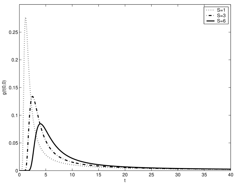
Figure 1: Evaluation of the FPT probability density function for an IBM through three different boundaries: $S=1$ (dotted), $S=3$ (dashdot), $S=6$ (solid).

5.2 Integrated Ornstein Uhlenbeck Process

As the IBM, the IOU Process is not a Markov process and it should be studied as a bivariate process together with an Ornstein Uhlenbeck Process, as follows

$$\left\{\begin{array}[]{lll}dX_{1}(t)&=&X_{2}(t)dt\\ \\ dX_{2}(t)&=&\left(-\alpha X_{2}(t)+\mu\right)dt+\sigma dB_{t},\end{array}\right.$$ (33)

with $\mathbf{X}(0)=\mathbf{0}$. The process (33) is a Gauss-Markov process (8), where

$$\mathbf{A}(t)=\left(\begin{array}[]{cc}0&1\\ 0&-\alpha\end{array}\right)\mbox{, }\mathbf{M}(t)=\left(\begin{array}[]{ll}0\\ \mu\end{array}\right)\mbox{ and }\mathbf{G}(t)=\left(\begin{array}[]{cc}0&0\\ 0&\sigma\end{array}\right)\mbox{.}$$

Note that in this case the constant $C$ defined in Remark 2 is equal to 1 and the range of the random variable $X_{2}(T)$ is $[-\infty,\infty]$.

In Figure 2 we show the FPT probability density function of the IOU through a boundary $S=6$, for $\mu=0.01$, $\sigma=1$ and three different values of the parameter $\alpha$.

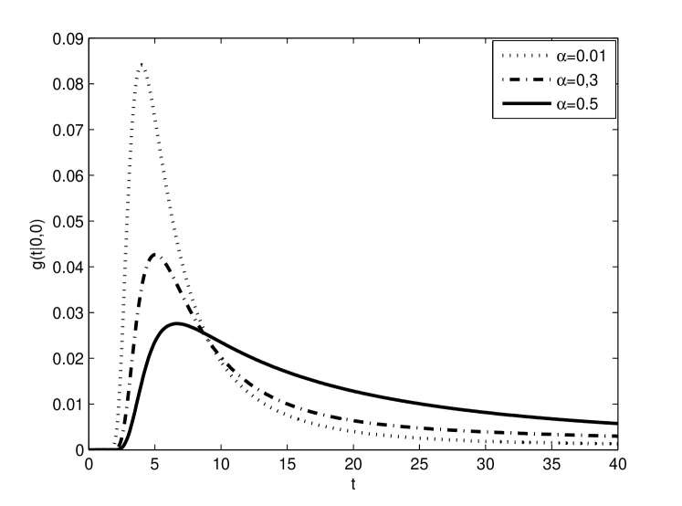
Figure 2: Evaluation of the FPT probability density function of the IOU through a boundary $S=6$ for $\mu=0.01$, $\sigma=1$ and three different values of the parameter $\alpha$: $\alpha=0.01$ (dotted), $\alpha=0.3$ (dashdot), and $\alpha=0.5$ (solid).

Note that the curve for $\alpha=0.01$ in Figure 2 is very similar to the curve for $S=6$ in Figure 1, indeed if $\mu\rightarrow 0$ and $\alpha\rightarrow 0$ IOU converges to a standard IBM.

5.3 Two-compartment model

One dimensional neuronal models [21] identify the membrane potential values on the different parts of the neuron with those assumed in the trigger zone. To improve the model [15] proposes a two dimensional approach. The membrane potential of a neuron is described by means of a bivariate stochastic process, whose components represent the depolarizations of two distinct parts, the trigger zone and the dentritic one.

Let $(X_{1}(t))_{t\geq 0}$ and $(X_{2}(t))_{t\geq 0}$ be the stochastic processes associated to the depolarization of the trigger zone and the dendritic one, respectively. Then, assuming that external inputs, of intensity $\mu$ and variability $\sigma$, influence only the second compartment and taking the interconnection between the parts into account, we obtain the following stochastic model

$$\left\{\begin{array}[]{lll}dX_{1}(t)=\left\{-\alpha X_{1}(t)+\alpha_{r}\left[X_{2}(t)-X_{1}(t)\right]\right\}dt\\ \vspace{0.1mm}\\ dX_{2}(t)=\left\{-\alpha X_{2}(t)+\alpha_{r}\left[X_{1}(t)-X_{2}(t)\right]+\mu\right\}dt+\sigma dB_{t}\end{array}\right.$$ (34)

with $\mathbf{X}(0)=\mathbf{0}$ and where $\alpha$ and $\alpha_{r}$ are constant related to the spontaneous membrane potential decay and to the intensity of the connection between the two compartments, respectively (cf. Fig 3).

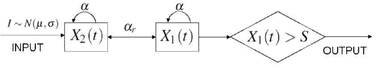
Figure 3: Schematic representation of the two-compartment approach

The process (34) is an Ornstein Uhlenbeck two-dimensional process, particular case of the Gauss-Markov process (8) where

$$\mathbf{A}(t)=\left(\begin{array}[]{cc}-\alpha-\alpha_{r}&\alpha_{r}\\ \alpha_{r}&-\alpha-\alpha_{r}\end{array}\right)\mbox{, }\mathbf{M}(t)=\left(\begin{array}[]{ll}0\\ \mu\end{array}\right)\mbox{ and }\mathbf{G}(t)=\left(\begin{array}[]{cc}0&0\\ 0&\sigma\end{array}\right)\mbox{.}$$

Note that in this case the constant $C$ defined in Remark 2 is equal to 2 and the range of the random variable $X_{2}(T)$ is $[kS,\infty]$, where

$$k=\frac{\alpha+\alpha_{r}}{\alpha_{r}}.$$

Assuming that after each spike the system is reset to its initial value, the time between two spikes, i.e. the time when the membrane potential changes its dynamics with a sudden hyperpolarization, is described by the FPT of the first component through a boundary $S$.
In [15] this model was studied using simulation techniques, but applying the algorithm proposed in Section 4 we can compute the interspike intervals distribution as the FPT probability density function of the first component of $\mathbf{X}(t)$. In Figure 4 we show the FPT density for a set of values of the input.

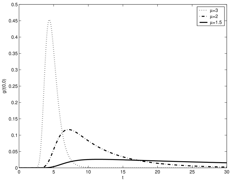
Figure 4: Evaluation of the FPT probability density function through a boundary $S=6$ for a two-compartment stochastic model of a neuron, choosing $\alpha=0.33$, $\alpha_{r}=0.2$, $\sigma=1$ and three different values of $\mu$: $\mu=1.5$ (solid), $\mu=2$ (dashdot), and $\mu=3$ (dotted).

6 Numerical algorithm versus a totally simulation algorithm

The introduced numerical method involves a Monte Carlo estimation to evaluate the expected value (24). One may wonder about the advantages of the proposed method with respect to a totally simulation algorithm. Indeed it is easy to simulate $M$ sample paths of the considered bivariate process to get a sample of FPTs. These FPTs could be used to draw histograms or their continuous approximations. However this approach is computationally expensive. Indeed it requires large samples to give reliable results. Moreover the estimation of the tails of the distribution is scarcely reliable and time consuming.

On the contrary the numerical method proposed here requests weak computational efforts despite the presence of the Monte Carlo method and is applied to estimate a specific integral, i.e. the expectation (24). Indeed, also a small number of trajectories guarantees reliable results.

In Figure 5 we compare the accuracy of the results obtained with the two methods. We simulate $M$ sample paths of the IBM in order to determine a sample of $M$ FPTs and we use it to draw the corresponding histogram. The same sample is used to compute the sample mean (25) to get the FPT probability density function via the numerical method. The choice $M=1000$ gives reliable results in both cases. However, when $M=50$ the histogram is rude while the numerical method does not loose its reliability. We further underline how the computational time to build the histogram or to draw the FPT density with the proposed numerical method are comparable, for the same value of $M$.

In Figure 6 we show the shapes of the FPT probability density function obtained via the proposed numerical algorithm. We use a sample of size $M=50$ (solid line) and $M=1000$ (dash line) to compute (25). Their differences are negligible.

(a) $M=50$

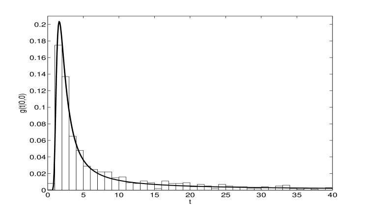
(b) $M=1000$

Figure 5: FPT probability density function for the IBM obtained via the proposed numerical method and the corresponding histogram. Sample of size $M$ has been used to build the histogram and to evaluate (25) in the numerical method: (a) $M=50$ (b) $M=1000$.

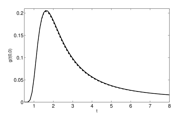
Figure 6: FPT probability density function for the IBM obtained via the proposed numerical method computed using a sample of size $M=50$ (solid line) and $M=1000$ (dash line) for the sample mean (25).

7 Conclusion

We studied the FPT of one component of a bivariate diffusion process through a boundary. We wrote a new integral equation for the FPT probability density function proving its existence and uniqueness. A numerical algorithm for its solution was developed proving its convergence properties. The algorithm was applied to a set of processes of interest for various applications. Advantages of the method with respect to a totally simulation algorithm are discussed.

The crossing problem for one component of a multivariate process or the case of random initial value can be treated as extensions of the proposed equations and of the numerical algorithm.

8 Acknowledgements

Work supported in part by MIUR Project PRIN-Cofin 2008.

References

• [1] Abramowitz M. and Stegun I. A., Handbook of Mathematical Functions With Formulas, Graphs, and Mathematical Tables. Dover, New York (1964).
• [2] Arnold L., Stochastic differential equations: theory and applications. Krieger publishing company, Malabar, Florida (1974)
• [3] Buonocore, A., Nobile, A.G. and Ricciardi, L.M., A new integral equation for the evaluation of first-passage-time probability densities. Adv. in Appl. Probab. 19 4, 784-800 (1987)
• [4] Di Nardo E., Nobile A.. Pirozzi E. and Ricciardi L.M., A computational approach to first-passage-time problems for Gauss-Markov processes, Adv. Appl. Prob. 33, 453–482 (2001)
• [5] Downes A. N. and Borovk K., First Passage Densities and Boundary Crossing Probabilities for Diffusion Processes, Methodology and Computing in Applied Probability, Volume 10, Number 4, 621–644 (2008)
• [6] Durbin J., The first passage density of a continuous Gaussian process to a general boundary, J.Appl. Prob. 22, 99–122 (1985)
• [7] Durbin J., The first passage density of the Brownian motion process to a curved boundary, J. Appl. Prob. 29, 291–304 (1992)
• [8] Giorno V., Nobile A.G. and Ricciardi L.M., A symmetry-based constructive approach to probability densities for one-dimensional diffusion processes, J. Appl. Prob. 27, 707–721 (1989)
• [9] Giorno V., Nobile A.G. and Ricciardi L.M., On the asymptotic behavior of first-passage-time densities for one dimensional diffusion processes and varying boundary, Adv. Appl. Prob. 22, 883–914 (1990)
• [10] Giorno V., Nobile A.G., Ricciardi L.M. and Di Crescenzo A., On a symmetry-based constructive approach to probability densities for two-dimensional diffusion processes, J. Appl. Prob. 32, 316–336 (1995)
• [11] Giraudo M.T. and Sacerdote L., An improved technique for the simulation of first passage times for diffusion processes, Communication in Statistics: simulation and computation, 28, n.4, 1135–1163 (1999)
• [12] Giraudo M.T., Sacerdote L. and Zucca C., Evaluation of first passage times of diffusion processes through boundaries by means of a totally simulative algorithm, Meth. Comp. Appl. Prob. 3, 215–231 (2001)
• [13] Goldman M., On the First Passage of the Integrated Wiener Process, The Annals of Mathematical Statistics, Vol. 42, No. 6, 2150–2155 (1971)
• [14] Lachal A., On the first passage time for integrated Brownian motion (in French), Ann. I. H. P., Sect. B 27(3), 385–405 (1991)
• [15] Lansky P. and Rodriguez R., Two-compartment stochastic model of a neuron, Physica D 132, 267–286 (1999)
• [16] Linz P., Analytical and numerical methods for Volterra equations. SIAM, Philadelphia (1985)
• [17] Nobile A.G., Ricciardi L.M. and Sacerdote L., Exponential trends of first passage time densities for a class of diffusion processes with steady-state distribution, J. Appl. Prob. 22, 611–618 (1985)
• [18] Panfilo G., Tavella P and Zucca C., Stochastic Processes for modelling and evaluating atomic clock behaviour, Advanced Mathematical and Computational Tools in Metrology VI, P. Ciarlini,M. G. Cox,F. Pavese ed. World Scientific Publishing (2004)
• [19] Peskir G., Limit at zero of the Brownian first-passage density. Probab. Theory Related Fields. 124, 100-111 (2002)
• [20] Redner S., A guide to first-passage processes. Cambridge University Press (2001)
• [21] Ricciardi L.M., Lecture Notes in Biomathematics. Springer Verlag, Berlin (1977)
• [22] Ricciardi L.M., Sacerdote L. and Sato S., On an Integral Equation for First-Passage-Time Probability Densities, Journal of Applied Probability, Vol. 21, No. 2, 302–314 (1984)
• [23] Ricciardi, L.M. and Sato, S., Diffusion processes and first-passage-time problems. In: L.M. Ricciardi (Ed.), Lectures in Applied Mathematics and Informatics. Manchester Univ. Press., Manchester (1990)
• [24] Román P., J.J. Serranoa J.J. and Torres F., First-passage-time location function: Application to determine first-passage-time densities in diffusion processes, Computational Statistics & Data Analysis, Volume 52, Issue 8, 4132–4146 (2008)
• [25] Sacchetto L., Tempo di primo passaggio del moto browniano integrato: aspetti analitici, numerici e simulativi. Tesi di laurea specialistica in matematica, Università di Torino (2009)
• [26] Sacerdote L., Asymptotic behavior of Ornstein-Uhlenbeck first-passage-time density through boundaries, Applied Stochastic Models and Data Analysis. 6, 53–57 (1988)
• [27] Sacerdote L. and Giraudo M.T., Stochastic integrate and fire models: a review on mathematical methods and their applications. To appear in Lecture Notes in Mathematics, Series Mathematical biosciences (2010)
• [28] Sacerdote L. and Tomassetti F., On Evaluations and Asymptotic Approximations of First-Passage-Time Probabilities, Advances in Applied Probability, Vol. 28, No. 1, 270–284 (1996)
• [29] Smith P.L., From Poisson shot noise to the integrated Ornstein Uhlenbeck process: Neurally principled models of information accumulation in decision-making and response time, Journal of Mathematical Psychology 54, 266–283(2010)
• [30] Wang L. and Pötzelberger K., Crossing Probabilities for Diffusion Processes with Piecewise Continuous Boundaries, K. Methodology and Computing in Applied Probability, Volume 9, Number 1, 21–40 (2007)