Extreme events in two dimensional disordered nonlinear lattices

Abstract

Spatiotemporal complexity is induced in a two dimensional nonlinear disordered lattice through the modulational instability of an initially weakly perturbed excitation. In the course of evolution we observe the formation of transient as well as persistent localized structures, some of which have extreme magnitude. We analyze the statistics of occurrence of these extreme collective events and find that the appearance of transient extreme events is more likely in the weakly nonlinear regime. We observe a transition in the extreme events recurrence time probability from exponential, in the nonlinearity dominated regime, to power law for the disordered one.

Nonlinear lattices form a unique laboratory where both coherent and incoherent processes appear simultaneously and affect their dynamical properties Flach . They constitute prototypical spatiotemporally complex systems that can be studied both theoretically and experimentally giving a wealth of information on the physics of spatially extended complex systems. The additional presence of quenched disorder introduces a mechanism for local symmetry breaking that has consequences in the long-time dynamics disorder . One feature of selforganization of the lattices relates to the possibility for occurrence of extreme events (EE), i.e. the generation of transient or persistent structures with large amplitudes that are statistically not very significant. In the case of ocean waves, events of this type are rogue or freak waves, i.e. waves of considerable hight that ”appear from nowhere and disappear without a trace” Akhmediev2009a , usually in relatively calm seas Albeverio2006 ; Kharif2009Debate2010 . Ocean rogue waves are attributed to self-focusing effects following the development of Benjamin-Feir instabilityWhite1998 . Extreme waves of this type have also been reported in nonlinear optical fibers Solli2007 ; Arecchi2011 , optical cavities Montina2009 , superfluids Ganshin2009 , microwave scattering Hohmann2010 , semiconductor lasers Bonatto2011 , femtosecond filamentation Majus2011 , soft glass photonic crystal fiber Buccoliero2011 , etc.

In the present work we focus on two dimensional discrete nonlinear systems with disorder that have been realized experimentally Schwartz2007 and address the question of the conditions for generation of very large, i.e. extreme, discrete wave events in the process of spatiotemporal evolution. While the production of EEs is mediated by modulational instability (MI) the subsequent evolution shows a complex dynamics that leads to generation as well as destruction of waves of large magnitude. This dynamics is directly induced by the interplay of nonlinearity and disorder; we are seeking the regimes where EE appearance is the most frequent as well the statistics of their appearance. In recent work we found that integrability properties of the lattice do play a role in the generation of EEs Maluckov2009 . The present work, focusses on the issue of discrete lattice EEs from a broader perspective and through a physically realizable model, viz. that of the Anderson disordered Discrete Nonlinear Schrödinger (DNLS) equation Schwartz2007 ; Lahini2008 . We address two experimentally relevant questions, viz. what is the optimal regime for EE generation and what is the recurrence time statistics of these events once generated. From this analysis a clearer picture of the spatiotemporal complexity of the system emerges.

We consider the dynamics of a strongly coupled excitation in a two dimensional tetragonal lattice with diagonal disorder, or, equivalently, wave propagation in a two dimensional array of evanescently coupled optical nonlinear fibers with random index variation, both described through the disordered DNLS equation, viz.

$$i\frac{d{\psi}_{n,m}}{dt}={\epsilon}_{n,m}{\psi}_{n,m}+J({\psi}_{n+1,m}+{\psi}_{n-1,m}+{\psi}_{n,m+1}+{\psi}_{n,m-1})+\gamma\left|{\psi}_{n,m}\right|^{2}{\psi}_{n,m},$$ (1)

where $n,m=1,...,N$, $\psi_{n,m}$ is a probability (or wave) amplitude at site $(n,m)$ , $J>0$ is the inter-site coupling constant accounting for tunnelling between adjacent sites of the lattice (corr. evanescent coupling), $\gamma>0$ is the nonlinearity parameter that stems from strong electron-phonon coupling (corr. Kerr nonlinearity), while ${\epsilon}_{n,m}$, is the local site energy (related to the fiber refractive index), chosen randomly from a uniform, zero-mean distribution in the interval $[-W/2,+W/2]$. Equation (1) serves as a paradigmatic model for a wide class of physical problems where both disorder and nonlinearity are present. For $\gamma\rightarrow 0$, Eq.(1) reduces to the 2D Anderson model while in the absence of disorder (${\epsilon}_{n,m}=0$), it reduces to the DNLS equation in 2D that is generally non-integrable. Equation (1) conserves the norm $P_{N}=\sum_{n=1}^{N}\sum_{m=1}^{M}|{\psi}_{n,m}|^{2}$, and the Hamiltonian $\cal{H}$, corresponding to total probability (corr. input power) and the energy of the system, respectively. We will consider the evolution of an initially uniform state that is slightly modulated by periodic perturbations in order to facilitate the development of MI Kivshar1994 , Wollert2009 . Specifically, we use the initial state ${\psi}_{n,m}=({\psi}_{0}+\delta{\psi}_{n,m})\exp({-i\mu t})$, where ${\psi}_{0}$ is a constant amplitude of the continuous wave (CW) (averaged over disorder, with $\langle\epsilon_{n,m}\rangle=0$), and $\delta{\psi}_{n,m}\equiv a_{n,m}+ib_{n,m}$ are small complex perturbations that modulate the constant CW solution. The MI induces nonlinearly localized modes that are, however, modified by the presence of the quenched disorder. In the time scale of the numerical study, we note that the presence of disorder induces some form of additional energy redistribution among the sites of nonlinear lattice.

We adopt the criterion employed in oceanography and define as an extreme wave one that has height $H_{ext}$ (here the positive difference of minimum-to-maximum amplitude $|\psi_{n,m}|$ in different time steps) with $H_{ext}\gtrsim 2.2H_{s}$, where $H_{s}$, is the significant wave height, i.e. average height of the one-third highest waves in a given sample Kharif2009Debate2010 . We integrate Eqs. (1) with periodic boundary conditions using a $6-$th order Runge-Kutta Maluckov2009 solver for several different values of $W$ and $\gamma$ ($J=1$) using typically a lattice with $N=41$ (we have checked results for $N=81$ as well) and periodic boundary conditions. During relatively long time (typically we used maximum time of $1\times 10^{3}$ units or equivalently approximately $500$ coupling lengths) the system selforganizes and we observe localized structures appearing on different sites surrounded by irregular, low-amplitude background. Some of these structures are in the form of breathers, either pinned or mobile, while some others are transient. The complete amplitude statistics for the observed time interval is shown in Fig. (1a) for different disorder and nonlinearity parameters; we observe a distinct, Rayleigh-like distribution that vary depending on the parameters. Any of the states, longer lived or transient, that appear in tail of the distribution are candidates for extreme events.

In order to quantify the onset of extreme events in the lattice we use several measures, viz. the inverse participation ratio, the probability for extreme event occurrence as well as first appearance and recurrence EE times. The inverse participation ratio

$$P={P_{N}^{2}}\left\{\sum_{n=1}^{N}\sum_{m=1}^{M}|f_{n,m}|^{4}\right\}^{-1},$$ (2)

determines the effective confinement of initially extended excitations. We define $\omega_{eff}=P^{1/2}$; this effective width gives the average spatial extent of the structures generated after the MI (Fig. (1b)).

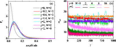
Figure 1: (color online) Probability amplitude distribution $P_{s}$ as a function of amplitude $|\psi|$ for different nonlinearity strengths and $W=2$ (a). The curves have a Rayleigh-like behavior. (b) Effective average width of excitations formed in the lattice as a function of time for different disorder levels for $\gamma=0,~{}2$. We note that for fixed nonlinearity, increase in the amount of disorder induces delocalization.

Both disorder and nonlinearity, when each acts alone, favor wave localization in the lattice. When they are present simultaneously, quenched disorder dominates the early dynamics since MI develops more slowly, at least for relatively small $\gamma$’s. In this regime, where both nonlinearity and disorder are present, the Anderson-like localized states decay spatially in a fashion that still permits local energy redistribution, while at relatively longer times a more stable state is reached. We note from Fig. (1b) that $\omega_{eff}$ saturates to lower values for non-zero nonlinearity compared to the value in the corresponding linear disordered system. This tendency is compatible with the findings of Schwartz et al. who observe experimentally that increased self-focusing enhances localization Schwartz2007 . On the other hand, we also see in the same figure that increasing disorder for fixed nonlinearity results to larger $\omega_{eff}$, leading thus to reduction of localization. This opposite tendency of delocalization induced by disorder in the presence of nonlinearity can be attributed to the partial destruction of the pinned, highly localized nonlinear states by the presence of disorder and the associated weak redistribution of energy.

In order to find the regimes that favor EE production we calculate numerically $P_{ee}$, the probability for EE generation with $h>H_{ext}\equiv 2.2H_{s}$; it is shown in Fig. 2 as a function of $\gamma$ for three different levels of disorder. From Fig. 2 we observe that increasing the strength of nonlinearity results in an increase in the EE probability $P_{ee}$, reaching generally a maximum, while at high nonlinearity parameter values ( $\gamma>2$ ), the EE probability reduces for all observed disorder levels. We note that for small disorder the curve has additionally a secondary maximum while the occurrence of the primary maximum value shifts to large $\gamma$-values for larger amounts of disorder $W$. Further increase of nonlinearity leads to the decay of the extreme event generation probability, however, with a tail that is substantially higher for the larger disorder case. For vanishingly small nonlinearity, $P_{ee}$ is small but with appreciable values; we find $P_{ee}=0.47,~{}0.44$ for disorder levels with $W=2,~{}4$, respectively. These results indicate that the most favorable conditions for the EE generation during propagation through in the 2D lattice systems are relatively high level of disorder compared to the linearized bandwidth and presence of nonlinearity. The interplay of disorder and nonlinearity results in one or more maxima in the probability of EE generation for certain values of the nonlinearity strength. The first maximum which is the most pronounced one for relatively small disorder and weak nonlinearity can be correlated with high EEs probability in the near integrable system pointed out in the 1D context Maluckov2009 . On the other hand, for arbitrary disorder the localizing effect of nonlinearity seems to be responsible for the appearance of the second maximum at $\gamma\approx 2$ with a value $P_{ee}\approx 0.7\%$.

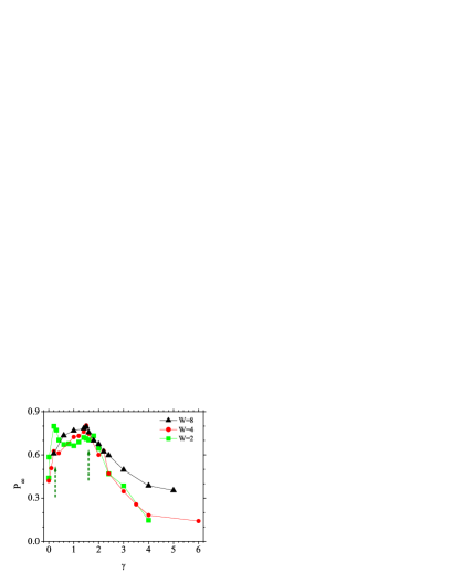
Figure 2: (color online) Extreme event height probability $P_{ee}$ as a function of the nonlinearity strength $\gamma$ for several levels of disorder. Arrows show positions of local probability maximums.

In order to probe deeper into the genesis and appearance statistics of EEs in discrete, disordered nonlinear lattices we focus on the probability distribution $P_{r}$ of the recurrence time $r$ of the extreme events Altmann2005 , Santhanam2008 . We study two quantities, the mean recurrence time $R$ of an EE as well as the mean time of first appearance (TFA). As these times depend on the specific value of the parameter $q$, the wave height threshold, we first investigate their dependence on $q$. Numerics show that the slope of the curves of the recurrence time $R$ as a function of the threshold $q$ is smaller when only disorder is present compared to the case of simultaneous presence of disorder and nonlinearity for all levels of disorder (Fig. 3a). The mean recurrence time $R$ increases with $q$ for all values of $W$ and $\gamma$ (Fig. 3). The increase is faster for lower disorder level (Fig. 3a) and stronger nonlinearity (Fig. 3b). This dependence in the strong nonlinearity-weak disorder regime is related to the favorable conditions for the creation of highly pinned, immobile localized structures, a fact that increases dramatically the mean recurrence time. Qualitatively similar behavior we found also for the TFA-$q$ dependence. These studies show the complexity of the recurrence as well as first appearance phenomena and their direct manifestation in time average quantities.

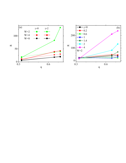
Figure 3: (color online) The average return time $R$ of extreme events as a function of the threshold amplitude $q$ for (a) various disorder levels with $\gamma=0$ (circles) and $\gamma=2$, (b) fixed level of disorder ($W=2$) and several nonlinearity strengths (including zero nonlinearity).

We calculate $P_{r}$, the return time probability for different disorder levels and nonlinearity values in the following way. For a given threshold value $q$ ($q>H_{ext}$) we scan the lattice and find an event at a given location with amplitude larger than $q$; we register as recurrence time the time between this event and a subsequent above threshold one that appears in the same lattice location . We follow this procedure repeatedly up to maximum time and construct histograms for different parameter values, all scaled by the average return time $R$ in each parameter regime; the outcomes for the various non normalized return probabilities are shown in Fig. 4 for several values of disorder level and nonlinearity for a given $q$-value. In the purely linear but disordered regime we find that $P_{r}$ is a power-law function, viz. $P_{r}=[a+b(r/R)]^{-\beta}$, with $\beta\approx 1.34$ $q=0.66$; while the parameters depend on the threshold value $q$, the functional form is stable. The addition of nonlinearity to a disordered lattice reduces somehow the possibility of occurrence of EEs. Remarkably, the $P_{r}$ vs. $r/R$ dependence of the curves changes gradually from power-law, in the linear, disordered regime, to a double exponential at intermediate nonlinearity values to single exponential for a pure nonlinear lattice with no or very little disorder. Furthermore, the decay of the curves is more rapid for higher nonlinearity strength. The observed transition from a power law, in the disordered dominated regime, to exponential, in the nonlinearity dominated one, is linked to the behavior of the tail of the amplitude probability distributions.

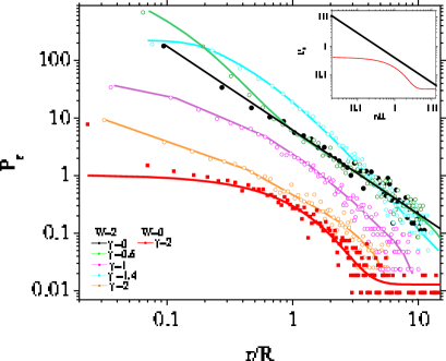
Figure 4: (color online) Return time probability $P_{r}$ (not normalized) as a function of $r/R$, the return time scaled by the corresponding average return time, for the purely disordered case (power law fit - black curve), purely nonlinear case (exponential fit - red line) and intermediate cases (double exponential fits). We use $q=0.66$. In box the lines which designate the first two cases are shown separately.

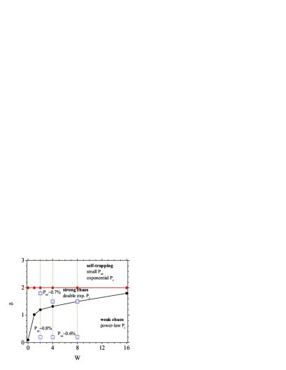
Figure 5: (color online) Different regimes of the spreading of wave-packets in the effective parameter space $(W,\delta)$  Flach1d ; Flach2d . Lines represent regime boundaries $\delta\approx d$ and $\delta=2$. Empty squares denote parameters for which the local maximums of $P_{ee}$ are found (2).

We relate our relatively short-time results to expected long-time wave-packet spreading regimes summarized in Ref. Flach1d and Flach2d (one-dimensional DNLS with disorder and its generalization to the higher dimensional problem, respectively). Different regimes are obtained for (i) $\delta>2$, onset of selftrapping, (ii) $d<\delta<2$, strong chaos and (iii) $\delta<d$ for the effective quantities $d$ and $\delta$. The latter are the average frequency spacing of the nonlinear modes within a localization volume given by $d\approx\Delta/V=(8J+W)/\omega_{eff}$ while the nonlinear frequency shift $\delta$ is taken to be $\delta\approx\gamma$. The selection of regimes in Flach1d ; Flach2d was done taking into account the intensity of interaction among the nonlinear modes; the latter increases with the nonlinearity strength up to the high nonlinearity (here $\delta\approx 2$) when the strong self-trapping results in a creation of isolated strongly pinned high amplitude breathers. The comparison is approximate but leads to interesting observations (see Fig. 5). The first local maximum in the $P_{ee}$ found for small nonlinearity strength is located in the weak chaos regime. Its maximal value $P_{ee}\approx 0.8\%$ is observed for small $W$. The second, broader maximum of $P_{ee}$ for all disorder cases is located in the strong chaos regime relatively close to the border lines with neighboring regimes (Fig. 5). On the other hand, we may associate the power-law decay of the $P_{r}$ to the weak chaos regime, and the exponentially like one with the self-trapping regime. Therefore, transient EEs are more probable in the regime of weak chaos, while the long-lived EEs (high amplitude strongly pinned breather structures) are dominant structures in the regimes of strong chaos and self-trapping. This association enables us to relate the first local maximum in $P_{ee}$ to the weak interaction of transient EEs induced by disorder while the second, broader maximum, to the appearance of longer-lived breathers resulting from the energy redistribution through the strong interaction between nonlinear modes.

We have calculated several statistical measures for wave propagation in disordered and nonlinear lattices described by the DNLS in two-dimensions with respect to EEs generation. The interplay of two distinct mechanisms of energy localization leads to several unexpected results. The calculations indicate that EEs may be generated with appreciable probability also in linear disordered lattices (but not in linear non-disordered lattices) for the chosen type of initial excitations.

When the relative strengths of nonlinearity and disorder vary, the average return probability $P_{r}$ of EEs as a function of $r/R$ changes between the two limiting regimes, i.e., disorder without nonlinearity and nonlinearity without disorder corresponding respectively to a transition from power-law to exponential . These findings are illustrated in Fig. 4 for certain parameter values. The change occurs gradually between the two regimes passing through a sequence of states that have more complex return time behavior. Moreover, the calculated probability for EE generation indicates that there are two parameter regimes of the disorder level and nonlinearity strength which favor EE generation, as shown in Fig. (2). We found that a relatively low level of disorder (compared to the bandwidth) leads to maxima in the probability for EE production in the relatively weak nonlinearity regime. The second, broader, maximum found for higher nonlinearity does not depend significantly on the disorder level. For very high $\gamma$’s the probability of EE generation, although small, depends strongly on the level of the disorder. The fact that EE generation is favorable in the weakly nonlinear regime appears to be compatible with previous findings in discrete lattices, where the highest probability for EE generation is observed in the nearly integrable limit Maluckov2009 . On the other hand, the appearance of the second parameter regime which favors the EE generation is correlated with the localization mechanism governed by nonlinearity Molina1993 . We also note that the mechanism responsible for the probability for EE generation depends additionally on the specific initial conditions used, as seen also in other approaches Bludov2009 .

- (1) S. Flach and A. V. Gorbach, Phys. Rep. 467, 1 (2008), and references therein.
- (2) M. I. Molina et al., Phys. Rev. Lett. 73, 464 (1994) , M. I. Molina, Phys. Rev. B 58, 12547 (1998), G. Kopidakis et al.,Phys. Rev. Lett. 84, 3236 (2000), G. Kopidakis et al., Phys. Rev. Lett. 100, 084103 (2008). S. Flach et al., Phys. Rev. Lett. 102, 024101 (2009). A. S. Pikovsky et al., Phys. Rev. Lett. 100, 094101 (2008).
- (3) N. Akhmediev, A. Ankiewicz, and M. Taki, Phys. Lett. A 373, 675 (2009);
- (4) S. Albeverio, V. Jentsch, H. Kantz (Eds.), Extreme events in nature and society, (Springer-Verlag, Berlin, 2006).
- (5) C. Kharif, E. Pelinovsky, and A. Slunyaev, Rogue Waves in the Ocean, (Springer-Verlag, Berlin, 2009); N. Akhmediev and E. Pelinovsky, (Eds.) Special Issue: Discussion Debate: Rogue Waves - Towards a Unifying Concept?, Eur. Phys. J. Spec. Top. 185, (2010).
- (6) B. S. White and B. Forneberg, J. Fluid Mech. 355, 113 (1998).
- (7) D. R. Solli, et al., Nature 450, 1054 (2007;
- (8) F. T. Arecchi et al., Phys. Rev. Lett. 106, 153901 (2011).
- (9) A. Montina et al., Phys. Rev. Lett. 103, 173901 (2009).
- (10) A. N. Ganshin et al., J. Phys.: Conf. Series 150, 032056 (2009).
- (11) R. Höhman et al., Phys. Rev. Lett. 104, 093901 (2010).
- (12) C. Bonatto et al., Phys. Rev. Lett. 107, 053901 (2011).
- (13) D. Majus et al., Phys. Rev. A 83, 025802 (2011).
- (14) D. Buccoliero et al., Opt. Express 19, 17973 (2011).
- (15) T. Schwartz, et al., Nature 446, 05623 (2007).
- (16) A. Maluckov, et al., Phys. Rev. E 79, 025601(R) (2009).
- (17) Y. Lahini et al., Phys. Rev. Lett. 100, 013906 (2008).
- (18) Yu. S. Kivshar and M. Salerno, Phys. Rev. E 49, 3543 (1994).
- (19) A. Wöllert et al., Acta Phys. Pol. A 116, 519 (2009).
- (20) E. G. Altmann and H. Kantz, Phys. Rev. E 71, 056106 (2005);
- (21) M. S. Santhanam and H. Kantz, Phys. Rev. E 78, 051113 (2008).
- (22) T. V. Laptyeva, J. D. Bodyfelt, D. O. Krimer, Ch. Skokos and S. Flach, EPL, 91, 30001 (2010).
- (23) S. Flach, Chemical Physics 375, 548 (2010).
- (24) M. I. Molina and G. P. Tsironis, Physica D, 65, 267 (1993).
- (25) Yu. V. Bludov, et al., Opt. Lett. 34, 3015 (2009).