Boolean nested canalizing functions: a comprehensive analysis

Abstract.

Boolean network models of molecular regulatory networks have been used successfully in computational systems biology. The Boolean functions that appear in published models tend to have special properties, in particular the property of being nested canalizing, a concept inspired by the concept of canalization in evolutionary biology. It has been shown that networks comprised of nested canalizing functions have dynamic properties that make them suitable for modeling molecular regulatory networks, namely a small number of (large) attractors, as well as relatively short limit cycles.

This paper contains a detailed analysis of this class of functions, based on a novel normal form as polynomial functions over the Boolean field. The concept of layer is introduced that stratifies variables into different classes depending on their level of dominance. Using this layer concept a closed form formula is derived for the number of nested canalizing functions with a given number of variables. Additional metrics considered include Hamming weight, the activity number of any variable, and the average sensitivity of the function. It is also shown that the average sensitivity of any nested canalizing function is between 0 and 2. This provides a rationale for why nested canalizing functions are stable, since a random Boolean function in $n$ variables has average sensitivity $\frac{n}{2}$. The paper also contains experimental evidence that the layer number is an important factor in network stability.

1. Introduction

Canalizing Boolean functions were introduced by S. Kauffman and collaborators [20] as appropriate rules in Boolean network models of gene regulatory networks. More recently, a subclass of these functions, so-called nested canalizing functions (NCF) was introduced [21] and studied from the point of view of stability properties of network dynamics. A multi-state version of such functions has been introduced in [33, 34], where it was shown that networks whose dynamics are controlled by nested canalizing functions have similar stability properties, namely large attractor basins and short limit cycles. An analysis of published models, both Boolean and multi-state, of molecular regulatory networks revealed that the large majority of regulatory rules in them is canalizing, with most of these in fact nested canalizing [14, 22, 35, 33]. Thus, nested canalizing rules and the properties of networks governed by them are important to study because of their relevance in systems biology. Furthermore, they are also important in computational science. In [16] it was shown that the class of nested canalizing Boolean functions is identical to the class of so-called unate cascade Boolean functions, which has been studied extensively in engineering and computer science. It was shown, for instance, in [8] that this class has the property that it corresponds exactly to the class of Boolean functions with corresponding binary decision diagrams of shortest average path length. Thus, a more detailed mathematical study of nested canalizing functions might have applications to problems in engineering as well.

In this paper, we carry out such a detailed study for the case of Boolean nested canalizing functions, obtaining a more explicit characterization than the one obtained in [17]. We introduce a new concept, the layer number, leading to a finer classification and, in particular, an explicit formula for the number of nested canalizing functions. This provides a closed form solution to the recursive formula derived in [17], which may be of independent mathematical interest. We also study standard properties of Boolean functions, such as variable activity and average sensitivity. In particular, we obtain a formula for the average sensitivity of a nested canalizing function with $n$ variables, and show that, for all $n$, it lies between $\frac{n}{2^{n-1}}$ as a lower bound and $2$ as upper bound, which is much smaller than $\frac{n}{2}$, the average sensitivity of a random Boolean function in $n$ variables. This can be interpreted as providing a theoretical justification for why Boolean networks with nested canalizing rules are stable. We also find a formula for the Hamming weight (the number of 1’s in its truth table) of a nested canalizing function. Finally, we conjecture that a nested canalizing function with $n$ variables has maximal average sensitivity if it has the maximal layer number $n-1$. Based on this result, we conjecture the tight upper bound $\frac{4}{3}$ for this value. The paper is organized as follows. We first review existing results on nested canalizing functions and networks, after which we introduce some definitions and notation. The subsequent sections contain the main results of the paper.

2. Background

In [32] it was shown that the dynamics of a Boolean network which operates according to canalizing rules is robust with regard to small perturbations. In [19], an exact formula was derived for the number of Boolean canalizing functions. In [30], the definition of canalizing functions was generalized to any finite field $\mathbb{F}_{q}$, where $q$ is a power of a prime. Both exact formulas and asymptotic values for the number of generalized canalizing functions were obtained.

One important characteristic of (nested) canalizing functions is that they exhibit a stabilizing effect on the dynamics of a Boolean network. That is, small perturbations of an initial state do not grow larger over time and eventually end up in the same attractor as the initial state. This stability is typically measured using so-called Derrida plots which monitor the Hamming distance between a random initial state and its perturbed state as both evolve over time. If the Hamming distance decreases over time, the system is considered stable. The slope of the Derrida curve is used as a numerical measure of stability. Roughly speaking, the phase space of a stable system has few components and the limit cycle of each component is short.

In [22], the authors studied the dynamics of nested canalizing Boolean networks over a variety of dependency graphs. That is, for a given random graph on $n$ nodes, where the in-degree of each node is chosen at random between $0$ and $k$, for $k\leq n$, a nested canalizing function is assigned to each node in the in-degree variables of that node. The dynamics of these networks was then analyzed and the stability measured using Derrida plots. It was shown there that nested canalizing networks are remarkably stable regardless of the in-degree distribution and that the stability increases as the average number of inputs of each node increases.

Most published molecular networks are given in the form of a wiring diagram, or dependency graph, constructed from experiments and prior published knowledge. However, for most of the molecular species in the network, little knowledge, if any, could be deduced about their regulatory rules, for instance in the gene transcription networks in yeast [15] and E. Coli [3]. Each one of these networks contains more than 1000 genes. Kauffman et. al [21] investigated the effect of the topology of a sub-network of the yeast transcriptional network where many of the transcriptional rules are not known. They generated ensembles of different models where all models have the same dependency graph. Their heuristic results imply that the dynamics of those models which used only nested canalizing functions were far more stable than the randomly generated models. Since it is already established that the yeast transcriptional network is stable, this suggests that the unknown interaction rules are very likely nested canalizing functions. Recently, a transcriptional network of yeast, with 3459 genes as well as the transcriptional networks of E. Coli (1481 genes) and B. subtillis (840 genes) have been analyzed in a similar fashion, with similar findings [2].

The notion of sensitivity was introduced in [12]. The sensitivity of a Boolean function of a variable $x$ is defined as the number of Hamming neighbors of $x$ on which the function value is different from that on $x$. The average sensitivity of the function is then computed by taking the average value of the sensitivities of the function on all possible input values $x$. Although the definition is straightforward, the sensitivity measure is understood only for a few classes of functions. In [39], asymptotic formulas for a random monotone Boolean function are derived. Recently, S. Zhang [45] found a formula for the average sensitivity of any monotone Boolean function, and derived a tight bound. In [40], I. Shmulevich and S. A. Kauffman obtained the average sensitivity of Boolean functions with only one canalizing variable. In [27], Layne et al. studied network stability of partially canalizing functions using the average sensitivity of such functions.

3. Definitions and Notation

To set the stage for this paper and for the sake of completeness we restate some well-known definitions; see, e.g., [21]. Let $\mathbb{F}=\mathbb{F}_{2}$ be the field with $2$ elements, and let $f:\mathbb{F}^{n}\rightarrow\mathbb{F}$. It is well known [31] that $f$ can be expressed as a polynomial, called the algebraic normal form (ANF) of $f$:

$$f(x_{1},\ldots,x_{n})=\bigoplus_{\begin{subarray}{c}0\leq k_{i}\leq 1,\\ i=1,\ldots,n\end{subarray}}a_{k_{1}\ldots k_{n}}{x_{1}}^{k_{1}}\cdots{x_{n}}^{k_{n}},$$

where each coefficient $a_{k_{1}\ldots k_{n}}\in\mathbb{F}$. The number $k_{1}+k_{2}+\cdots+k_{n}$ is the multivariate degree of the term $a_{k_{1}k_{2}\ldots k_{n}}{x_{1}}^{k_{1}}{x_{2}}^{k_{2}}\cdots{x_{n}}^{k_{n}}$ for each nonzero coefficient $a_{k_{1}k_{2}\ldots k_{n}}$. The greatest degree of all the terms of $f$ is called its algebraic degree, denoted by $deg(f)$. The symbol $\oplus$ stands for addition modulo $2$, whereas the symbol $+$ will be reserved for addition of real numbers. First we need a technical definition.

Definition 3.1.

The function $f(x_{1},x_{2},\ldots,x_{n})$ is essential in the variable $x_{i}$ if there exist $x_{1}^{*},\ldots,x_{i-1}^{*}$ $,x_{i+1}^{*},\ldots,x_{n}^{*}\in\mathbb{F}$ such that

$$f(x_{1}^{*},\ldots,x_{i-1}^{*},0,x_{i+1}^{*},\ldots,x_{n}^{*})\neq f(x_{1}^{*},\ldots,x_{i-1}^{*},1,x_{i+1}^{*},\ldots,x_{n}^{*}).$$

The next two definitions state the requirements for Boolean functions to be canalizing, respectively nested canalizing. The concept of canalization in gene regulation goes back to work of the geneticist C. Waddington in the 1940s [43], who developed it as a possible answer to the question of why the outcome of embryonal development leads to predictable phenotypes in the face of widely varying environmental conditions. Canalized traits of an organisms, those that are stable under (some) environmental perturbations, are phenotypically expressed only in certain environments or genetic backgrounds. The regulation of the genes responsible for the development of such traits by other genes has to be able to buffer these perturbations. In [23], S. Kauffman tried to capture the spirit of these features in the context of Boolean network models of gene regulatory networks. In that setting, a Boolean function $f$ is canalizing in a variable $x$, with canalizing input $a$ and canalized output $b$, if, whenever $x$ takes on the value $a$, then $f$ outputs the value $b$, regardless of the states of the other variables in $f$. Boolean network models built from functions with this property have been shown to have dynamic features that match those of gene regulatory networks.

Definition 3.2.

Let $a,b\in\mathbb{F}$. A function $f(x_{1},x_{2},\ldots,x_{n})$ is $<i:a:b>$ canalizing if $f(x_{1},\ldots,x_{i-1},a,x_{i+1},\ldots,x_{n})=b$, for all $x_{j}$, $j\neq i$, where $i\in\{1,\ldots,n\}$.

Thus, if the function receives its canalizing input $a$ for variable $x_{i}$, then the function obtained by substituting $a$ for $x_{i}$ becomes a constant function equal to $b$.

The motivation for the next definition is the general stability of gene regulatory networks. In the context of a Boolean representation of gene regulation, if a gene $x_{i}$ does not receive its canalizing input $a$, then, in principle, the function obtained by substituting $a\oplus 1$ for $x_{i}$ can be a random Boolean function, with uncertain stability properties. In order to remedy this deficiency, it was proposed in [21] that in this case there should be another variable, $x_{j}$ that is canalizing for a particular input; and so on. The next definition captures this intuition.

Definition 3.3.

Let $f$ be a Boolean function in $n$ variables. Let $\sigma$ be a permutation of the set $\{1,2,\ldots,n\}$. The function $f$ is a nested canalizing function in the variable order $x_{\sigma(1)},\ldots,x_{\sigma(n)}$ with canalizing input values $a_{1},\ldots,a_{n}$ and canalized values $b_{1},\ldots,b_{n}$, if it can be represented in the form

$$f(x_{1},\ldots,x_{n})=\left\{\begin{array}[c]{ll}b_{1}&x_{\sigma(1)}=a_{1},\\ b_{2}&x_{\sigma(1)}=\overline{a_{1}},x_{\sigma(2)}=a_{2},\\ b_{3}&x_{\sigma(1)}=\overline{a_{1}},x_{\sigma(2)}=\overline{a_{2}},x_{\sigma(3)}=a_{3},\\ \cdots&\\ b_{n}&x_{\sigma(1)}=\overline{a_{1}},\ldots,x_{\sigma(n-1)}=\overline{a_{n-1}},x_{\sigma(n)}=a_{n},\\ \overline{b_{n}}&x_{\sigma(1)}=\overline{a_{1}},\ldots,x_{\sigma(n-1)}=\overline{a_{n-1}},x_{\sigma(n)}=\overline{a_{n}}.\end{array}\right.$$

Here, $\overline{a}=a\oplus 1$.

The function $f$ is nested canalizing if $f$ is nested canalizing in the variable order $x_{\sigma(1)},\ldots,x_{\sigma(n)}$ for some permutation $\sigma$.

Let $\alpha=(a_{1},a_{2},\ldots,a_{n})$ and $\beta=(b_{1},b_{2},\ldots,b_{n})$. We say that $f$ is $\{\sigma:\alpha:\beta\}$ NCF if it is NCF in the variable order $x_{\sigma(1)},\ldots,x_{\sigma(n)}$ with canalizing input values $\alpha=(a_{1},\ldots,a_{n})$ and canalized values $\beta=(b_{1},\ldots,b_{n})$.

Given a vector $\alpha=(a_{1},a_{2},\ldots,a_{n})$, we define

$$\alpha^{i_{1},\ldots,i_{k}}=(a_{1},\ldots,\overline{a_{i_{1}}},\ldots,\overline{a_{i_{k}}},\ldots,a_{n}).$$

Then, from the above definition, we immediately have the following result.

Proposition 3.4.

The function $f$ is $\{\sigma:\alpha:\beta\}$ NCF if and only if $f$ is $\{\sigma:\alpha^{n}:\beta^{n}\}$ NCF.

Example 3.5.

The function $f_{1}(x_{1},x_{2},x_{3})=x_{1}(x_{2}\oplus 1)x_{3}\oplus 1$ is $\{(1,2,3):(0,1,0):(1,1,1)\}$ NCF. Actually, one can check that this function is nested canalizing in any variable order. Its truth table is given in Table 1.

$x_{1}$	$x_{2}$	$x_{3}$	$f_{1}$
0	0	0	1
0	0	1	1
0	1	0	1
0	1	1	1
1	0	0	1
1	0	1	0
1	1	0	1
1	1	1	1

$x_{1}$	$x_{2}$	$x_{3}$	$f_{2}$
0	0	0	0
0	0	1	0
0	1	0	1
0	1	1	0
1	0	0	1
1	0	1	1
1	1	0	1
1	1	1	1

Table 1. Truth table for Example 3.5 (left) and Example 3.6 (right).

Example 3.6.

Let $f_{2}(x_{1},x_{2},x_{3})=(x_{1}\oplus 1)(x_{2}(x_{3}\oplus 1)\oplus 1)\oplus 1$. This function is $\{(1,2,3):(1,0,1):(1,0,0)\}$ NCF. It is also $\{(1,3,2):(1,1,1):(1,0,1)\}$ NCF. One can check that this function can be nested canalizing in only two variable orders, namely $(x_{1},x_{2},x_{3})$ and $(x_{1},x_{3},x_{2})$. See its truth table in Table 1.

From the above definitions, we know that, if a function is NCF, all the variables appearing in it must be essential. However, a constant function $b$ can be $<i:a:b>$ NCF for any $i$ and $a$.

4. A Detailed Categorization of Nested Canalizing Functions

As we will see, in a nested canalizing function, some variables are more dominant than others. We will classify all the variables of an NCF into different levels according to the extent of their dominance.

Definition 4.1.

[18] A function $M(x_{1},\ldots,x_{n})$ is an extended monomial of essential variables $x_{1},\ldots,x_{n}$ if

$$M(x_{1},\ldots,x_{n})=(x_{1}\oplus a_{1})\cdots(x_{n}\oplus a_{n}),$$

where $a_{i}\in\mathbb{F}_{2}$ for $i\in\{1,\dots,n\}$.

We will rewrite Theorem 3.1 in [17] with more information in the main theorem of this section. Basically, we will obtain a unique (the old one is not) algebraic normal form (polynomial form). Because of the uniqueness, the enumeration of the number of nested canalizing functions, computation of their Hamming weight, as well as activity and average sensitivity can be done. Besides, in the old form, the variable order of a nested canalizing function is not unique.

Lemma 4.2.

The function $f(x_{1},x_{2},\ldots,x_{n})$ is $<i:a:b>$ canalizing if and only if $f(x_{1},\ldots,x_{n})=(x_{i}\oplus a)Q(x_{1},\ldots,x_{i-1},x_{i+1},\ldots,x_{n})\oplus b$ for some polynomial $Q$.

Proof.

Using the algebraic normal form of $f$, we rewrite it as

$$f=x_{i}g_{1}(x_{1},\ldots,x_{i-1},x_{i+1},\ldots,x_{n})\oplus g_{0}(x_{1},\ldots,x_{i-1},x_{i+1},\ldots,x_{n}),$$

where $g_{1}$ and $g_{0}$ are the quotient and remainder of $f$ when divided by $x_{i}$. Hence,

$$f(X)=f(x_{1},\ldots,x_{n})=(x_{i}\oplus a)g_{1}(x_{1},\ldots,x_{i-1},x_{i+1},\ldots,x_{n})$$

$$\oplus ag_{1}(x_{1},\ldots,x_{i-1},x_{i+1},\ldots,x_{n})$$

$$\oplus g_{0}(x_{1},\ldots,x_{i-1},x_{i+1},\ldots,x_{n}).$$

Let $g_{1}(x_{1},\ldots,x_{i-1},x_{i+1},\ldots,x_{n})=Q(x_{1},\ldots,x_{i-1},x_{i+1}\ldots,x_{n})$, and

$$r(x_{1},\ldots,x_{i-1},x_{i+1},\ldots,x_{n})= ag_{1}(x_{1},\ldots,x_{i-1},x_{i+1},\ldots,x_{n})$$

$$\oplus g_{0}(x_{1},\ldots,x_{i-1},x_{i+1},\ldots,x_{n}).$$

Then

$$f(X)=f(x_{1},\ldots,x_{n})= (x_{i}\oplus a)Q(x_{1},\ldots,x_{i-1},x_{i+1}\ldots,x_{n})$$

$$\oplus r(x_{1},\ldots,x_{i-1},x_{i+1},\ldots,x_{n}).$$

Since $f(X)$ is $<i:a:b>$ canalizing, we get that

$$f(x_{1},\ldots,x_{i-1},a,x_{i+1},\ldots,x_{n})=b$$

for any $x_{1},\ldots,x_{i-1},x_{i+1},\ldots,x_{n}$, i.e., $r(x_{1},\ldots,x_{i-1},x_{i+1},\ldots,x_{n})=b$ for any $x_{1},\ldots,x_{i-1},x_{i+1},\ldots,x_{n}$. So $r(x_{1},\ldots,x_{i-1},x_{i+1},\ldots,x_{n})$ must be the constant $b$. This shows necessity, and sufficiency is obvious. ∎

Remark 4.3.

We have the following observations.

1. When we contrast this lemma to the first part of Theorem 3.1 in [17], it is important to note that $x_{i}$ is not essential in $Q$.

2. In [30], there is a general version of this result over any finite field.

3. In the above lemma, if $f$ is constant, then $Q=0$.

From Definition 3.3, we have the following result.

Proposition 4.4.

Let $f(x_{1},\ldots,x_{n})$ be $\{\sigma:\alpha:\beta\}$ NCF, i.e., $f$ is NCF in the variable order $x_{\sigma(1)},\ldots,x_{\sigma(n)}$ with canalizing input values $\alpha=(a_{1},\ldots,a_{n})$ and canalized output values $\beta=(b_{1},\ldots,b_{n})$. For $1\leq k\leq n-1$, let

$$x_{\sigma(1)}=\overline{a_{1}},\ldots,x_{\sigma(k)}=\overline{a_{k}}.$$

Then the function $f(x_{1},\ldots,\overset{\sigma(1)}{\overline{a_{1}}},\ldots,\overset{\sigma(k)}{\overline{a_{k}}},\ldots,x_{n})$ is $\{\sigma^{*}:\alpha^{*}:\beta^{*}\}$ NCF on the remaining variables, where $\sigma^{*}=x_{\sigma(k+1)},\ldots,x_{\sigma(n)}$, $\alpha^{*}=(a_{k+1},\ldots,a_{n})$ and $\beta^{*}=(b_{k+1},\ldots,b_{n})$.

Definition 4.5.

Let $f(x_{1},\ldots,x_{n})$ be NCF. We call a variable $x_{i}$ a most dominant variable of $f$ if there is a variable order $\sigma=(x_{i},\ldots)$ such that $f$ is NCF in this variable order.

In Example 3.5, all three variables are most dominant. In Example 3.6, only $x_{1}$ is a most dominant variable. We have:

Theorem 4.1.

Given an NCF $f(x_{1},\ldots,x_{n})$, all variables are most dominant if and only if $f=M(x_{1},\ldots,x_{n})\oplus b$, where $M$ is an extended monomial, i.e., $M=(x_{1}\oplus a_{1})(x_{2}\oplus a_{2})\cdots(x_{n}\oplus a_{n})$.

Proof.

If $x_{1}$ is most dominant, from Lemma 4.2, we know there exist $a_{1}$ and $b$ such that $f(x_{1},x_{2},\ldots,x_{n})=(x_{1}\oplus a_{1})Q(x_{2},\ldots,x_{n})\oplus b$, i.e., $(x_{1}\oplus a_{1})|(f\oplus b)$. Now, if $x_{2}$ is also most dominant, then there exist $a_{2}$ and $b^{\prime}$ such that $f(x_{1},a_{2},x_{3},\ldots,x_{n})=b^{\prime}$ for any $x_{1},x_{3},\ldots,x_{n}$. Specifically, if $x_{1}=a_{1}$, we get $f(a_{1},a_{2},x_{3},\ldots,x_{n})=b=b^{\prime}$. Hence, we also get $(x_{2}\oplus a_{2})|(f\oplus b)=(x_{1}\oplus a_{1})Q(x_{2},\ldots,x_{n})$. Since $x_{1}\oplus a_{1}$ and $x_{2}\oplus a_{2}$ are coprime, we get $(x_{2}\oplus a_{2})|Q(x_{2},\ldots,x_{n})$, hence, $f(x_{1},x_{2},\ldots,x_{n})=(x_{1}\oplus a_{1})(x_{2}\oplus a_{2})Q^{\prime}(x_{3},\ldots,x_{n})\oplus b$. Using the induction principle, the necessity is proved. The sufficiency if evident. ∎

We are now ready to prove the main result of this section. Basically, we will obtain a new polynomial form of a nested canalizing function by induction. In this form, all the variables will be classified into different layers, with the variables in the outer layers more dominant than those in the inner layers. Variables in the same layer have the same level of dominance. Each layer is an extended monomial of the corresponding variables.

Theorem 4.2.

Given $n\geq 2$, the function $f(x_{1},\ldots,x_{n})$ is nested canalizing if and only if it can be uniquely written as

$$f(x_{1},\ldots,x_{n})=M_{1}(M_{2}(\cdots(M_{r-1}(M_{r}\oplus 1)\oplus 1)\cdots)\oplus 1)\oplus b,$$ (4.1)

where each $M_{i}$ is an extended monomial. For $i\neq j$, their corresponding sets of variables are disjoint. More precisely, $M_{i}=\prod_{j=1}^{k_{i}}(x_{i_{j}}\oplus a_{i_{j}})$, $i=1,\ldots,r$, $k_{i}\geq 1$ for $i=1,\ldots,r-1$, $k_{r}\geq 2$, $k_{1}+\cdots+k_{r}=n$, $a_{i_{j}}\in\mathbb{F}_{2}$, $\{i_{j}|j=1,\ldots,k_{i},i=1,\ldots,r\}=\{1,\ldots,n\}$.

Proof.

We use induction on $n$. When $n=2$, there are 16 Boolean functions, 8 of which are NCFs, namely

$$(x_{1}\oplus a_{1})(x_{2}\oplus a_{2})\oplus c=M_{1}\oplus 1\oplus b,$$

where $b=1\oplus c$ and $M_{1}=(x_{1}\oplus a_{1})(x_{2}\oplus a_{2})$.

If $(x_{1}\oplus a_{1})(x_{2}\oplus a_{2})\oplus c=(x_{1}\oplus{a_{1}}^{\prime})(x_{2}\oplus{a_{2}}^{\prime})\oplus c^{\prime}$, then, by equating coefficients, we immediately obtain $a_{1}={a_{1}}^{\prime}$, $a_{2}={a_{2}}^{\prime}$ and $c=c^{\prime}$. So uniqueness holds. We have proved that Equation 4.1 holds for $n=2$, where $r=1$.

Assume now that Equation 4.1 is true for any nested canalizing function which has at most $n-1$ essential variables. Consider a nested canalizing function $f(x_{1},\ldots,x_{n})$. Suppose $x_{\sigma(1)},\ldots,x_{\sigma(k_{1})}$ are all most dominant canalizing variables of $f$, for $1\leq k_{1}\leq n$.

Case 1: $k_{1}=n$. Then, by Theorem 4.1, the conclusion is true with $r=1$.

Case 2: $k_{1}<n$. Then, with the same arguments as in Theorem 4.1, we get that $f=M_{1}g\oplus b$, where $M_{1}=(x_{\sigma(1)}\oplus a_{\sigma(1)})\cdots(x_{\sigma(k_{1})}\oplus a_{\sigma(k_{1})})$. Let $x_{\sigma(1)}=\overline{a_{\sigma(1)}},\ldots,x_{\sigma(k_{1})}=\overline{a_{\sigma(k_{1})}}$ in $f$, then $f=g\oplus b$ (hence, $g$) will also be nested canalizing in the remaining variables, by Proposition 4.4.

Since $g$ has $n-k_{1}\leq n-1$ variables, by the induction assumption, we get that $g=M_{2}(M_{3}(\cdots(M_{r-1}(M_{r}\oplus 1)\oplus 1)\cdots)\oplus 1)\oplus b_{1}$. It follows that $b_{1}$ must be $1$. Otherwise, all the variables in $M_{2}$ will also be most dominant variables of $f$. This completes the proof. ∎

Because each nested canalizing function can be uniquely written in the form 4.1 and the number $r$ is uniquely determined by $f$, we can make the following definition.

Definition 4.6.

For a nested canalizing function $f$, written in the form 4.1, the number $r$ will be called its layer number. Essential variables of $M_{1}$ will be called most dominant variables (canalizing variables), and are part of the first layer of $f$. Essential variables of $M_{2}$ will be called second most dominant variables and are part of the second layer; etc.

The function in Example 3.5 has layer number 1, and the function in Example 3.6 has layer number 2.

Remark 4.7.

We make some remarks on Theorem 4.2.

1. It is impossible that $k_{r}=1$. Otherwise, $M_{r}\oplus 1$ will be a factor of $M_{r-1}$, which means that the layer number is $r-1$. Hence, $k_{r}\geq 2$.

2. If variable $x_{i}$ is in the first layer, and $x_{i}\oplus a_{i}$ is a factor of $M_{1}$, then this nested canalizing function is $<i:a_{i}:b>$ canalizing. We simply say that $x_{i}$ is a canalizing variable.

From the previous examples, we know that a function can be nested canalizing for different variable orders, but only the variables in the same layer can be reordered. More precisely, we have the following result.

Corollary 4.8.

If $\sigma$ and $\eta$ are two permutations on $\{1,\ldots,n\}$, and $f$ is both $\{\sigma:\alpha:\beta\}$ NCF and $\{\eta:\alpha^{\prime}:\beta^{\prime}\}$ NCF, then we have

$$\{x_{\sigma(1)},\ldots,x_{\sigma(k_{1})}\}=\{x_{\eta(1)},\ldots,x_{\eta(k_{1})}\},\ldots,$$

$$\{x_{\sigma(k_{1}+\cdots+k_{r-1}+1)},\ldots,x_{\sigma(n)}\}=\{x_{\eta(k_{1}+\cdots+k_{r-1}+1)},\ldots,x_{\eta(n)}\}.$$

We also have $\beta=\beta^{\prime}=(b_{1},\ldots,b_{n}),$ and

$$b_{1}=\cdots=b_{k_{1}},\ldots,b_{k_{1}+\cdots+k_{r-1}+1}=\cdots=b_{n}.$$

Furthermore,

$$b_{1}\neq b_{k_{1}+1}\neq b_{k_{1}+k_{2}+1}\neq\cdots\neq b_{k_{1}+\cdots+k_{r+1}+1}.$$

Proof.

These results all follow from the expression for $f$ in Theorem 4.2. ∎

From this corollary we can determine the layer number of any nested canalizing function by its canalized value. For example, if $f$ is nested canalizing with canalized value $(1,1,1,0,0,0,1,0,0,1,1)$ ($n=11$), then its layer number is $5$.

Let $\mathbb{NCF}(n,r)$ denote the set of all nested canalizing functions in $n$ variables with layer number $r$, and let $\mathbb{NCF}(n)$ denote the set of all nested canalizing functions in $n$ variables.

Corollary 4.9.

For $n\geq 2$,

$$|\mathbb{NCF}(n,r)|=2^{n+1}\sum_{\begin{subarray}{c}k_{1}+\cdots+k_{r}=n\\ k_{i}\geq 1,i=1,\ldots,r-1,k_{r}\geq 2\end{subarray}}\binom{n}{k_{1},\ldots,k_{r-1}},$$

and

$$|\mathbb{NCF}(n)|=2^{n+1}\sum_{\begin{subarray}{c}r=1\end{subarray}}^{n-1}\sum_{\begin{subarray}{c}k_{1}+\cdots+k_{r}=n\\ k_{i}\geq 1,i=1,\ldots,r-1,k_{r}\geq 2\end{subarray}}\binom{n}{k_{1},\ldots,k_{r-1}}$$

where the multinomial coefficient $\binom{n}{k_{1},\ldots,k_{r-1}}$ is equal to $\frac{n!}{k_{1}!\cdots k_{r}!}$.

Proof.

It follows from Equation 4.1, that for each choice of $k_{1},\ldots,k_{r}$, with $k_{1}+\cdots+k_{r}=n$, $k_{i}\geq 1$, $i=1,\ldots,r-1$ and $k_{r}\geq 2$, there are $2^{k_{j}}\binom{n-k_{1}-\cdots-k_{j-1}}{k_{j}}$ ways to form $M_{j}$, $j=1,\ldots,r$.

Note that we have two choices for $b$. Hence,

$$|\mathbb{NCF}(n,r)|=2\sum_{\begin{subarray}{c}k_{1}+\cdots+k_{r}=n\\ k_{i}\geq 1,i=1,\ldots,r-1,k_{r}\geq 2\end{subarray}}2^{k_{1}+\cdots+k_{r}}$$

$$\binom{n}{k_{1}}\binom{n-k_{1}}{k_{2}}\cdots\binom{n-k_{1}-\cdots-k_{r-1}}{k_{r}}$$

$$=2^{n+1}\sum_{\begin{subarray}{c}k_{1}+\cdots+k_{r}=n\\ k_{i}\geq 1,i=1,\ldots,r-1,k_{r}\geq 2\end{subarray}}$$

$$\frac{n!}{(k_{1})!(n-k_{1})!}\frac{(n-k_{1})!}{(k_{2})!(n-k_{1}-k_{2})!}\cdots$$

$$\frac{(n-k_{1}-\cdots-k_{r-1})!}{k_{r}!(n-k_{1}-\cdots-k_{r})!}$$

$$=2^{n+1}\sum_{\begin{subarray}{c}k_{1}+\cdots+k_{r}=n\\ k_{i}\geq 1,i=1,\ldots,r-1,k_{r}\geq 2\end{subarray}}\frac{n!}{k_{1}!k_{2}!\cdots k_{r}!}=$$

$$=2^{n+1}\sum_{\begin{subarray}{c}k_{1}+\cdots+k_{r}=n\\ k_{i}\geq 1,i=1,\ldots,r-1,k_{r}\geq 2\end{subarray}}\binom{n}{k_{1},\ldots,k_{r-1}}.$$

Since $\mathbb{NCF}(n)=\bigcup_{r=1}^{n-1}\mathbb{NCF}(n,r)$ and $\mathbb{NCF}(n,i)\bigcap\mathbb{NCF}(n,j)=\phi$ when $i\neq j$, we get the formula for $|\mathbb{NCF}(n)|$. ∎

As examples, one can check that $|\mathbb{NCF}(2)|=8$, $|\mathbb{NCF}(3)|=64$, $|\mathbb{NCF}(4)|=736$, $|\mathbb{NCF}(5)|=10624$, $\ldots$. These results are consistent with those in [4, 38]. By equating our formula to the recursive relation in [4, 38], we have

Corollary 4.10.

The solution of the nonlinear recursive sequence

$$a_{2}=8,a_{n}=\sum_{r=2}^{n-1}\binom{n}{r-1}2^{r}a_{n-r+1}+2^{n+1},n\geq 3$$

is

$$a_{n}=2^{n+1}\sum_{\begin{subarray}{c}r=1\end{subarray}}^{n-1}\sum_{\begin{subarray}{c}k_{1}+\cdots+k_{r}=n\\ k_{i}\geq 1,i=1,\ldots,r-1,k_{r}\geq 2\end{subarray}}\binom{n}{k_{1},\ldots,k_{r-1}}.$$

5. Hamming Weight, Activity, and Average Sensitivity

A Boolean function is called balanced if it takes the value 1 on exactly half the states (and 0 on the other half). In other words, its Hamming weight (the number of 1’s in its truth table) is $2^{n-1}$, where $n$ is the number of variables. Hence, there are $\binom{2^{n}}{2^{n-1}}$ balanced Boolean functions. It is easy to show that a Boolean function with canalizing variables is not balanced, i.e., is biased, actually, very biased. For example, the two constant functions are trivially canalizing, and they are also the most biased functions. Extended monomial functions are the second most biased since for any of them, only one value is nonzero. But biased functions may have no canalizing variables. For example, $f(x_{1},x_{2},x_{3})=x_{1}x_{2}x_{3}\oplus x_{1}x_{2}\oplus x_{1}x_{3}\oplus x_{2}x_{3}$ is biased but without canalizing variables.

In Boolean functions, some variables have greater influence over the output of the function than other variables. To formalize this, a concept called activity was introduced. Let $x=(x_{1},\ldots,x_{n})$, and

$$\frac{\partial f(x)}{\partial x_{i}}=f(x_{1},\ldots,x_{i}\oplus 1,\ldots,x_{n})\oplus f(x_{1},\ldots,x_{i},\ldots,x_{n}).$$

The activity of variable $x_{i}$ is defined as

$$\lambda_{i}^{f}=\frac{1}{2^{n}}\sum_{(x_{1},\ldots,x_{n})\in\mathbb{F}_{2}^{n}}\frac{\partial f(x_{1},\ldots,x_{n})}{\partial x_{i}}$$ (5.1)

Note that the above definition can also be written as follows:

$$\lambda_{i}^{f}=\frac{1}{2^{n-1}}\sum_{(x_{1},\ldots,x_{i-1},x_{i+1},\ldots,x_{n})\in\mathbb{F}_{2}^{n-1}}(f(x_{1},\ldots,\overset{i}{0},\ldots,x_{n})\oplus f(x_{1},\ldots,\overset{i}{1},\ldots,x_{n}))$$ (5.2)

The activity of any variable in a constant function is 0. For an affine function $f(x_{1},\ldots,x_{n})=x_{1}\oplus\cdots\oplus x_{n}\oplus b$, $\lambda_{i}^{f}=1$ for any $i$. It is clear, for any $f$ and $i$, that we have $0\leq\lambda_{i}^{f}\leq 1$.

Another important quantity is the sensitivity of a Boolean function, which measures how sensitive the output of the function is if the input changes (This was introduced in [12]). The sensitivity $s^{f}(x_{1},\ldots,x_{n})$ of $f$ on the input $(x_{1},\ldots,x_{n})$ is defined as the number of Hamming neighbors of $(x_{1},\ldots,x_{n})$ (that is, all states that have Hamming distance 1) on which the function value is different from $f(x_{1},\ldots,x_{n})$. That is,

$$s^{f}(x_{1},\ldots,x_{n})=|\{i|f(x_{1},\ldots,\overset{i}{0},\ldots,x_{n})\neq$$

$$f(x_{1},\ldots,\overset{i}{1},\ldots,x_{n}),i=1,\ldots,n\}|.$$

Obviously, $s^{f}(x_{1},\ldots,x_{n})=\sum_{i=1}^{n}\frac{\partial f(x_{1},\ldots,x_{n})}{\partial x_{i}}$.

The average sensitivity of a function $f$ is defined as

$$s^{f}=E[s^{f}(x_{1},\ldots,x_{n})]=$$

$$\frac{1}{2^{n}}\sum_{(x_{1},\ldots,x_{n})\in\mathbb{F}_{2}^{n}}s^{f}(x_{1},\ldots,x_{n})=\sum_{i=1}^{n}\lambda_{i}^{f}.$$

It is clear that $0\leq s^{f}\leq n$. The concept of average sensitivity of a Boolean function is one of the most studied concepts in the analysis of Boolean functions, and has received a lot attention recently [1, 5, 6, 7, 10, 11, 24, 26, 28, 37, 39, 40, 41, 42, 44]. Bernasconi has shown [5] that a random Boolean function has average sensitivity $\frac{n}{2}$. This means the average value of the average sensitivities of all Boolean functions in $n$ variables is $\frac{n}{2}$. In [40], Shmulevich and Kauffman calculated the activity of all the variables of a Boolean function with exactly one canalizing variable and unbiased input for the other variables. Adding all the activities, the average sensitivity of a Boolean function was also obtained.

First, the following observation will be useful. We have the equality

$$(x_{1}\oplus a_{1})\cdots(x_{k}\oplus a_{k})=\left\{\begin{array}[]{ll}1,&if\quad(x_{1},\ldots,x_{k})=(\overline{a_{1}},\ldots,\overline{a_{k}})\\ 0,&otherwise.\end{array}\right.$$

That is, only one value is equal to $1$ and all the other $2^{k}-1$ values are $0$.

Theorem 5.1.

For $n\geq 2$, let $f_{1}=M_{1}$,

$$f_{r}=M_{1}(M_{2}(\cdots(M_{r-1}(M_{r}\oplus 1)\oplus 1)\cdots)\oplus 1),\ r\geq 2$$

where $M_{i}$ is same as in Theorem 4.2. Then the Hamming weight of $f_{r}$ is

$$W(f_{r})=\sum_{j=1}^{r}(-1)^{j-1}2^{n-\sum_{i=1}^{j}k_{i}}$$ (5.3)

The Hamming weight of $f_{r}\oplus 1$ is

$$W(f_{r}\oplus 1)=\sum_{j=0}^{r}(-1)^{j}2^{n-\sum_{i=1}^{j}k_{i}},$$ (5.4)

where $\sum_{i=1}^{0}k_{i}$ is to be interpreted as $0$.

Proof.

First, consider the Hamming weight of $f_{r}$. When $r=1$, we know the result is true by the above observation. When $r>1$, we consider two cases:

Case A: $r=2t+1$ is odd. Then all the states on which $f$ evaluates to 1 will be divided into the following disjoint groups:

• Group $j$ for $j=1,\ldots,t:M_{1}=1,M_{2}=1,\ldots,M_{2j-1}=1,M_{2j}=0$;

• Group $t+1$ : $M_{1}=1,M_{2}=1,\ldots,M_{2t}=1,M_{2t+1}=M_{r}=1$.

In Group $j$, the number of states is

$$(2^{k_{2j}}-1)2^{n-k_{1}-\cdots-k_{2j}}=2^{n-k_{1}-\cdots-k_{2j-1}}-2^{n-k_{1}-\cdots-k_{2j}}.$$

In Group $t+1$, the number of states is $2^{n-k_{1}-\cdots-k_{r}}=1$.

Adding all of them together, we get Equation 5.3.

Case B: $r=2t$ is even. The proof in this case is similar, and we omit it.

Because $|\{(x_{1},\ldots,x_{n})|f(x_{1},\ldots,x_{n})=0\}|+|\{(x_{1},\ldots,x_{n})|f(x_{1},\ldots,x_{n})=1\}|=2^{n}$, we know that the Hamming weight of $f_{r}\oplus 1$ is equal to

$$W(f_{r}\oplus 1)=2^{n}-W(f_{r})=2^{n}-\sum_{j=1}^{r}(-1)^{j-1}2^{n-\sum_{i=1}^{j}k_{i}}$$

$$=\sum_{j=0}^{r}(-1)^{j}2^{n-\sum_{i=1}^{j}k_{i}},$$

where $\sum_{i=1}^{0}k_{i}$ should be interpreted as $0$. ∎

In the following, we will calculate the activities of the variables of any nested canalizing function. For this, we will use the formula for the Hamming weight of a nested canalizing function since the function in the summation will be reduced to a nested canalizing function, for which the first layer is a product of a few layers of the original nested canalizing function. Let $f$ be nested canalizing, written in the form of Theorem 4.2. Without loss of generality, we can assume that $M_{1}=(x_{1}\oplus a_{1})(x_{2}\oplus a_{2})\cdots(x_{k_{1}}\oplus a_{k_{1}})$. Let $m_{1}=(x_{1}\oplus a_{1})\cdots(x_{i-1}\oplus a_{i-1})(x_{i+1}\oplus a_{i+1})\cdots(x_{k_{1}}\oplus a_{k_{1}})$, so that $M_{1}=(x_{i}\oplus a_{i})m_{1}$.

If $r=1$, i.e., $k_{1}=n$, then

$$\lambda_{i}^{f}=\frac{1}{2^{n-1}}\sum_{(x_{1},\ldots,x_{i-1},x_{i+1},\ldots,x_{n})\in\mathbb{F}_{2}^{n-1}}$$

$$(f(x_{1},\ldots,\overset{i}{0},\ldots,x_{n})\oplus f(x_{1},\ldots,\overset{i}{1},\ldots,x_{n}))$$

$$=\frac{1}{2^{n-1}}\sum_{(x_{1},\ldots,x_{i-1},x_{i+1},\ldots,x_{n})\in\mathbb{F}_{2}^{n-1}}m_{1}=$$

$$\frac{1}{2^{n-1}}W(m_{1})=\frac{1}{2^{n-1}}.$$

If $1<r\leq n-1$, then consider the activity of $x_{i}$ in the first layer, i.e., $1\leq i\leq k_{1}$. We have

$$\lambda_{i}^{f}=\frac{1}{2^{n-1}}\sum_{(x_{1},\ldots,x_{i-1},x_{i+1},\ldots,x_{n})\in\mathbb{F}_{2}^{n-1}}$$

$$(f(x_{1},\ldots,\overset{i}{0},\ldots,x_{n})\oplus f(x_{1},\ldots,\overset{i}{1},\ldots,x_{n}))$$

$$=\frac{1}{2^{n-1}}\sum_{(x_{1},\ldots,x_{i-1},x_{i+1},\ldots,x_{n})\in\mathbb{F}_{2}^{n-1}}$$

$$m_{1}(M_{2}(\cdots(M_{r-1}(M_{r}\oplus 1)\oplus 1)\cdots)\oplus 1)$$

$$=\frac{1}{2^{n-1}}W(m_{1}(M_{2}(\cdots(M_{r-1}(M_{r}\oplus 1)\oplus 1)\cdots)\oplus 1)).$$

$=\left\{\begin{array}[]{ll}\frac{1}{2^{n-1}}\sum_{j=1}^{r}(-1)^{j-1}2^{n-1-(\sum_{i=1}^{j}k_{i}-1)},&if\quad k_{1}>1\\ \frac{1}{2^{n-1}}\sum_{j=0}^{r-1}(-1)^{j}2^{n-1-\sum_{i=1}^{j}k_{i+1}},&if\quad k_{1}=1.\end{array}\right.$

$=\left\{\begin{array}[]{ll}\frac{1}{2^{n-1}}\sum_{j=1}^{r}(-1)^{j-1}2^{n-\sum_{i=1}^{j}k_{i}},&if\quad k_{1}>1\\ \frac{1}{2^{n-1}}\sum_{j=0}^{r-1}(-1)^{j}2^{n-\sum_{i=0}^{j}k_{i+1}},&if\quad k_{1}=1.\end{array}\right.$

$=\left\{\begin{array}[]{ll}\frac{1}{2^{n-1}}\sum_{j=1}^{r}(-1)^{j-1}2^{n-\sum_{i=1}^{j}k_{i}},&if\quad k_{1}>1\\ \frac{1}{2^{n-1}}\sum_{j=0}^{r-1}(-1)^{j}2^{n-\sum_{i=1}^{j+1}k_{i}},&if\quad k_{1}=1.\end{array}\right.$

$=\left\{\begin{array}[]{ll}\frac{1}{2^{n-1}}\sum_{j=1}^{r}(-1)^{j-1}2^{n-\sum_{i=1}^{j}k_{i}},&if\quad k_{1}>1\\ \frac{1}{2^{n-1}}\sum_{j=1}^{r}(-1)^{j-1}2^{n-\sum_{i=1}^{j}k_{i}},&if\quad k_{1}=1.\end{array}\right.$

$=\frac{1}{2^{n-1}}\sum_{j=1}^{r}(-1)^{j-1}2^{n-\sum_{i=1}^{j}k_{i}}$ by Theorem 5.1. Note, in the above, $k_{1}=1$ means $m_{1}=1$, so we used Equation 5.4 with layer number $r-1$, and the first layer is $M_{2}$ for $n-1$ variable functions.

Now let us consider the variables in the $l-th$ layer, i.e., $x_{i}$ is an essential variable of $M_{l}$, $2\leq l\leq r-1$. We have $M_{l}=(x_{i}+a_{i})m_{l}$ and

$$\lambda_{i}^{f}=\frac{1}{2^{n-1}}\sum_{(x_{1},\ldots,x_{i-1},x_{i+1},\ldots,x_{n})\in\mathbb{F}_{2}^{n-1}}$$

$$(f(x_{1},\ldots,\overset{i}{0},\ldots,x_{n})\oplus f(x_{1},\ldots,\overset{i}{1},\ldots,x_{n}))$$

$$=\frac{1}{2^{n-1}}\sum_{(x_{1},\ldots,x_{i-1},x_{i+1},\ldots,x_{n})\in\mathbb{F}_{2}^{n-1}}$$

$$M_{1}\cdots M_{l-1}m_{l}(M_{l+1}(\cdots(M_{r}\oplus 1)\cdots)\oplus 1).$$

$$=\frac{1}{2^{n-1}}\sum_{j=1}^{r-l+1}(-1)^{j-1}2^{n-1-((k_{1}+\cdots+k_{l}-1)+k_{l+1}+\cdots+k_{j+l-1}))}=$$

$$\frac{1}{2^{n-1}}\sum_{j=1}^{r-l+1}(-1)^{j-1}2^{n-\sum_{i=1}^{j+l-1}k_{i}}$$

by Equation 5.3 in Theorem 5.1. Note that $M_{1}\cdots M_{l-1}m_{l}$ is the first layer, $M_{l+1}$ is the second layer, etc.

Let $x_{i}$ be the variable in the last layer $M_{r}$, then we have

$$=\frac{1}{2^{n-1}}\sum_{(x_{1},\ldots,x_{i-1},x_{i+1},\ldots,x_{n})\in\mathbb{F}_{2}^{n-1}}M_{1}M_{2}\cdots\ M_{r-1}m_{r}=\frac{1}{2^{n-1}}.$$

Variables in the same layer have the same activities, so we use $A_{l}^{f}$ to stand for the activity number of each variable in the $lth$ layer $M_{l}$, $1\leq l\leq r$. We find that the formula of $A_{l}^{f}$ for $2\leq l\leq r-1$ is also true when $l=r$ or $r=1$. The next theorem summarizes these.

Theorem 5.2.

Let $f$ be a nested canalizing function, written as in Theorem 4.2. Then the activity of each variable in the $lth$ layer , $1\leq l\leq r$, is

$$A_{l}^{f}=\frac{1}{2^{n-1}}\sum_{j=1}^{r-l+1}(-1)^{j-1}2^{n-\sum_{i=1}^{j+l-1}k_{i}}.$$ (5.5)

The average sensitivity of $f$ is

$$s^{f}=\sum_{l=1}^{r}k_{l}A_{l}^{f}=\frac{1}{2^{n-1}}\sum_{l=1}^{r}k_{l}\sum_{j=1}^{r-l+1}(-1)^{j-1}2^{n-\sum_{i=1}^{j+l-1}k_{i}}.$$ (5.6)

Next, we analyze the formulas in Theorem 5.2.

Corollary 5.1.

If $n\geq 3$, then $A_{1}^{f}>A_{2}^{f}>\cdots>A_{r}^{f}$, and $\frac{n}{2^{n-1}}\leq s^{f}<2-\frac{1}{2^{n-2}}$ .

Proof.

$$A_{l}^{f}=\frac{1}{2^{n-1}}\sum_{j=1}^{r-l+1}(-1)^{j-1}2^{n-\sum_{i=1}^{j+l-1}k_{i}}$$

$$=\frac{1}{2^{n-1}}(2^{n-k_{1}-\cdots-k_{l}}-2^{n-k_{1}-\cdots-k_{l+1}}+\cdots(-1)^{r-l})$$

Since the sum is an alternating decreasing sequence and $k_{l+1}\geq 1$, we have

$$\frac{1}{2^{n-1}}(2^{n-k_{1}-\cdots-k_{l}-1})\leq\frac{1}{2^{n-1}}(2^{n-k_{1}-\cdots-k_{l}}-2^{n-k_{1}-\cdots-k_{l+1}})$$

$$<A_{l}^{f}<\frac{1}{2^{n-1}}(2^{n-k_{1}-\cdots-k_{l}}).$$

Hence,

$$A_{l+1}^{f}<\frac{1}{2^{n-1}}(2^{n-k_{1}-\cdots-k_{l+1}})$$

$$\leq\frac{1}{2^{n-1}}(2^{n-k_{1}-\cdots-k_{l}-1})<A_{l}^{f}.$$

We have

$$k_{1}A_{1}^{f}=\frac{k_{1}}{2^{n-1}}(2^{n-{k_{1}}}-2^{n-{k_{1}}-k_{2}}+\cdots(-1)^{r-1});$$

$$k_{2}A_{2}^{f}=\frac{k_{2}}{2^{n-1}}(2^{n-k_{1}-k_{2}}-2^{n-k_{1}-k_{2}-k_{3}}+\cdots(-1)^{r-2});$$

$$\cdots\cdots$$

$$k_{l}A_{l}^{f}=\frac{k_{l}}{2^{n-1}}(2^{n-k_{1}-\cdots-k_{l}}-2^{n-k_{1}-\cdots-k_{l}-k_{l+1}}-\cdots(-1)^{r-l});$$

$$\cdots$$

$$k_{r}A_{r}^{f}=\frac{k_{r}}{2^{n-1}}.$$

Hence, $s^{f}=\sum_{l=1}^{r}k_{l}A_{l}^{f}\geq\frac{k_{1}}{2^{n-1}}+\frac{k_{2}}{2^{n-1}}+\cdots+\frac{k_{r}}{2^{n-1}}=\frac{n}{2^{n-1}}$, so we know that the nested canalizing functions with layer number 1 have minimal average sensitivity. On the other hand, $s^{f}=\sum_{l=1}^{r}k_{l}A_{l}^{f}<\frac{k_{1}}{2^{n-1}}2^{n-k_{1}}+\frac{k_{2}}{2^{n-1}}2^{n-k_{1}-k_{2}}+\cdots+\frac{k_{l}}{2^{n-1}}2^{n-k_{1}-\cdots-k_{l}}+\dots+\frac{k_{r}}{2^{n-1}}=U(k_{1},\cdots,k_{r})$, where $k_{1}+\cdots+k_{r}=n$, $k_{i}\geq 1$, $i=1,\ldots,r-1$ and $k_{r}\geq 2$. We will find the maximal value of $U(k_{1},\ldots,k_{r})$ in the following.

First, we claim $k_{r}=2$ if $U(k_{1},\ldots,k_{r})$ reaches its maximal value. Because, if $k_{r}$ is increased by $1$, and the last term makes $\frac{1}{2^{n-1}}$ more contributions to $U(k_{1},\ldots,k_{r})$, then there exists $l$ such that $k_{l}$ will be decreased by $1$ ($k_{1}+\cdots+k_{r}=n$), hence

$$\frac{k_{l}}{2^{n-1}}2^{n-k_{1}-\cdots-k_{l}}$$

will be decreased more than $\frac{1}{2^{n-1}}$. Now, it is obvious that $\frac{k_{1}}{2^{n-1}}2^{n-k_{1}}$ attains its maximal value only when $k_{1}=1$ or $2$, but $k_{1}=1$ will be the choice since it also makes all the other terms greater. Likewise, $\frac{k_{2}}{2^{n-1}}2^{n-k_{1}-k_{2}}$ attains its maximal value when $k_{1}=k_{2}=1$ or $k_{1}=1$ and $k_{2}=2$; again, $k_{2}=1$ is the best choice to make all the other terms greater. In general, if $k_{1}=\cdots=k_{l-1}=1$, then $\frac{k_{l}}{2^{n-1}}2^{n-k_{1}-\cdots-k_{l}}$ attains its maximal value when $k_{l}=1$, where $1\leq l\leq r-1$. In summary, we have shown that $U(k_{1},\ldots,k_{r})$ reaches its maximal value when $r=n-1$, $k_{1}=\cdots=k_{n-2}=1$, $k_{n-1}=2$, and

$$Max[U(k_{1},\ldots,k_{r})=U(1,\ldots,1,2)]=$$

$$\frac{1}{2^{n-1}}(2^{n-1}+2^{n-2}+\cdots+2^{2}+2)=2-\frac{1}{2^{n-2}}.$$

∎

Remark 5.2.

The minimal value of average sensitivity approaches $0$ and the maximal value of $U(k_{1},\ldots,k_{r})$ approaches $2$ as $n\rightarrow\infty$. Hence, $0<s^{f}<2$ for any NCF with an arbitrary number of variables.

In the following, we evaluate Equation 5.6 for some parameters $k_{1},\ldots,k_{r}$.

Lemma 5.3.

1. If $r=n-1,k_{1}=\cdots=k_{n-2}=1,k_{n-1}=2$, then $s^{f}=\frac{4}{3}-\frac{3+(-1)^{n}}{3\times 2^{n}}$.

2. Given $n\geq 4,r=n-2,k_{1}=\ldots=k_{n-3}=1,k_{n-2}=3$, then $s^{f}=\frac{4}{3}-\frac{9+5(-1)^{n-1}}{3\times 2^{n}}$.

3. If $n$ is even and $n\geq 6$, $r=\frac{n}{2}$, $k_{1}=1$, $k_{2}=\cdots=k_{\frac{n}{2}-1}=2$, $k_{\frac{n}{2}}=3$, then $s^{f}=\frac{4}{3}-\frac{4}{3\times 2^{n}}$. Hence, these three cardinalities are equal if $n$ is even.

Proof.

When $r=n-1$, then $k_{1}=\cdots=k_{n-2}=1$, $k_{n-1}=2$ by Equation 5.6. We have

$$s^{f}=\sum_{l=1}^{r}k_{l}A_{l}^{f}=\frac{1}{2^{n-1}}\sum_{l=1}^{n-1}k_{l}\sum_{j=1}^{n-l}(-1)^{j-1}2^{n-\sum_{i=1}^{j+l-1}k_{i}}$$

$$=\frac{1}{2^{n-1}}\sum_{l=1}^{n-1}k_{l}(\sum_{j=1}^{n-l-1}(-1)^{j-1}2^{n-j-l+1}+(-1)^{n-l-1})$$

$$=\frac{1}{2^{n-1}}\sum_{l=1}^{n-1}k_{l}(\frac{1}{3}2^{n-l+1}+\frac{1}{3}(-1)^{n-l})$$

$$=\frac{1}{2^{n-1}}(\sum_{l=1}^{n-2}(\frac{1}{3}2^{n-l+1}+\frac{1}{3}(-1)^{n-l})+2)=\frac{4}{3}-\frac{3+(-1)^{n}}{3\times 2^{n}}.$$

The other two formulas are also routine applications of Equation 5.6. ∎

Based on our numerical calculations, Lemma 5.3, and the proof of Corollary 5.1, we can make the following conjecture.

Conjecture 5.4.

The maximal value of $s^{f}$ is $s^{f}=\frac{4}{3}-\frac{3+(-1)^{n}}{3\times 2^{n}}$. It will be reached if the nested canalizing function has the maximal layer number $n-1$, i.e., if $r=n-1$, $k_{1}=\cdots=k_{n-2}=1$, $k_{n-1}=2$. When $n$ is even, this maximal value is also reached by a nested canalizing function with parameters $n\geq 4$, $r=n-2$, $k_{1}=\cdots=k_{n-3}=1$, $k_{n-2}=3$ or $n\geq 6$, $r=\frac{n}{2}$, $k_{1}=1$, $k_{2}=\cdots=k_{\frac{n}{2}-1}=2$ and $k_{\frac{n}{2}}=3$.

Remark 5.5.

When $n=6$, the nested canalizing function with $k_{1}=1$, $k_{2}=2$, $k_{3}=1$, and $k_{4}=2$ also has the maximal average sensitivity $\frac{21}{16}$. But this can not be generalized. If the above conjecture is true, then we have $0<s^{f}<\frac{4}{3}$ for any nested canalizing function with an arbitrary number of variables. In other words, both $0$ and $\frac{4}{3}$ are uniform tight bounds for any nested canalizing function.

6. Simulations of Network Dynamics

The sensitivity of functions [40] has been shown to be a good indicator of the stability of dynamical networks constructed using random Boolean functions. We have generated random networks controlled by nested canalizing functions with fixed layer number $m$, where $m=1,\ldots,n-1$. For our simulations we followed a similar approach as in [40]. Starting with a Boolean network $F$, we sample pairs of random states $x$ and $y$ for $F$. Let $H(t)$ be the Hamming distance of $x$ and $y$, i.e. $H(t)$ is the number of bits in which $x$ and $y$ differ, and let $H(t+1)$ be the Hamming distance of $F(x)$ and $F(y)$, i.e. the Hamming distance of the successor states of $x$ and $y$. A Derrida curve [13] is a plot of $H(t+1)$ against $H(t)$ for all possible Hamming distances. Figure 1 shows Derrida plots for different layer numbers. Each Derrida curve was generated from 4096 random networks by taking the average Hamming distances.

As can be observed from Figure 1, networks made up of nested canalizing functions of fixed layer number equal to $1$ are significantly more stable than networks constructed from nested canalizing functions with higher layer numbers. It should be noted that the class of nested canalizing functions with layer number equal to $1$ is the same family as the AND-NOT networks studied in [46], equal to the class of extended monomials. Similarly, networks made up of nested canalizing functions with fixed layer number equal to $2$ are more stable than networks constructed from nested canalizing functions with higher layer numbers, and so on. Figure 1 shows that, as the layer number increases, networks becomes less stable. This matches our results in Section 5.

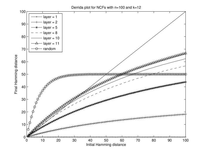
Figure 1. Derrida plots for different layer numbers. Here, $n$ is the number of nodes and $k$ is the connectivity. For each layer number, a Derrida plot was generated from 4096 random networks. The $x$-axis represents Hamming distance of pairs of states, and the $y$-axis represents Hamming distance of their images.

7. Conclusion

Nested canalizing Boolean functions were inspired by structural and dynamic features of biological networks. In this study we took a careful look at the computational properties of Boolean functions and of Boolean networks constructed from them. The main tool for our analysis is a particular polynomial normal form of the Boolean functions in question. In particular, we introduced a new invariant for nested canalizing functions, their layer number. Using it, we obtain an explicit formula of the number of nested canalizing functions, which improves on the known recursive formula. Based on the polynomial form, we also obtain a formula for the Hamming weight of a nested canalizing function. The activity number of each variable of a nested canalizing function is also provided with an explicit formula. An important result we obtain is that the average sensitivity of any nested canalizing function is less than $2$, which provides a theoretical argument why nested canalizing functions exhibit robust dynamic properties. This leads us to conjecture that the tight upper bound for the average sensitivity of any nested canalizing function is $\frac{4}{3}$.

It should be noted that all the variables in the first layer of an nested canalizing function are canalizing variables (the most dominant), all the variables in the second layer are the second most dominant, etc. The fact that networks with low layer number are more stable than those with high layer number could be a consequence of this observation, since lower layer number means more dominant variables. The most extreme examples are: when the layer number is equal to $1$, we have proved that such a function has minimal average sensitivity, therefore we also conjecture that the function with layer number number equal to $n-1$ (the maximal layer number) has maximal average sensitivity. Hence, it should be reasonable that the corresponding networks show similar behavior.

References

• [1] Kazuyuki Amano, “Tight bounds on the average sensitivity of k-CNF, ”Theory of Computing, Vol 7 (2011), pp. 45-48.
• [2] E. Balleza, E. R. Alvarez-Buylla, A. Chaos, S. Kauffman, I. Shmulevich,and M. Aldana, “Critical dynamics in genetic regulatory networks: Examples from four kingdoms, ”PLoS ONE, 3 (2008), p. e2456
• [3] C. Barrett, C. Herring, J. Reed, and B. Palsson, “The global transcriptional regulatory network for metabolism in Escherichia coli exhibits few dominant functional states, ”Proc Natl Acad Sci USA, 102 (2005), pp. 19103 19108.
• [4] E. A. Bender, J. T. Butler, “Asymptotic approximations for the number of fanout-tree functions, ”IEEE Trans. Comput. 27 (12) (1978) 1180-1183.
• [5] A. Bernasconi, “Mathematical techniques for the analysis of Boolean functions, ”Ph.D. thesis, Dipartmento di Informatica, Universita di Pisa (March, 1998).
• [6] A. Bernasconi, “Sensitivity vs. block sensitivity (an average-case study) ”Information processing letters 59 (1996) 151-157.
• [7] Ravi B. Boppana, “The average sensitivity of bounded-depth circuits ”Information processing letters 63 (1997) 257-261.
• [8] J. T. Butler, T. Sasao, and M. Matsuura, “Average path length of binary decision diagrams, ”IEEE Transactions on Computers, 54 (2005), pp. 1041 1053.
• [9] David Canright, Sugata Gangopadhyay, Subhamoy Maitra, Pantelimon St$\breve{a}$nic$\breve{a}$, “Laced Boolean functions and subset sum problems in finite fields, ”Discrete applied mathematics, 159 (2011), pp. 1059-1069.
• [10] Shijian Chen and Yiguang Hong, “Control of random Boolean networks via average sensitivity of Boolean functions, ”Chin. Phys. B Vol. 20, No 3 (2011) 036401.
• [11] Demetres Christofides, “Influences of Monotone Boolean Functions, ”Preprint 2009.
• [12] S. A. Cook, C. Dwork, R. Reischuk, “Upper and lower time bounds for parallel random access machines without simultaneous writes, ”SIAM J. Comput, 15 (1986), pp. 87-89.
• [13] B. Derrida and Y. Pomeau, “Random networks of automata: a simple annealed approximation”, Europhys, Lett., 1:45-49, 1986.
• [14] S. E. Harris, B. K. Sawhill, A. Wuensche, and S. Kauffman, “A model of transcriptional regulatory networks based on biases in the observed regulation rules, ”Complex, 7 (2002), pp. 23 40.
• [15] M. Herrgard, B. Lee, V. Portnoy, and B. Palsson, “Integrated analysis of regulatory and metabolic networks reveals novel regulatory mechanisms in saccharomyces cerevisiae, ”Genome Res, 16 (2006), pp. 627 635.
• [16] A. Jarrah, R. Laubenbacher, and A. Veliz-Cuba, “A polynomial framework for modeling and anaylzing logical models. ”In Preparation, 2008.
• [17] A. Jarrah, B. Ropasa and R. Laubenbacher, “Nested canalyzing, Unate Cascade, and Polynomial Functions”, Physica D 233 (2007), pp. 167-174.
• [18] Winfried Just, “The steady state system problem is NP-hard even for monotone quadratic Boolean dynamical systems ”Preprint,2006
• [19] Winfried Just, Ilya Shmulevich, John Konvalina, “The number and probability of canalyzing functions”, Physica D 197 (2004), pp. 211-221.
• [20] S. A. Kauffman, “The Origins of Order: Self-Organization and Selection in Evolution”, Oxford University Press, New York, Oxford (1993).
• [21] S. A. Kauffman, C. Peterson, B. samuelesson, C. Troein, “Random Boolean Network Models and the Yeast Transcription Network”, Proc. Natl. Acad. Sci 100 (25) (2003), pp. 14796-14799.
• [22] S. A. Kauffman, C. Peterson, B. Samuelsson, and C. Troein, “Genetic networks with canalyzing Boolean rules are always stable, ”, PNAS, 101 (2004), pp. 17102 17107.
• [23] S. A. Kauffman, “The large-scale structure and dynamics of gene control circuits: an ensemble approach, ”, J. Theor. Biol. 44 (1974) 167.
• [24] N.Keller and H. Pilpel, “Linear transformations on monotone functions on the discrete cube, ”Discrete Math. 309 (2009), 4210-4214.
• [25] R. Laubenbacher and B. Pareigis, “Equivenlence relations on finite dynamical systems, ”, Advances in applied mathematics 26 (2001), pp. 237-251.
• [26] W. Liu, H. L$\ddot{a}$hdedm$\ddot{a}$ki, Edward R. Dougherty and I. Shmulevich, “Inference of Boolean Networks Using Sensitivity Regularization, ”, EURASIP Journal of Bioinformatics and System Biology Volume 2008, Article ID 780541, 12 pages.
• [27] Layne, L., Dimitrova, E.S., Macauley, M. (2012). Biologically relevant properties of nested canalyzing functions. Bulletin of Mathematical Biology, 74(2), pp. 422-433.
• [28] Jiyou Li, “On the average sensitivity of the weighted sum function, ”arXiv:1108.3198v2 [cs.IT] 18 Aug 2011.
• [29] Yuan Li, “Results on Rotation Symmetric Polynomials Over $GF(p)$”, Information Sciences 178 (2008), pp. 280-286.
• [30] Yuan Li, David Murrugarra, John O Adeyeye and Reinhard Laubenbacher “Multi-State Canalyzing Functions over Finite Fields ”, http://arxiv.org/pdf/1110.6481v1.pdf
• [31] R. Lidl and H. Niederreiter, “Finite Fields”, Cambridge University Press, New York (1977).
• [32] A. A. Moreira and L. A. Amaral, “Canalyzing Kauffman networks: Nonergodicity and its effect on their critical behavior, ”, Phys. Rev. lett. 94 (21) (2005), 218702.
• [33] David Murrugarra and Reinhard Laubenbacher, “Regulatory patterns in molecular interaction networks, ”(2011), Journal of Theoretical Biology, 288, 66-72.
• [34] David Murrugarra and Reinhard Laubenbacher, “The number of multistate nested canalyzing functions, ”(2012), Physica D: Nonlinear Phenomena, 241, 921-938.
• [35] S. Nikolajewaa, M. Friedela, and T. Wilhelm, “Boolean networks with biologically relevant rules show ordered behaviorstar, open, ”Biosystems, 90 (2007), pp. 40 47.
• [36] N. Nisan, “CREW PRAMs and decision tree, ”SIAM J. Comput, 20 (6) (1991), PP. 999-1070.
• [37] Xiaoning Qian and Edward R. Dougherty, “A comparative study on sensitivitys of Boolean networks, ”978-1-61284-792-4/10 2011 IEEE.
• [38] T. Sasao, K. Kinoshita, “On the number of fanout-tree functions and unate cascade functions, ”IEEE Trans. Comput. 28 (1) (1979) 66-72.
• [39] Ilya Shmulevich, “Average sensitivity of typical monotone Boolean functions, ”arXiv:math/0507030v1 [math. Co] 1 July 2005.
• [40] Ilya Shmulevich and Stuart A. Kauffman, “Activities and sensitivities in Boolean network models, ”Physical Review Letters, Vol 93, Number 4 (2004), 048701.
• [41] Igor. E. Shparlinski, “Bounds on the Fourier coefficients of the weighted sum function, ”Information Processing Letters. 103 (2007), 83-87.
• [42] Steffen Schober and Martin Bossert, “Analysis of random Boolean networks using the average sensitivity, ”arXiv: 0704.0197v1 [nlin.CG] 2 Apr 2007.
• [43] C. H. Waddington, “Canalisation of development and the inheritance of acquired characters, ”Nature, 150 (1942), pp. 563 564.
• [44] Madars Virza, “Sensitivity versus block sensitivity of Boolean functions, ”arXiv:1008.0521v2 [cs.CC]8 Dec 2010.
• [45] Shengyu Zhang, “Note on the average sensitivity of monotone Boolean functions, ”Preprint 2011.
• [46] A. Veliz-Cuba, K. Buschur, R. Hamershock, A. Kniss, E. Wolff, and R. Laubenbacher, “AND-NOT decomposition of boolean network models”, Preprint 2012.