Line Profiles from Discrete Kinematic Data

Abstract

We develop a method to extract the shape information of line profiles from discrete kinematic data. The Gauss-Hermite expansion, which is widely used to describe the line of sight velocity distributions extracted from absorption spectra of elliptical galaxies, is not readily applicable to samples of discrete stellar velocity measurements, accompanied by individual measurement errors and probabilities of membership. These include datasets on the kinematics of globular clusters and planetary nebulae in the outer parts of elliptical galaxies, as well as giant stars in the Local Group galaxies and the stellar populations of the Milky Way. We introduce two parameter families of probability distributions describing symmetric and asymmetric distortions of the line profiles from Gaussianity. These are used as the basis of a maximum likelihood estimator to quantify the shape of the line profiles. Tests show that the method outperforms a Gauss-Hermite expansion for discrete data, with a lower limit for the relative gain of $\approx 2$ for sample sizes $N\approx 800$. To ensure that our methods can give reliable descriptions of the shape, we develop an efficient test to assess the statistical quality of the obtained fit.

As an application, we turn our attention to the discrete velocity datasets of the dwarf spheroidals (dSphs) of the Milky Way. Sculptor and Fornax have datasets of $\gtrsim 1000$ line of sight velocities of probable member stars. In Sculptor, the symmetric deviations are everywhere consistent with velocity distributions more peaked than Gaussian. In Fornax, instead, there is an evolution in the symmetric deviations of the line profile from a peakier to more flat-topped distribution on moving outwards. Although the datasets for Carina and Sextans are smaller, they still comprise several hundreds of stars. Our methods are sensitive enough to detect evidence for velocity distributions more peaked than Gaussian. These results suggest a radially biased orbital structure for the outer parts of Sculptor, Carina and Sextans. On the other hand, tangential anisotropy is favoured in Fornax. This is all consistent with a picture in which Fornax may have had a different evolutionary history to Sculptor, Carina and Sextans.

1 Introduction

Our ability to uncover the elusive properties of dark matter in galaxies is based on the analysis of velocities of stars. For the case of pressure-supported systems like elliptical galaxies, a great advantage is obtained by considering the properties of the entire line profile – that is, the shape of the line of sight velocity distributions $\mathscr{L}(v)$ – rather than just the first two velocity moments. This helps break the pernicious mass-anisotropy degeneracy, which otherwise enables dark matter mass to be traded against velocity anisotropy at both small and large radii, and hence hidden away.

For elliptical galaxies, higher order velocity information can be extracted from absorption line spectra. The shape of the velocity distributions is usually quantified within the framework of a Gauss-Hermite series, introduced in Gerhard (1993) and van der Marel & Franx (1993). Given the velocity distribution $\mathscr{L}(v)$, the associated Gauss-Hermite series is defined by the relation

$$\mathscr{L}(v)={\gamma\over{\sqrt{2\pi\sigma^{2}}}}{\exp\left[-{1\over 2}\left({{v\!-\!\mu}\over\sigma}\right)^{2}\right]}\left\{1\!+\!\sum_{i=3}^{n}h_{i}H_{i}\left({{v\!-\!\mu}\over\sigma}\right)\right\}$$ (1)

in which the parameters $\gamma$, $\mu$ and $\sigma$ identify respectively the normalization, mean and standard deviation of the best fitting Gaussian, while the coefficients $h_{i}$ specify the shape information. The advantage of this formalism is that Hermite polynomials $H_{i}$ are orthonormal with respect to a Gaussian weight function. The (lowest order) Gauss-Hermite moments measure structure in the central parts of the velocity distribution and have a limited dependence on the poorly-determined tails.

However, a disadvantage of the Gauss-Hermite formalism is that it cannot be easily applied to the large class of problems in which the kinematic observations come in the form of discrete velocity measurements, rather than as line of sight velocity distributions extracted from absorption spectra. This includes the modelling of the dynamics of galaxies at large radii, where integrated-light spectroscopy is not possible because of low surface brightness. Here, tracers such as globular clusters and planetary nebulae are used to probe the realm of dark matter (e.g., Romanowsky et al., 2003; Coccato et al., 2009; Napolitano et al., 2011; Deason et al., 2012). In the Local Group, ground-based observations of nearby dwarf spheroidal galaxies and globular clusters have enabled impressive datasets of up to thousands of individual line of sight velocities to be gathered (e.g., Kleyna et al., 2002, 2004; Wilkinson et al., 2004; Battaglia et al., 2006; Reijns et al., 2006; Battaglia et al., 2008; Walker et al., 2009, 2010). Clusters of galaxies provide another example in which the kinematic information is available as discrete velocities (e.g., Łokas & Mamon, 2003; Wojtak & Łokas, 2010).

For such datasets, the Gauss-Hermite formalism has shortcomings that limit both accuracy and precision. Difficulties are mainly connected with the heterogeneous observational uncertainties and the probabilities of membership. Additionally, a straightforward implementation of the methods of Gerhard (1993) and van der Marel & Franx (1993) is only possible for continuous data, thus introducing the potentially important loss of information due to data binning. In general, a dataset of discrete velocities $\vec{V}=\{v_{1},\cdots,v_{N}\}$ comes together with a set of observational uncertainties $\vec{\Delta}=\{\delta_{1},\cdots,\delta_{N}\}$, the values of which are usually inhomogeneous. Also, the different kinematic tracers may have different probabilities of membership, $\vec{P}=\{p_{1},\cdots,p_{N}\}$, which should also be included. It is difficult to account properly for this information within the framework of a Gauss-Hermite series, as the binning procedure erases virtually everything except $\vec{V}$. For this reason, the accuracy of the results obtained can be seriously diminished if the observational uncertainties are large (in terms of the intrinsic dispersion $\sigma_{\rm int}$), and/or if either the observational uncertainties themselves or the membership probabilities are highly inhomogeneous.

Furthermore, whatever the sample size $N$, the shape measured within the Gauss-Hermite framework is not the shape of the intrinsic velocity distribution $\mathscr{L}$ itself, but rather the shape of its convolution with the uncertainties’ kernel, often taken to be Gaussian. This causes an attenuation of the signal due to the intrinsic deviations from Gaussianity in $\mathscr{L}$. The magnitude of this attenuation needs to be separately quantified and then simulated on models before direct comparison with the observables, which is a lengthy procedure.

Given these difficulties, it is clear that a feasible solution might be to use Bayesian methods, which naturally allow us to include all available information, such as uncertainties of any origin, as well as probabilities of membership. Unfortunately, the Gauss-Hermite series is not always positive definite and so does not itself define proper probability distributions. In order to implement a maximum-likelihood method, we will have to introduce a new suitable parametrization. At first glance, this may be viewed as a limitation of a Bayesian framework, since any parametric family of velocity distributions may not be flexible enough to describe the dataset. However, we put in place an analytic device that allows us to test directly whether the description of the observational sample that is recovered within a parametric family is a good statistical description or not. Hence, it is always possible to identify whether the adopted parametrization is suitable.

As an application for our new methods, we turn our attention to the highly dark matter dominated dwarf spheroidal galaxies (dSphs) of the Milky Way. Here, the goal is to map out the density distribution of the dark matter and compare it to the theoretical predictions of hierarchical cosmologies. Sometimes, as in the nearby Sculptor dSph, the properties of the dark halo profile have been strongly constrained by exploiting the fortunate coexistence of multiple stellar populations, having different metallicities and kinematics (Battaglia et al., 2008; Walker & Peñarrubia, 2011; Amorisco & Evans, 2012), whilst de Boer et al. (2012) have mapped out the detailed star formation history. Jardel & Gebhardt (2012) have recently shown for the Fornax dSph, that even with just one (perhaps composite) stellar population, the detailed modelling of the velocity distributions may be able to constrain tightly the mass profile. A key ingredient here is the use of the shape information of the line profiles in addition to the second moments familiar from straightforward Jeans equation modelling (e.g. Gilmore et al., 2007; Walker et al., 2010). By themselves, the Jeans equations do not provide enough information to permit the dark matter distribution to be mapped out unambiguously (Evans et al., 2009).

We use our new methods to analyze the discrete velocity datasets of four dSphs – Sculptor, Carina, Sextans and Fornax – and obtain for the first time detailed measurements of the higher velocity moments. This information provides powerful observables for future dynamical analyses of the dSphs, and will help constrain the mass profiles in these systems. Also, since the the formation history of dSphs is mirrored in their current orbital structure, detailed information on the line profiles will identify and constrain feasible formation mechanisms.

The plan of the paper is as follows. In Section 2, we investigate the magnitude of different effects that influence any velocity distribution measurement, such as limited sampling, observational uncertainties and – for line of sight distributions – apparent rotation due to systematic proper motion. In Section 3, we construct suitable two-parameter families of distributions to use in a Bayesian likelihood. We describe the method through which we control the statistical meaningfulness of the maximum likelihood fit. Section 4 deals with the application of the maximum likelihood measurements of the higher velocity moments to the dSphs.

2 Achievable Accuracy

Reconstructing the intrinsic velocity distribution $\mathscr{L}(v)$ of a stellar system is a complex task, since several different effects can modify the signal that we actually observe. The purpose of this Section is to quantify these contributions.

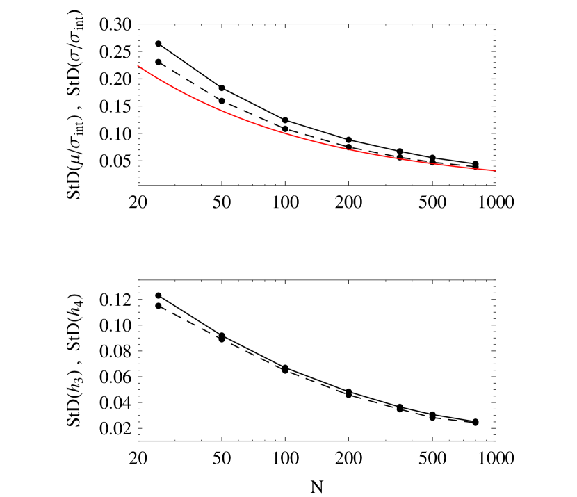
Figure 1: Accuracy limits from limited sampling. Upper panel: the evolution of the standard deviation of the estimated (normalized) mean $\mu$ (full line) and dispersion $\sigma$ (dashed line) with the sample size $N$. In red, the representative behaviour of $1/\sqrt{N}$ is shown. Lower panel: the evolution of the standard deviation of the Gauss-Hermite moments $h_{3}$ (full line) and $h_{4}$ (dashed line) with the sample size N.

2.1 Intrinsic noise from limited sampling

The most obvious difficulty in measuring the shape of the velocity distribution in astrophysical systems is limited sampling. Finite samples of velocities naturally introduce some noise, which may be able to alter completely the intrinsic shape.

In general, the magnitude of the noise has its strongest dependence on the sample size $N$. Hence, the number of available kinematic tracers poses a limit to the level of achievable accuracy. Some, smaller dependence can also be ascribed to the method we use to measure such a shape. In this Section, we use the Gauss-Hermite expansion introduced in Gerhard (1993) and van der Marel & Franx (1993). Later, we will compare these results to our maximum likelihood method.

As a representative case, we assume that the intrinsic velocity distribution $\mathscr{L}$ is a perfect Gaussian, $\mathscr{G}(\mu_{\rm int},\sigma_{\rm int})$, where $\mu_{\rm int}$ and $\sigma_{\rm int}$ are its intrinsic mean and dispersion. We generate synthetic samples of size $N$, namely $\vec{V}=\{v_{1},\cdots,v_{N}\}$, which share the distribution $\mathscr{L}(v)=\mathscr{G}(\mu_{\rm int},\sigma_{\rm int})$. For each of them, we measure the standard set of properties: $(\mu,\sigma,h_{3},h_{4})$, namely the estimated mean, dispersion, and the first non-zero Gauss-Hermite moments, $h_{3}$ and $h_{4}$.

For the sake of clarity, the pair $(\mu,\sigma)$ identifies the best Gaussian fit $\mathscr{G}(\mu,\sigma)$ to the binned dataset $\vec{V}$ (we do not report results related to the much less interesting normalization of the Gaussian fit). The Gauss-Hermite moments are computed as in van der Marel & Franx (1993), hence $h_{1}$ and $h_{2}$ are identically zero. We adapt the size of the bin $s_{\rm bin}$ to the size of the sample $N$ with the standard prescription $s_{\rm bin}\propto N^{-1/3}$. The bins are centered on the sample mean, and, as a reference, for our smallest sample size $N=25$ we use $\approx 4$ bins within the interval $(-\sigma,\sigma)$.

For any sample size, we quantify the noise due to limited sampling by repeating this measurement procedure on a large number of synthetic samples. Fig. 1 shows as a function of sample size $N$, the variation in the standard deviation (StD) of the estimated (normalized) mean $\mu/\sigma_{\rm int}$, (normalized) dispersion $\sigma/\sigma_{\rm int}$, and Gauss-Hermite moments $h_{3}$ and $h_{4}$. As expected, StD$(\mu/\sigma_{\rm int})$ and StD$(\sigma/\sigma_{\rm int})$ follow approximately the reference prescription StD$\sim 1/\sqrt{N}$. Note though, that while StD$(\sigma/\sigma_{\rm int})<$ StD$(\mu/\sigma_{\rm int})$, it does not achieve the statistical prescription StD$(\sigma)\sim 1/\sqrt{2N}$. More significant, however, is the result for the Gauss-Hermite moments. We find that, up to a sample size of $N=200$, the magnitude of the noise (${\rm StD}(h_{3})\approx{\rm StD}(h_{4})\approx 0.05$) is higher than the amount of intrinsic signal that one, in general, can typically expect to find in galactic astronomy. This result is approximately independent of the intrinsic shape of the velocity distribution: we find that the accuracy limits quantified here remain substantially unchanged for synthetic datasets extracted from non-Gaussian distributions. As a consequence, for sample sizes less than 200, the accuracy of any measurement is potentially very low, which casts doubts on the reliability of results obtained using just a few tens of tracers.

In fact, the situation is even worse, as the intrinsic signal in $\mathscr{L}$ is also attenuated by the observational uncertainties on the discrete kinematic measurements. Thus, it is highly likely that any deviation from Gaussianity detected in small samples is an artefact of under-sampling and/or binning, rather than being real. We conclude that it is extremely difficult to measure reliably the shape of any velocity distribution $\mathscr{L}$ with a sample size that is significantly smaller than $N=200$. In the following, we will only consider samples with $N\geq 200$.

2.2 Signal attenuation by observational uncertainties

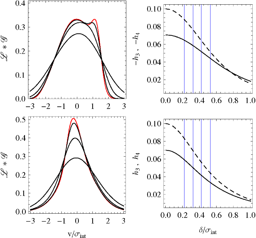
Figure 2: The effect of observational uncertainties. Left panels: the black full curves show the evolution of $\mathscr{L}\ast\mathscr{G}$ for increasing levels of observational uncertainty. $\mathscr{L}$ is the intrinsic velocity distribution displayed in red. The adopted values of $\delta/\sigma_{\rm int}$ are $\{0.2,0.5,1\}$. Right panels: the corresponding evolution of the Gauss-Hermite moments $h_{3}$ (full line) and $h_{4}$ (dashed line). Blue vertical lines illustrate the level of observational uncertainty, from left to right, of the Fornax, Sculptor, Sextans and Carina datasets from Walker et al. (2009).

Inevitably, any real dataset $\vec{V}$ has its own set of observational uncertainties $\vec{\Delta}=\{\delta_{1},\cdots,\delta_{N}\}$. Their effect is to alter the observed velocity distribution, so that the $i$-th star is in fact associated with the velocity distribution $\mathscr{L}\ast\mathscr{G}(0,\delta_{i})$, rather than with the intrinsic $\mathscr{L}$ itself. By $\mathscr{L}\ast\mathscr{G}$, we indicate the convolution of the velocity distribution $\mathscr{L}$ with the Gaussian kernel $\mathscr{G}$:

$$\left[\mathscr{L}\ast\mathscr{G}\right](v)=\int_{-\infty}^{\infty}dx\ \mathscr{L}(x)\ {{\exp{\left[-{1\over 2}\left({{v-x}\over\delta_{i}}\right)^{2}\right]}}\over{\sqrt{2\pi\delta_{i}^{2}}}}$$ (2)

Unsurprisingly, the effect of this convolution is to attenuate the features of $\mathscr{L}$.

For a given velocity distribution $\mathscr{L}(v)$, the magnitude of this attenuation is a function of the dimensionless ratio observational uncertainty to the intrinsic dispersion $\delta/\sigma_{\rm int}$ only. For any sample size $N$, it is impossible to resolve the intrinsic velocity distribution $\mathscr{L}$ with the Gauss-Hermite method used in previous Section 2.1. Rather, the measured signal is the one corresponding to $\mathscr{L}\ast\mathscr{G}(0,\delta_{m})$, where $\delta_{m}$ is, approximately, the mean of the sample of uncertainties $\vec{\Delta}$.

As an example, let us consider two arbitrary velocity distributions $\mathscr{L}(v)$ both sharing the same amount of non-Gaussianity as characterized by their Gauss-Hermite expansion: the first has $(h_{3},h_{4})=(-0.07,-0.1)$, and the second has $(h_{3},h_{4})=(0.07,0.1)$. They are displayed as red full curves in the upper and lower left panels of Fig. 2. The right panels show the evolution of the Gauss-Hermite moments $h_{3}$ (full line) and $h_{4}$ (dashed line) as functions of observational uncertainty on the kinematic measurements $\delta/\sigma_{\rm int}$. Clearly, these are monotonic functions that tend to zero for both Gauss-Hermite moments – that is to a perfect Gaussianity – when $\delta/\sigma_{\rm int}\gtrsim 1$ or when the uncertainty is high enough to overwhelm any signal in $\mathscr{L}$. The black curves in the left panels illustrate this process by showing $\mathscr{L}\ast\mathscr{G}$ when $\delta/\sigma_{\rm int}\in\{0.2,0.5,1\}$.

From Fig. 2, it is clear that the effect of attenuation is significant. The vertical lines in the right panels show the levels of average observational uncertainty $\delta_{m}/\sigma_{\rm int}$ for the datasets on the Galactic dwarf spheroidals presented by Walker et al. (2009). Specifically, from the lowest to highest levels of uncertainty, we find

$${\rm Fornax:} \delta_{m}/\sigma_{\rm int}\approx 0.22$$

$${\rm Sculptor:} \delta_{m}/\sigma_{\rm int}\approx 0.33$$

$${\rm Sextans:} \delta_{m}/\sigma_{\rm int}\approx 0.42$$

$${\rm Carina:} \delta_{m}/\sigma_{\rm int}\approx 0.53$$

Taking the case of Sculptor as an example and consulting Fig. 1, it is clear that even the strong signal adopted here ($|h_{4}|=0.1$) would remain smaller than (or comparable with) the noise from limited sampling up to $N\approx 100$. On the other hand, by reversing the argument, if the typical ultrafaint has a kinematic sample of $N\lessapprox 100$, any signal would be overwhlemed by the shot noise unless $\delta_{m}/\sigma_{\rm int}\lessapprox 0.25$. Although important improvement has been achieved (see for example Koposov et al., 2011), significantly larger datasets would be necessary to resolve the line profile information in such systems. Finally, let us note that if we compare the observed shape of $\mathscr{L}\ast\mathscr{G}$ with that of theoretical dynamical models, we must account for this inevitable attenuation effect. Whether using a Gauss-Hermite expansion or a non-parametric reconstruction of the velocity distribution $\mathscr{L}(v)$ – as in Jardel & Gebhardt (2012) – this attenuation must be applied to the dynamical models themselves before comparison with the observables. On the other hand, a maximum likelihood approach allows us to take into account the observational uncertainties while deriving our observables, and thus we are able to reconstruct the properties of $\mathscr{L}$ itself, rather than those of $\mathscr{L}\ast\mathscr{G}$.

2.3 Apparent rotation from global proper motion

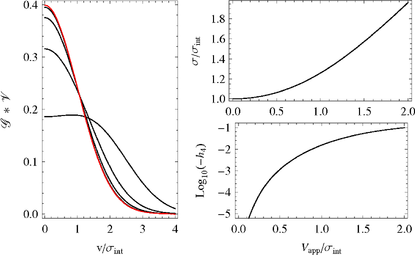
Figure 3: The effect of apparent rotation. Left panel: an intrinsic Gaussian velocity distribution $\mathscr{L}=\mathscr{G}(0,\sigma_{\rm int})$ (red curve) disturbed by apparent rotation of growing amplitude $V_{\rm app}/\sigma_{\rm int}\in\{0.2,0.5,1,2\}$ (black curves). Right panels: the evolution of the dispersion $\sigma$ of the best-fitting Gaussian and of the first nonzero Gauss-Hermite moment $h_{4}$ for different $V_{\rm app}/\sigma_{\rm int}$.

The exploitation of the projection effect that causes an extended object in the sky to have an apparent line-of-sight solid-body rotation as a consequence of its global proper motion has a long history (e.g., Feast et al., 1961). Very recently, the effect has been exploited by Walker et al. (2008) to derive the systemic proper motion of the Fornax, Sculptor Carina and Sextans dSphs.

For our purposes, apparent rotation is a potentially dangerous effect because it alters the shape of the observed velocity distribution. In particular, for the line of sight velocity distribution $\mathscr{L}$, the contribution of apparent rotation is degenerate with the signal produced by tangential anisotropy. For this reason, whenever possible, apparent rotation is usually subtracted from the dataset before estimating the shape of $\mathscr{L}$. Nonetheless, it is useful to have an understanding of this spurious effect, since the subtraction of the apparent velocity field from the dataset does come at a price. It may, in fact, not be worthwhile degrading each discrete velocity measurement with the uncertainty of the apparent velocity field if the effect on $\mathscr{L}$ is expected to be exceedingly small.

For simplicity, we consider the case in which the sample of kinematic tracers is uniformly distributed on a circle. This assumption mimics the more realistic case of a thin circular annulus. Let us use the notation

$$v_{\rm app}(R,\theta)=c\ D\ \vec{\mu}\cdot\vec{R}=V_{\rm app}\ \sin(\theta-\theta_{\rm app})$$ (3)

where $\vec{\mu}$ is the proper motion, $D$ is the distance, $\vec{R}$ is the projected distance on the sky (measured in arcmin), $\theta_{\rm app}$ identifies the apparent rotation axis, and $c$ is a constant ($c=1.379\cdot 10^{-5}$ (km century)/(s kpc arcmin mas)). Hence, $V_{\rm app}$ represents the maximum apparent rotation velocity attainable at the projected radius $R$. If $\mathscr{L}$ is the intrinsic velocity distribution of the tracers on the circle with radius $R$, then the effective velocity distribution we observe is $\mathscr{L}\ast\mathscr{V}(V_{\rm app})$, where

$$\mathscr{V}(V_{\rm app})=\begin{cases}{\left(\pi V_{\rm app}\sqrt{1-v^{2}/V^{2}_{\rm app}}\right)^{-1}}&{\rm if}\ |{v/V_{\rm app}}|\leq 1\\ 0&{\rm if}\ |{v/V_{\rm app}}|>1\end{cases}$$ (4)

is the velocity distribution associated with the apparent rotation.

The magnitude of the deviations from $\mathscr{L}$ introduced by the convolution is a function of the ratio $V_{\rm app}/\sigma_{\rm int}$ only. Fig. 3 illustrates the representative case in which $\mathscr{L}=\mathscr{G}(0,\sigma_{\rm int})$. The left panel illustrates four different velocity distributions $\mathscr{G}\ast\mathscr{V}(V_{\rm app})$, obtained for $\mathscr{V}_{\rm app}/\sigma_{\rm int}\in\{0.2,0.5,1,2\}$. As anticipated, deviations from the pure Gaussian case (in red) are towards a flat topped velocity distribution and even a double peaked structure appears at higher levels of apparent rotation. Both these features are usually considered indicative of tangential velocity anisotropy, though clearly this is not the case here. The panels on the right quantify the effect of apparent rotation on the dispersion of the best fitting Gaussian $\sigma$ and on the Gauss-Hermite moment $h_{4}$. Since both $\mathscr{G}$ and $\mathscr{V}$ are even functions, $h_{3}$ is identically zero. Both $\sigma$ and $h_{4}$ are more strongly modified as the magnitude of the apparent rotation increases.

For the dSphs considered later in this paper, the effect is actually very small. Sculptor and Fornax are the only dSphs where a reliable non-zero estimate of the rotation signal can presently be obtained. Even at large distances $R$, the amount of apparent rotation $V_{\rm app}$ (less than a few kms^-1) still remains just a fraction of the intrinsic dispersion $\sigma_{\rm int}$ (typically $\sim 10$ kms^-1). Unless we have a very large sample size, the modifications introduced by apparent rotation are smaller than the achievable accuracy. As Fig. 3 shows, this is particularly true for the Gauss-Hermite moment $h_{4}$, which remains virtually unaffected up to $V_{\rm app}/\sigma_{\rm int}\approx 0.7$, even with sample sizes as large as $N=800$.

This is clearly not a general rule, and Fig. 3 can be used to assess other cases, such as nearby globular clusters. Also, there may be reasons that justify the subtraction of the apparent rotation from the kinematic dataset, as for example if the considered annuli are highly non-uniformly populated, or if other spatial regions are considered in the place of annuli, or if the estimate of the apparent velocity field is precise enough.

3 Maximum likelihood method

3.1 Introduction

Suppose we have a set of $N$ kinematic tracers with velocities $\vec{V}=\{v_{1},\cdots,v_{N}\}$, which are aligned along the same axis, for example, the line of sight direction. We assume that they sample a specified spatial region, the velocity distribution of which we want to determine. The set $\vec{V}$ is accompanied by the set of velocity uncertainties $\vec{\Delta}=\{\delta_{1},\cdots,\delta_{N}\}$, and membership probabilities $\vec{P}=\{p_{1},\cdots,p_{N}\}$. We take these probabilities as assigned constants, although in some cases the probability $p_{i}$ may be modelled as a function of the velocity $v_{i}$ as well as of other observable quantities in order to identify foreground objects, separate stellar populations and so on.

Now suppose we have at our disposal a family of velocity distributions $\mathscr{L}(v)$. This is associated with a set of parameters $\vec{\Theta}=\{\theta_{1},\cdots,\theta_{j}\}$. Within this family, we can recover the best statistical description of the sample $\vec{V}$ by maximizing the likelihood:

$$L(\vec{\Theta})=\prod_{i=1}^{N}\ p_{i}\ \left[\mathscr{L}(\vec{\Theta})\ast\mathscr{G}(0,\delta_{i})\right](v_{i})\ ,$$ (5)

in which we have implicitly assumed that the distributions $\mathscr{L}$ have unit integral.

In the case of a Gauss-Hermite expansion, the set $\vec{\Theta}$ comprises the dimensional pair $(\mu,\sigma)$ of the best Gaussian fit, together with the series of dimensionless moments $h_{j}$, truncated according to the size of the dataset as well as to the uncertainties of the kinematic measurements. Note that in the terminology of van der Marel & Franx (1993), $\mu$ and $\sigma$ represents the mean and dispersion of the best-fitting Gaussian.

In this paper, however, we prefer to use $\mu$ and $\sigma$ to denote the first and second moment of the distribution $\mathscr{L}$:

$$\mu = \int_{-\infty}^{\infty}\ \mathscr{L}(\vec{\Theta};v)\ v\ dv\ ;$$ (6)

$$\sigma^{2} = \int_{-\infty}^{\infty}\ \mathscr{L}(\vec{\Theta};v)\ v^{2}\ dv\ .$$ (7)

We can highlight the role of these two dimensional quantities in the likelihood (5) by separating them from the remaining shape parameters in $\vec{\Theta}$, which we group in the subset $\vec{\Theta}_{\rm sh}$, to yield

$$L(\vec{\Theta})=\prod_{i=1}^{N}\ {p_{i}\over\sigma}\ \left[\mathscr{L}(\vec{\Theta}_{\rm sh})\ast\mathscr{G}(0,\delta_{i})\right]\left({{v_{i}-\mu}\over\sigma}\right)\ .$$ (8)

We have made explicit use of the fact that the distributions $\mathscr{L}(\vec{\Theta}_{\rm sh};v)$ have zero mean, unit integral and unit dispersion. Finally, we will use the notation $e_{\theta}$ for the uncertainty of the parameter $\theta\in\vec{\Theta}$. This uncertainty is defined by the 68% confidence region associated with the marginalized likelihood.

The implementation of a maximum likelihood method for measuring the shape of velocity distributions $\mathscr{L}$ brings about a number of advantages. The most evident one is the elimination of any arbitrary aspect introduced by binning in velocity space. Of equal importance is the problem of observational uncertainties. These are not easily – nor usually – taken into account by the binning procedure, hence making any measurement questionable. The method of maximum likelihood instead furnishes a natural way to incorporate any uncertainty into the measurement procedure. Also, we can reconstruct directly the intrinsic velocity distribution $\mathscr{L}$, rather than the attenuated one $\mathscr{L}\ast\mathscr{G}(0,\delta_{m})$. This has two consequences. First, the limit in accuracy due to sampling (see Sect. 2.1) is less important, since intrinsic signals are stronger. Second, observables obtained in this way can be directly compared with dynamical models. This is not possible in general, since if $\mathscr{L}\ast\mathscr{G}(0,\delta_{m})$ is reconstructed, this should be compared with an analogous quantity which is only indirectly provided by the models.

Given these advantages, it is natural to look for an implementation of the maximum likelihood approach using the standard Gauss-Hermite expansion. Such an approach has been proposed in van de Ven et al. (2006) and used in Rangwala et al. (2009) to characterize the kinematics of the Galactic bar. Particular attention must be devoted to the tails of the velocity distributions, as a truncated Gauss-Hermite series is not always positive definite and so cannot be used as a probability distribution. In order to circumvent these difficulties, we construct alternative families of probability distributions $\mathscr{L}(\vec{\Theta}_{\rm sh};v)$, and it is to this problem we now turn.

3.2 A Two-Parameter Family of Velocity Distributions

For velocity distributions $\mathscr{L}$, it is useful to start with a Gaussian profile $\mathscr{G}$, since it represents a good approximation for most realistic cases. We maintain this perspective, but adopt two additional parameters to measure the deviations from a pure Gaussian profile. The parameter $s$ quantifies the magnitude of the symmetric deviations, the parameter $a$ the magnitude of asymmetric deviations. This is in addition to the parameters $\mu$ and $\sigma$, which are the mean and the dispersion of any distribution $\mathscr{L}$. For the sake of clarity:

$$\vec{\Theta}=\{\mu,\sigma\}\cup\vec{\Theta}_{\rm sh}=\{\mu,\sigma,{s},{a}\}\ .$$ (9)

As in any parametric approach, the choice of the adopted model is a crucial step. In the next subsections, we propose families of velocity distributions encompassing a wide range of deviations from the Gaussian profile seen in typical stellar dynamical systems.

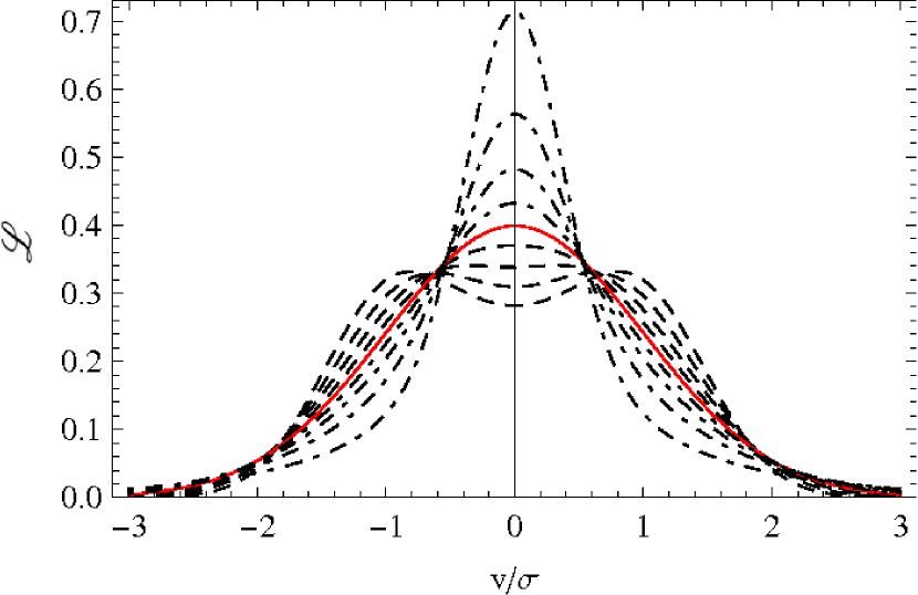
Figure 4: Our one-parameter family of symmetric velocity distributions. The red profile illustrates a perfect Gaussian; dashed profiles display negative values of $s$, ranging in the interval $[-4,0)$; dotdashed profiles display positive values of $s$ ranging in the interval $(0,0.8]$.

Figure 5: An illustration of our final parametrization of asymmetric deviations. In each of the three panels, which display the cases $s\in\{0.5,0,-0.5\}$, the red profile illustrates the symmetric distribution $\mathscr{L}(s,a=0;v)$; black profiles display the growth of asymmetries as measured by our parameter $a$, for $a\in\{0.1,0.3,0.7\}$.

3.2.1 Symmetric deviations

In order to build a set of representative, symmetric, non-Gaussian velocity distributions, we exploit the three-dimensional distribution of velocities

$$f(v_{r},|\vec{v}_{t}|)={{|\vec{v}_{t}|^{-2{s}}}\over{\rho({s})}}\exp\left[-{{v^{2}_{r}+|\vec{v}_{t}|^{2}}\over{2\sigma^{2}_{r}}}\right]\ ,$$ (10)

in which $v_{r}$ and $\vec{v}_{t}$ are respectively the radial and tangential components of the velocity, $s$ is our free parameter for symmetric deviations (${s}=0$ identifies the Gaussian case) and $\rho({s})$ is defined so that $\int fd^{3}\vec{v}=1$:

$$\rho({s})=\sqrt{2\pi}\sigma_{r}^{3}\ (2\sigma_{r}^{2})^{-{s}}\ \Gamma(1-{s})\ .$$ (11)

The simple model of eqn (10) is familiar from constant anisotropy models $\beta={s}$, where, with the usual notation, $\beta=1-\sigma^{2}_{t}/2\sigma^{2}_{r}$. In particular, these three-dimensional or intrinsic velocity distributions are the constant anisotropy phase space distribution functions for the isothermal sphere (see e.g., Gerhard, 1991; Evans, 1994). This seems a natural starting point for galaxies with flattish velocity dispersion profiles, for which we might plausibly expect the intrinsic velocity distributions to be reasonably similar.

Our family of symmetric velocity distributions corresponds to a set of line of sight velocity distributions generated by $f$. The direction associated with the line of sight identifies the velocities $v_{\parallel}$ and $\vec{v}_{\perp}$. If $\varphi$ is the angle defined by the line of sight and its projection onto the plane of the tangential velocity $\vec{v}_{t}$, we have that

$$\left\{\begin{array}[]{lclcl}v_{r}&=&|v_{\perp}|\cos(\alpha)\cos(\varphi)&+&v_{\parallel}\sin(\varphi)\\ v_{\theta}&=&|v_{\perp}|\cos(\alpha)\sin(\varphi)&-&v_{\parallel}\cos(\varphi)\\ v_{\phi}&=&|v_{\perp}|\sin(\alpha)&&\end{array}\right.\ .$$ (12)

This set of linear transformations allows us to compute the line of sight distribution generated by $f$ for any direction $\varphi$:

$$f_{los}(v_{\parallel},\varphi) = \int d^{2}\vec{v}_{\perp}\ f\left[v_{r}(v_{\parallel},\vec{v}_{\perp}),v_{t}(v_{\parallel},\vec{v}_{\perp})\right]\ ,$$

$$= \int_{0}^{\infty}dv_{\perp}\int_{0}^{2\pi}d\alpha\ v_{\perp}f(v_{r},|v_{t}|)\ .$$

Given the properties of the pressure tensor of $f$, the line of sight distribution $f_{\rm los}$ has a dispersion

$$\sigma_{\parallel}(\varphi)=\sigma_{r}\sqrt{1-{s}\cos(\varphi)^{2}}.$$ (14)

Hence, the distributions defined by

$$\mathscr{L}({s},\varphi;v)=\sigma_{\parallel}(\varphi)\cdot f_{los}[\sigma_{\parallel}(\varphi)\cdot v]$$ (15)

have by construction zero mean, unit integral and unit dispersion, and are well-suited for our maximum likelihood method.

By reporting explicitly all functional dependences in eqn (15), we highlight the fact that the distributions $\mathscr{L}$ have two parameters, namely the shape $s$ and the angle $\varphi$. The parameter $s$ is associated with genuine deviations from the Gaussian profile, while the effect of varying $\varphi$ between 0 and $\pi/2$ at fixed $s$ is to erase these deviations ($\varphi=\pi/2$ identifies the radial direction, whose line of sight distribution is Gaussian for any $s$). For this reason, $s$ and $\varphi$ cannot be maintained as independent parameters – since they are strongly correlated – and a prescription of the form $\varphi=\varphi({s})$ is needed as a ‘closure’. Different prescriptions introduce small differences in the resulting family of distributions, but in this paper we adopt

$$\cos[\varphi({s})]\equiv 15/(16-{s})\$$ (16)

for two different reasons. First, for positive $s$, this allows us to keep non Gaussianities as strong as possible when $s$ approaches its upper limit of unity $\varphi(s=1)=0$. At the same time, we avoid setting $\varphi$ uniformly to zero, since this produces distributions with strongly pronounced peaks also for much smaller values of $s$. Second, the closure condition (16) allows us, for negative values of $s$, to provide a range of flat topped distributions before a double peaked structure appears. Flat topped distributions are almost absent if $\varphi$ is uniformly set to zero. Fig. 4 illustrates the family of symmetric distributions $\mathscr{L}$ we have defined here. Both the characteristic extremes of a spiky distribution with substantial tails and of a double peaked structure with sharp edges can be clearly identified within the displayed range $-4\leq s\leq 1$. Between such extremes, the entire range of intermediate configurations is accessible as well.

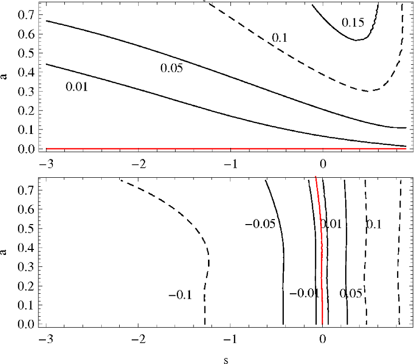
Figure 6: A comparison with Gauss-Hermite moments. The upper and lower panels show contours of the Gauss-Hermite moments $h_{3}$ and $h_{4}$ for our two parameter family of distributions. To guide the eye, the contours corresponding to $0$ and to $0.1$ are marked, respectively, in red and dashed lines.

3.2.2 Asymmetric deviations

Asymmetric distributions can be derived from our symmetric distributions $\mathscr{L}({s};v)$ by the transformation

$$\mathscr{L}^{\prime}({s},{a};v)=\mathscr{L}({s};{\rm X}({s},{a};v)).$$ (17)

The asymmetric deviations are introduced by the map $v\rightarrow{\rm X}({s},{a};v)$. The basic ingredients of the function ${\rm X}$ enabling it to deliver well behaved distributions within the entire parameter space $({s},{a})$ are described in Appendix A. Here, we only report our choice:

$${\rm X}\equiv{{a}\over{|{a}|}}\left\{v\!-\!|{a}|\ e^{\left[-\left({{v-|{a}|}\over{1/2+3|{a}|}}\right)^{4}\right]}\left({v\over{1\!+\!{s}/6\!+\!|{a}|}}\!+\!{{|{a}|}\over 2}\!-\!{3\over 2}\right)\right\}\ .$$ (18)

While introducing asymmetries, the application of the transformation (18) to the symmetric distributions $\mathscr{L}$ also alters the normalization, so that in general $\mathscr{L}^{\prime}$ is no longer a zero-mean, unit-integral and unit-dispersion distribution. However, it is straightforward to account for these matters and we define our final two-parameters family as

$$\mathscr{L}({s},{a};v)\equiv{{\sigma^{\prime}}\over{I^{\prime}}}\mathscr{L}^{\prime}({s},{a};\sigma^{\prime}\cdot v+\mu^{\prime})\ ,$$ (19)

where $\mu^{\prime}$, $\sigma^{\prime}$ and $I^{\prime}$ are respectively the mean, dispersion and integral of the distribution $\mathscr{L}^{\prime}$ in eqn (17). Fig 5 displays a few examples of asymmetric velocity distributions contained in our two-parameters family. The different panels illustrate the asymmetric deviations caused by positive values of ${a}$ for three different values of ${s}\in\{0.5,0,-1\}$.

3.2.3 The Gauss-Hermite moments

To establish a quantitative comparison with the standard Gauss-Hermite expansions, we measure the first two nonzero moments $h_{3}$ and $h_{4}$ of our family of distributions. Each of them is a function of our two parameters ${s}$ and ${a}$, namely

$$h_{3}={a}/|{a}|\ H_{3}({s},|{a}|)\ ;\qquad\qquad h_{4}=H_{4}({s},|{a}|)\ .$$ (20)

Contours of $H_{3}$ and $H_{4}$ in the $({s},{a})$ plane are displayed in the upper and lower panel of Fig 6. In both cases, the reference values of $0$ and $0.1$ are highlighted respectively by a red full line and a dashed line to guide the eye.

There are some aspects worth noting. The amount of asymmetric deviation as quantified by $h_{3}$ is a function of both ${a}$ and ${s}$. As is evident from the contours of $H_{3}$, it is not possible to define a one-to-one correspondence ${a}\leftrightarrow h_{3}$. However, at least in the vicinity of the Gaussian profile, this is almost the case for symmetric deviations. Here, $H_{4}$ displays vertical contours, characteristic of a one-to-one correspondence $s\leftrightarrow h_{4}$. Nonetheless, some deviations are apparent for large negative values of $s$. Notice too that there are two distinct countours $H_{4}=0.1$, intersecting the ${a}=0$ axis at different positive values of ${s}$. Rather than being an issue for our family of distributions, this feature is due to the inability of the Gauss-Hermite moment $h_{4}$ to describe large deviations from Gaussianity. Higher Gauss-Hermite moments are required to describe these distributions.

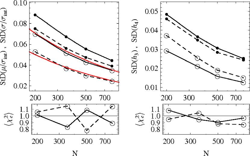
Figure 7: Upper panels: Accuracy limits from limited sampling with the maximum likelihood method (empty circles). The standard deviation of estimated (normalized) mean $\mu$ (full line) and dispersion $\sigma$ (dashed line) on the left; the standard deviation of the Gauss-Hermite moments $h_{3}$ (full line) and $h_{4}$ (dashed line) on the right. Lower panel: the precision test on the measurements obtained through the maximum likelihood method; coding as in the upper panels.

3.3 Tests of Accuracy and Precision

To evaluate the performance of the maximum likelihood approach, we test its accuracy and precision, in a similar manner to Sect. 2.1 for the Gauss-Hermite series. In order to establish a direct comparison, we use as an intrinsic distribution of the synthetic datasets a perfect Gaussian $\mathscr{L}(v)=\mathscr{G}(\mu_{\rm int},\sigma_{\rm int})$. Also, we convert ${s}$ and ${a}$ into measurements of $h_{3}$ and $h_{4}$ by using the transformations (20). All measurements are obtained by using a Metropolis-Hastings procedure, which allows us to scan efficiently the 4-dimensional parameter space defined by our parametrization.

Our results are collected in Fig. 7. The upper panels display the accuracy test, and are analogous to the panels of Fig. 1. The results obtained for the maximum likelihood method are denoted by empty circles. It is evident that both StD$(\mu)$ and StD$(\sigma)$ follow very closely their respective statistical prescriptions ($1/\sqrt{N}$ and $1/\sqrt{2N}$, in red). Hence, the method achieves the maximum measuring power allowed by the sample size. As for the deviations from Gaussianity, both StD$(h_{3})$ and StD$(h_{4})$ are substantially smaller than in the binned case of Sect. 2.1. Experiments with non-Gaussian intrinsic velocity distributions show an even smaller shot noise, athough with qualitatively similar figures. The relative gain in accuracy for the detections of symmetric deviations is found to be an increasing function of the sample size, reaching approximately 2 for $N=800$ and surpassing 2 for asymmetric deviations. These quantities refer to the idealized case of datasets with no observational uncertainty ($\delta_{i}=0$) and uniform certainty of membership ($p_{i}=1$). Hence, they represent only lower bounds for the actual gains that are achievable in any real case.

Lower panels display the precision test, which evaluates the reliability of the uncertainties returned by the maximum likelihood procedure. The $\langle\chi^{2}_{e}\rangle$ quantity in the plots represents the average (over the number of performed tests) for the quantity

$$\chi^{2}_{e}=\left({{\theta-\theta_{\rm int}}\over{e_{\theta}}}\right)^{2}\ ,$$ (21)

where $\theta$ stands for any parameter of the family of distributions and $\theta_{\rm int}$ is its intrinsic, input value. We recall that $e_{\theta}$ denotes the uncertainty on the measured value of the parameter as returned by the marginalized likelihood. We find that the errors on $\mu$ and $\sigma$, as well as those on $s$ and $a$ behave as desired, with all $\langle\chi^{2}_{e}\rangle$ averaging approximately to the expected value of unity.

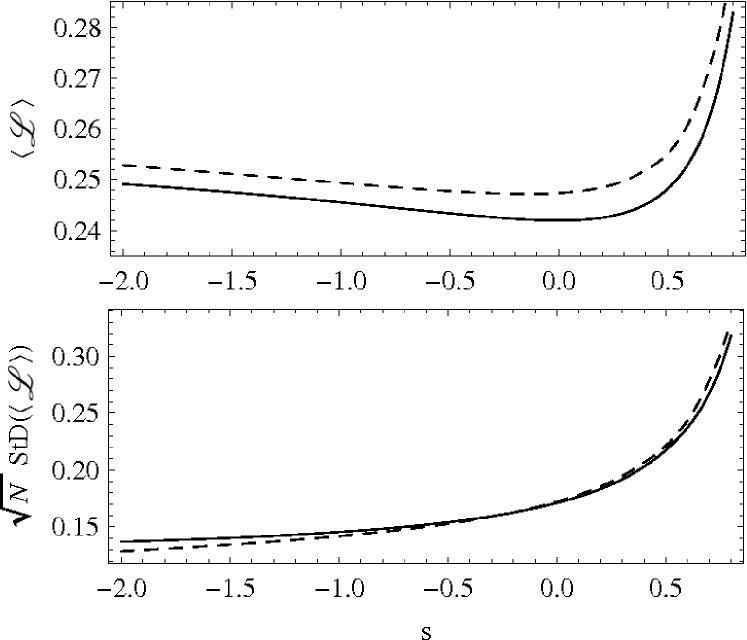
Figure 8: The average $\langle\mathscr{L}\rangle$ (upper panel) and standard deviation StD$(\langle\mathscr{L}\rangle)$ (lower panel) for different symmetric deviations $s$. In both panels, full lines represent the case $(s,a=0)$, while dashed lines are $(s,|a|=0.5)$.

3.4 A Check on the Degree of Flexibility

It is natural to raise the question: what if the intrinsic distribution is not included in our two-parameter family? This may represent the greatest disadvantage of the maximum likelihood implementation, because for extremely high sample sizes and observational precision of kinematic measurements, the standard Gauss-Hermite expansion can be made as flexible as necessary by adding higher order terms. However, it is possible to set up an efficient device that controls whether the family of distributions is appropriate and flexible enough.

For the Gauss-Hermite series, this device is represented by Myller-Lebedeff’s theorem, which equates the integral of the residuals between the observed distribution and its best Gaussian fit with the sum of the Gauss-Hermite moments themselves (eqns (12-14) in van der Marel & Franx (1993)). This allows us to check whether the adopted truncation of the Gauss-Hermite series is completely satisfactory, and if further higher order terms are required.

Within our maximum likelihood approach, it is necessary to ask a more purely statistical question: given the observed sample $\vec{V}$ (which comes together with the associated uncertainties $\vec{\Delta}$, the membership probabilities $\vec{P}$, and its sample size $N$) and the distribution $\mathscr{L}$ that – within the considered family – provides the maximum likelihood, would an analogous sample, actually extracted from the same $\mathscr{L}$, be fitted significantly better? It is possible to answer this question quite easily in an analytic way.

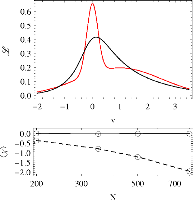
Figure 9: A test of our statistical device. Upper panel: the input distribution in red and its best description within our family in black. Lower panel: evolution with the sample size of the average (on the series of tests) of the $\chi$ quantity defined in eqn (26). Dashed line: the synthetic datasets are distributed according to the red input distribution shown in the upper panel; full line: the synthetic datasets are distributed according to the black best-fit distribution shown in the upper panel.

Let us suppose that $\vec{\Theta}$ is the set of parameters that provides the maximum likelihood for the sample $\vec{V}$, accompanied by $\vec{\Delta}$ and $\vec{P}$:

$$L(\vec{\Theta})=\prod_{i=1}^{N}p_{i}\ \left[\mathscr{L}\ast\mathscr{G}(0,\delta_{i})\right](v_{i})\ .$$ (22)

The value of $L(\vec{\Theta})$ can be compared with the characteristic value of the analogous product in eqn (22) in which the velocities $v_{i}$ are actually extracted from the distribution given by the set of $\vec{\Theta}$:

$$\langle L(\vec{\Theta})\rangle=\langle\prod_{i=1}^{N}p_{i}\ \mathscr{L}\ast\mathscr{G}\rangle=\prod_{i=1}^{N}p_{i}\ \int\left[\mathscr{L}\ast\mathscr{G}(0,\delta_{i})\right]^{2}\ .$$ (23)

Since both quantities defined by eqns (22) and (23) converge to zero quickly with $N$, we find it more convenient to consider their nonvanishing counterparts $\sqrt[N]{L(\vec{\Theta})}$ and $\langle\sqrt[N]{L(\vec{\Theta})}\rangle$. In order to ease the notation, we use the simplification

$$\left\{\begin{array}[]{rcl}\langle\sqrt[N]{L(\vec{\Theta})}\rangle&=&\langle L\rangle\\ \sqrt[N]{L(\vec{\Theta})}&=&\bar{L}\end{array}\right.\ .$$ (24)

If the distance between $\bar{L}$ and $\langle L\rangle$ can be accounted for by the natural scatter introduced by the sample size $N$ only, then the distribution given by the set $\vec{\Theta}$ provides a statistically perfect description of the sample $\vec{V}$. This natural scatter is clearly given by

$${\rm StD}\left[\langle L\rangle\right]=\sqrt{\langle{L(\vec{\Theta})^{2/N}}\rangle-\langle L\rangle^{2}}\ ,$$ (25)

hence the quantity we are interested in is

$$\chi={{\left(\bar{L}-\langle L\rangle\right)}/{{\rm StD}\left[\langle L\rangle\right]}}\ .$$ (26)

Values of $\chi^{2}$ up to unity indicate that the sample $\vec{V}$ is statistically well described. Negative values of $\chi$, with absolute value significantly larger than unity, indicate that the adopted parametrization is not able to provide a good statistical description of the sample.

To apply this criterion, we need explicit expressions for both $\langle L\rangle$ and ${\rm StD}\left[\langle L\rangle\right]$. It is useful to note that for a fixed set of parameters $\vec{\Theta}$, both $\langle L\rangle$ and ${\rm StD}\left[\langle L\rangle\right]$ are invariant with respect to a change in $\mu$, which we can ignore. Also, if we indicate with $\langle L(\sigma=1,\vec{\Theta}_{\rm sh})^{1/N}\rangle$ and ${\rm StD}\left[\langle L(\sigma=1,\vec{\Theta}_{\rm sh})^{1/N}\rangle\right]$, the values attained for $\sigma=1$ (all others $\theta_{j}$, $\vec{\Delta}$ and $\vec{P}$ fixed), then for a general $\sigma$ it is easy to verify that

$$\langle L(\sigma,\vec{\Theta}_{\rm sh})^{1/N}\rangle = \langle L(\sigma=1,\vec{\Theta}_{\rm sh})^{1/N}\rangle\big{/}\sigma$$ (27)

$${\rm StD}\left[\langle L(\sigma,\vec{\Theta}_{\rm sh})^{1/N}\rangle\right] = {\rm StD}\left[\langle L(\sigma=1,\vec{\Theta}_{\rm sh})^{1/N}\rangle\right]\big{/}\sigma\ ,$$

where the uncertainties are scaled accordingly, i.e., $\delta_{i}\rightarrow\delta_{i}/\sigma$. As a consequence, we can restrict the problem to the case $\sigma=1$.

We use now the fact that, for large $N$, the different convolutions can be accounted for by the mean $\delta_{m}$ of the sample of uncertainties $\vec{\Delta}$, and after some algebra, we find the following asymptotic expressions, valid for the case $\sigma=1$:

$$\langle L\rangle = \prod_{i}p_{i}^{1/N}\int\left[\mathscr{L}\ast\mathscr{G}(0,\delta_{m}/\sigma)\right]^{1+1/N}$$ (28)

$$= p_{\rm gm}\ \exp(A)+O(1/N)$$

$${\rm StD}\left[\langle L\rangle\right] = \left\{\prod_{i}p_{i}^{2/N}\int\left[\mathscr{L}\ast\mathscr{G}(0,\delta_{m}/\sigma)\right]^{1+2/N}-\langle L\rangle^{2}\right\}^{1/2}$$ (29)

$$= p_{\rm gm}\ \exp(A)\sqrt{B-A^{2}}/\sqrt{N}+O(1/N)$$

in which $p_{\rm gm}$ is the geometric mean of the sample’s membership probabilities $\vec{P}$

$$p_{\rm gm}=\sqrt[N]{\prod_{i=1}^{N}p_{i}}$$ (30)

and $A$ and $B$ are the following simple integrals (we implicitly assume that $\mathscr{G}=\mathscr{G}(0,\delta_{m}/\sigma)$)

$$A=A(\sigma=1,\vec{\Theta}_{\rm sh}) = \int(\mathscr{L}\ast\mathscr{G})\log\left(\mathscr{L}\ast\mathscr{G}\right)$$ (31)

$$B=B(\sigma=1,\vec{\Theta}_{\rm sh}) = \int(\mathscr{L}\ast\mathscr{G})\log\left(\mathscr{L}\ast\mathscr{G}\right)^{2}\ .$$ (32)

Eqns. (28 - 32) allow us to compute directly, for any value of the parameters $\theta_{j}$, all necessary ingredients to compute $\chi$ in eqn (26), and hence to understand whether the fit of the observed sample is indeed statistically good.

As a reference and an example, we consider here the simplified case in which there is no observational uncertainty, $\delta_{m}=0$, and the likelihood is maximized by the distribution $\mathscr{L}$, having dispersion $\sigma=1$. With a slight abuse of notation, we use $\langle\mathscr{L}\rangle$ to indicate the average of the likelihood in the sense of eqn (23) and ${\rm StD}(\langle\mathscr{L}\rangle)$ to indicate its standard deviation, as in eqn (25). For the Gaussian case, $\mathscr{L}=\mathscr{G}(\mu,\sigma=1)$, both integrals $A$ and $B$ are analytic and we find

$$\begin{array}[]{rcccl}\langle\mathscr{G}\rangle&=&1\big{/}\sqrt{2\pi e}&\approx&0.24197\ ;\\ \sqrt{N}\ {\rm StD}(\langle\mathscr{G}\rangle)&=&1\big{/}\sqrt{4\pi e}&\approx&0.1711\ .\end{array}$$ (33)

Deviations in $\mathscr{L}$ from the Gaussian profile determine deviations in the average $\langle\mathscr{L}\rangle$ as well as in the corresponding standard deviation ${\rm StD}(\langle\mathscr{L}\rangle)$. Fig. 8 displays the behaviour of $\langle\mathscr{L}\rangle$ and $\sqrt{N}{\rm StD}(\langle\mathscr{L}\rangle)$ for the cases $({s},{a}=0)$ (full line) and $({s},|{a}|=0.5)$ (dashed line). Both the displayed quantities increase significantly for positive values of $s$, due to the change in shape of the associated distributions.

Finally, Figure 9 illustrates a practical test. The distribution in red in the upper panel is used to produce synthetic datasets of different sample sizes, which are then fed to our maximum likelihood formalism. This distribution is not included in our parametric family, and, as a comparison, the distribution in black in the same panel displays its best fit. We perform a large number of tests for different sample sizes and record the evolution of the average of the quantity $\chi$, computed at each test, in the lower panel of the same Figure, as a dashed line. For small sample sizes, it is almost impossible to distinguish the two distributions. Nonetheless, as the sample size increases, the properties of the input distribution become more evident and cannot be completely reproduced within our family, so that $\chi$ reaches a value of $-2$ for $N=800$. The black full line in the lower panel shows, for comparison, the average of the $\chi$ quantity that we obtain for synthetic samples that are drawn directly from the best fit distribution, and that average to the expected value of zero for any sample size.

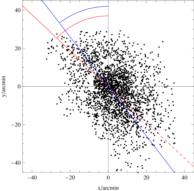
Figure 10: The positional distribution of kinematic measurements in Fornax as from the dataset presented by Walker et al. (2009). The position angle $\theta_{\rm MA}$ is displayed in red, while the apparent rotation axis $\theta_{\rm app}$ (Piatek et al., 2007) is shown in blue.

Figure 11: Results for the Fornax dSph: circular annuli. First row: the symmetric deviations. Second row, left and middle panels: the dispersion. Second row, right panel: the quantity $\chi$ for all displayed maximum likelihood measurements.

Figure 12: Results for the Fornax dSph: angular sectors. Upper panel: datapoints display the mean $\mu$; the black full line shows the prediction for $\mu$ determined by the astrometric measurement of proper motion measured (Piatek et al., 2007) under the assumption of no streaming motion; the red full line displays the correction introduced by intrinsic rotation. Lower panel: the asymmetric deviations.

4 Applications: The Galactic dSphs

4.1 Fornax

The kinematic sample presented by Walker et al. (2009) consists of 2409 measurements for stars with a probability of membership higher than 0.9. We include this information in our likelihood (5), and we discard measurements with a smaller membership probability. As already found in Section 2.2, this kinematic sample comes with a (normalized) level of uncertainty of $\delta_{m}/\sigma\approx 0.22$, which is the smallest in the currently available selection of dSphs. To construct our set of observables, we transform the coordinates of the stars in the plane of the sky with

$$x_{i} = -c\ \cos\delta_{i}\ \sin(\alpha_{i}-\alpha_{0})$$ (34)

$$y_{i} = c\ \left[\sin\delta_{i}\cos\delta_{0}-\cos\delta_{i}\sin\delta_{0}\cos(\alpha_{i}-\alpha_{0})\right],$$ (35)

in which $c$ is a constant ($=10800/\pi$ for coordinates in arcminutes). We adopt the coordinates (J2000) of Fornax’s center as in Mateo (1998), $(\alpha_{0},\delta_{0})=(2^{h}39^{m}59^{s},-34^{\circ}27.0^{\prime})$. The photometric ellipticity ($e=0.30$) and the major axis position angle ($\theta_{\rm MA}=46.8^{\circ}$) are taken from (Battaglia et al., 2006). Fig. 10 shows the resulting spatial distribution of the kinematic measurements on the plane of the sky, with the angle $\theta_{\rm MA}$ highlighted in red.

4.1.1 Symmetric deviations

Given the number of available kinematic measurements and the results of our accuracy tests, we consider a set of different subsample sizes for our measurements: $N\in\{350,500,800\}$. We experimented with both circular and elliptical annuli, but we have found no significant difference, and hence report results for the circular annuli only. For a comparison, we also consider results for minor axis and a major axis regions. Each of these is defined as the sum of the two opposite Cartesian quadrants centered on the relevant axis. Given the smaller number of stars in each of these regions, only $N\in\{350,500\}$ were considered. As we demonstrated in Sect. 2.3, our measurements of the line profiles in circular annuli are not affected by apparent rotation.

Results for symmetric deviations $s$ and velocity dispersion $\sigma$ are displayed in the upper and lower panels of Fig 11. In both rows, the left panels (in shades of grey) illustrate the results for circular annuli, while middle panels show the division according to the major and minor axes regions (respectively, in shades of blue and red). Different shades of the same colour, and different sizes of the corresponding datapoint, are used to indicate the sample size used for each measurement, with larger sizes associated to darker and larger datapoints. The upper-right panel translates the symmetric deviations in terms of the Gauss Hermite coefficient $h_{4}$. The lower-right panel displays the value of the quantity $\chi$ corresponding to each single maximum likelihood measurement.

The symmetric deviations display a clear evolution from positive values of $s$ (and $h_{4}$) in the center of Fornax, to negative values of $s$ (and $h_{4}$) at larger radii, with a tentative return towards a more Gaussian profile at the end of the sample‘s radial coverage ($\approx 3$ half-light radii). The major and minor axes regions show some differences and the minor axis region displays a stronger (negative) signal for $s$. This may perhaps be consistent with an elliptical kinematic pattern following the isophotes. Nonetheless it is interesting to notice that most of the signal for flat-topped distributions is indeed coming from the minor axis region. We confirm a mildly declining dispersion profile in Fornax and also note a systematic difference between the major axis and minor axis regions, with the minor axis showing a lower line of sight velocity dispersion.

If we were to interpret the result by following the suggestions of both Gerhard (1993) and van der Marel & Franx (1993), we would conclude that Fornax shows some degree of tangential anisotropy, at least outside its central regions. We notice that the tentative ‘peak’ of positive values of $s$ (and $h_{4}$) in the very centre may be interpreted in different, possibly non exclusive, ways. The first interpretation invokes the ‘complementarity property’, recognized by Dejonghe (1987): a tangentially biased structure has flat-topped ($s<0$) distributions outside some transition radius and a more spiky ($s<0$) distribution in the central regions. The second interpretation is the existence of two populations with distinct kinematic properties. It is easy to see that the superposition of two approximate Gaussians with different widths would be recognized as a distribution with a positive $s$ – the exact value of which is dependent on both the ratio of numbers and dispersions of the two superposing populations. Finally, there may be place to accommodate a central intermediate mass black hole (IMBH). In this respect, it would be interesting to compare detailed modelling of our results with the constraints obtained by Jardel & Gebhardt (2012) for the IMBH’s mass. Regarding the issue of multiple stellar populations, we also note a systematic tendency of measurements in the inner parts of the system to have higher values of $\chi$. This is consistent with the fact that while at larger radii we are effectively modelling just the metal poor stellar population, towards the center we register the effects coming from two superposing populations.

We do not report explicit results for the asymmetric deviations $a$ or for the mean $\mu$ for circular annuli. Unlike symmetric deviations, asymmetric deviations average to zero over circular annuli. Our results confirm this expectation and we prefer to address the characterization of asymmetric deviations by considering a purely angular subdivision of the dataset, using angular sectors that make no reference to the distance from the centre.

4.1.2 Asymmetric deviations and apparent rotation

In the Fornax dSph, the astrometrically derived proper motion (Piatek et al., 2007) agrees at approximately 1-sigma with the proper motion deduced using the kinematic data under the assumption of no streaming motions (Walker et al., 2008). This testifies to the fact that, if any intrinsic rotation is present, it must be small by comparison with the velocity field given by the apparent rotation. However, a precise measurement for both proper motion and rotation in dSphs is relevant for comparison with simulations, and for constraining the formation history of such systems. For this reason, we reconsider this issue here, and note that our ability to measure asymmetries in the line of sight profiles can help us constrain the intrinsic rotation field. This is because, in the plane of the sky, asymmetries and intrinsic rotational velocities are likely to be strongly correlated.

In the lower panel of Fig. 12, we measure the the ”asymmetry field” in angular sectors $a(\theta)$ around Fornax’s center (on subsamples $N=400$). Although almost everyhere nearly zero, we do detect a $2\pi$-periodic signal, which is indeed compatible with an intrinsic rotation. Not all datapoints in the panel are independent, and hence we do not try to fit our result, but it is encouraging that the peaks of the signal are approximately aligned with the major axis of the system, which is displayed as red vertical lines, $\theta_{\rm peak}\approx\theta_{\rm MA}$. This signal is not due to apparent rotation, and is robust against subtraction of the apparent rotation field.

The datapoints in the upper panel of Fig. 12 show the associated mean in angular sectors $\mu(\theta)$ (on subsamples N=350). This can be compared with the black full line in the same panel, which displays the apparent rotation that the astrometrically derived proper motion implies on the 2-dimensional distribution of kinematic measurements. It is clear that any disagreement is again correlated with the position of the major axis, and has opposite signs in opposite directions, in a way that is compatible with intrinsic rotation. Unfortunately, despite the quality of the dataset, it is not possible to derive a statistically meaningful characterization of the two dimensional intrinsic velocity field. This implies, approximately, an intrinsic rotation of about 1 kms^-1 for the outermost tracers aligned with the major axis in either directions.

Figure 13: The distribution of kinematic measurements in Sculptor as from the dataset presented by Walker et al. (2009) (in black) and from the dataset presented by Starkenburg et al. (2010) in green. The position angle $\theta_{\rm MA}$ is displayed in red.

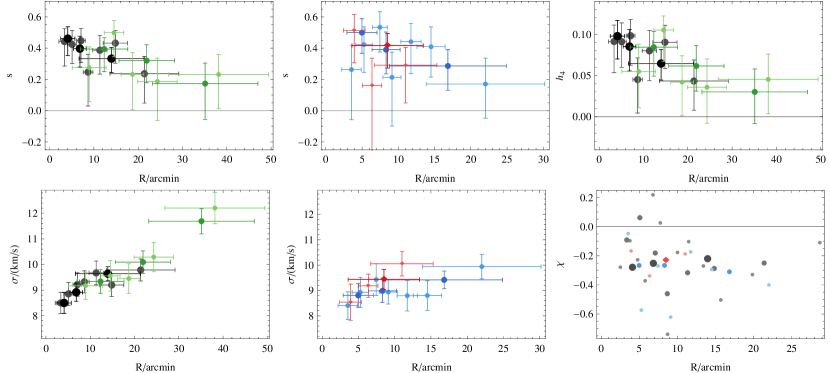
Figure 14: Results for the Sculptor dSph: circular annuli. First row: the symmetric deviations. Second row, left and middle panels: the dispersion. Second row, right panel: the quantity $\chi$ for all displayed maximum likelihood measurements.

Figure 15: Results for the Sculptor dSph: angular sectors. Upper panel: datapoints display the mean $\mu$; full lines show the prediction for the mean $\mu$ determined by the astrometric measurement of proper motion measured (Piatek et al., 2006) and no intrinsic rotation (systematic velocities as from the datasamples). Lower panel: the asymmetric deviations.

4.2 Sculptor

The available sample from Walker et al. (2009) contains 1370 line of sight velocity measurements with membership probability higher than 0.5. We adopt the coordinates (J2000) of the dSph‘s centre from Mateo (1998): $(\alpha_{0},\delta_{0})=(1^{h}00^{m}09^{s},-33^{\circ}42.5^{\prime})$. The photometric ellipticity $e=0.26\pm 0.01$ and position angle $\theta_{\rm MA}=-85.3^{\circ}\pm 0.9^{\circ}$ are taken from de Boer et al. (2011). As reported in Section 2.2, this kinematic sample comes with a (normalized) level of uncertainty of $\delta_{m}/\sigma\approx 0.325$. We accompany this kinematic sample with the one provided by Battaglia et al. (2008) and then recalibrated by Starkenburg et al. (2010) (results related with this datasets are displayed in green in all relevant Figures). To avoid misalignment between the catalogs, for this second dataset we use the dSph center as determined in de Boer et al. (2011). Even though the number of line of sight velocity measurements is lower with 629 giants, they cover a significantly more extended radial region (see Fig 13), which makes the two datasets complementary. Also, a smaller (normalized) level of uncertainty $\delta_{m}/\sigma\approx 0.17$ is achieved.

Given the reduced number of kinematic tracers in comparison to Fornax, we are forced to consider smaller sample sizes: $N\in\{350,500\}$ for the circular annuli and $N\in\{200,350\}$ for the major axis and minor axis regions. Results for symmetric deviations $s$ and velocity dispersion $\sigma$ are displayed respectively in the upper and lower panels of Fig 14. The collected results refer to circular annuli, and again no significant differences were found for the case of elliptical annuli.

The symmetric deviations display a marked preference for positive values of $s$ (and $h_{4}$) for the entire radial range covered by the tracers. This behaviour is confirmed by both datasets, which are found in perfect agreement. Identical profiles (within the uncertainties) are found for the major axis and minor axis regions. Taken at face value, these results support a radially biased dynamical structure, which was also the result of Amorisco & Evans (2012). The central peak in $s$ as well as the tendency for higher values of $\chi$ towards the center mimic the case of Fornax, and hence point towards the effect of superposing populations, even though we cannot exclude other dynamical origins.

We confirm the outwardly increasing velocity dispersion profile in Sculptor, although it should be remembered that the dataset from Battaglia et al. (2008) is not provided with probabilities of membership, hence the outermost points may probably be affected by contamination. Nonetheless, in the radial range where both datasets are available, they agree very well. Surprisingly, we find that the two datasets do not agree in the deduced means $\mu$. The upper panel of Fig. 15 displays the mean in angular sectors $\mu(\theta)$. We detect very similar angular behaviour, but the two datasets seem to be shifted uniformly of about 1 kms^-1. Given that higher order moments all agree, we suspect that such a significant difference may be systematic in origin. Therefore, particular caution should be used when attempting to merge the two datasets.

Unfortunately, neither of the two datasets displays a conclusive signal for the asymmetric deviations (see lower panel in Fig. 15), which does not allow us to make progress in the determination of Sculptor‘s proper motion or intrinsic rotation. It is known that the astrometric measurement of Sculptor‘s proper motion (Piatek et al., 2006) does not agree with the kinematic rotation signal. This suggest either the presence of significant intrinsic rotation or perhaps an error in the astrometric measurement, and is exemplified by the disagreement between the datapoints and the full curves in the upper panel of Fig. 15. Such curves, display the apparent rotation implied by Piatek’s proper motion, and have been normalized to the systematic velocity derived separately by each dataset. In turn, even though roughly agreeing on its direction and qualitatively with the rotation identified in Battaglia et al. (2008), the two kinematic samples would suggest proper motions of different magnitudes, hence further observational effort will be necessary for progress.

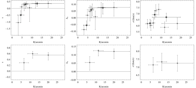
Figure 16: Results for the Carina (upper panels) and the Sextans (lower panels) dSphs. Left and middle panels in both rows: results for the asymmetric deviations. Right panels: velocity dispersion.

4.3 Carina and Sextans

The sizes of the kinematic samples regarding the Sextans and Carina dSphs are significantly smaller than the two previous cases, respectively with 449 and 780 stars with membership probability higher than 0.5 (424 and 758 higher than 0.9). Also, since the intrinsic line of sight velocity dispersion is smaller than in Fornax and Sculptor, the average level of uncertainty goes up, as reported in eqns (2.2). Since the apparent velocity fields are poorly constrained, we decide to avoid their subtraction. For completeness, we use the coordinates of the centers of these dSphs as listed in Mateo (1998). We use, respectively for Sextans and Carina, sample sizes of $N=200$ and $N\in\{175,325\}$.

Results for the symmetric deviations in circular annuli for both dSphs are shown in Fig. 16. Both systems show a tendency (outside the innermost regions in the case of Carina) for line of sight distributions that are more peaked than Gaussian, which is compatible with a radial bias in their orbital structure.

5 Conclusions

We have devised an efficient method to extract the shape information for line profiles of discrete kinematic data. Such information is often crucial in constraining the orbital structure of stellar systems. Independent knowledge of the orbital anisotropy is necessary to break the mass-anisotropy degeneracy, and hence to constrain the mass density profile. Clear-cut determination of the mass profile at both very small and large radii is made challenging by such degeneracies, but nonetheless provides a crucial test for our picture of galaxy formation. Also, the orbital structure retains memory of the initial conditions in which the tracers were formed, and so constrains albeit indirectly the different galaxy formation mechanisms.

Our methods are complementary to the standard Gauss-Hermite formalism, that is best suited for continuous data obtained from absorption line spectra. Discrete kinematic measurements are affected by inhomogeneous uncertainties and often come with varied probabilities of membership. The Gauss-Hermite formalism is unable to account for all this different information, in contrast to a Bayesian approach, which also allows us to avoid any binning procedure.

Since the Gauss-Hermite series is not positive definite, it cannot be used as a probability distributions. Instead, we construct a new family of line profiles derived from velocity distributions and use them in the context of Bayesian inference. Our family has two parameters, namely $s$ which quantifies symmetric deviations from the Gaussian profile and $a$ which refers to the asymmetric deviations. The parameter $s$ has a kinematic interpretation, and is associated with line profiles that mimic those of constant anisotropy models (with an exponential dependence on the energy).

Our methods allow us to measure directly the intrinsic line profiles $\mathscr{L}$, rather than the profile convolved with the observational uncertainties. The advantage of such an approach is substantial. Any signal of a deviation from Gaussianity is significantly stronger in the intrinsic line profile. Hence, a smaller sample size is sufficient to reach the level at which signal itself is larger than the shot noise. We quantify the magnitude of this noise as a function of the sample size and find that, within the Gauss-Hermite formalism, this noise is higher than the expected signal in both $h_{3}$ and $h_{4}$ for sample sizes smaller than N$\approx$200. This casts doubts on measurements obtained on significantly smaller sample sizes, especially if important observational uncertainties are present. We find that our maximum likelihood methods perform in comparison systematically better. Even in the case of zero uncertainties, we achieve a relative gain in accuracy that is about 2 on $h_{4}$ (for sample sizes $N=800$) and higher for $h_{3}$. These quantities cannot but improve in presence of observational uncertainties and estimates for the probabilities of membership.

To ensure that our methods can give reliable descriptions of the shape, we present a simple test that is able to assess the statistical quality of the fit. This is obtained by quantifying the scatter that limited sampling implies on the average value of the likelihood, which can be done analytically. We apply this test to a practical example and confirm that it is indeed able to identify cases in which the adopted family of line profile is not able to provide a good statistical representation of the data.

We apply our formalism to the discrete velocity datasets of the dwarf spheroidals of the Milky Way. We quantify the effects of apparent rotation due to systematic proper motions and find that these are not an issue for the dSphs. We measure detailed radial profiles for the symmetric deviations in Fornax, Sculptor, Carina and Sextans. All systems but Fornax are characterized by line of sight profiles that are substantially more peaked than Gaussian outside the centre. If interpreted following both Gerhard (1993) and van der Marel & Franx (1993), this suggests a radially biased orbital structure in Sculptor, Carina and Sextans. Detailed dynamical modelling is required in order to quantify the orbital structure, and to assess the effects of the stellar density distribution as well as those of the unknown inclination. Nonetheless, on a qualitative level, the sharply falling photometric profile of the dSphs assures us that a significantly peaked velocity dispersion can be robustly associated with a radial bias of the orbits. On the other hand, Fornax, shows line profiles that are flat-topped at large radii, hence perhaps favouring some tangential anisotropy. This suggests that it may have had a different recent accretion history to the other dSphs. Support for this viewpoint is also provided by its distinctive shell structures (e.g., Coleman et al., 2005; Olszewski et al., 2006; Coleman & de Jong, 2008).

We also consider the angular behaviour of the asymmetric deviations from Gaussianity. In Fornax, we find a systematic angular trend, that we interpret as originating in a small level of intrinsic rotation. In fact, we find that this trend is mirrored in systematic residuals in the mean velocity with respect to the astrometrically determined proper motion. This is consistent with a mild intrinsic rotation about the minor axis, reaching about 1 kms^-1 in the radial range covered by the kinematic sample.

Our methods for characterizing the shapes of line profiles in discrete kinematic datasets are both powerful and adaptable. In recent times, the size and variety of such datasets has increased substantially, with applications that range from the kinematics of the globular cluster populations in relatively distant massive galaxies to precision kinematics of giant stars in our own Galactic neighborhood. We anticipate that our methods will find ready application to a rich variety of datasets, and are actively pursuing further applications.

Appendix A Construction of asymmetric deviations

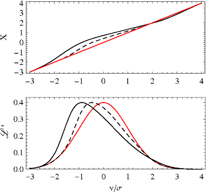
Figure 17: The construction of asymmetric distributions. The upper panel displays the comparison between the identity function ${\rm X}({s},{a}=0;v)$ (in red) and two analogous functions (with ${s}=0$) obtained for nonzero values of a (respectively ${a}=0.3$ as a dashed line and ${a}=0.6$ as a dashed line). The lower panel illustrates, with the same graphical coding, the associated distributions $\mathscr{L}^{\prime}$, constructed as in eqn (17).

We considered several alternatives for the implementation of asymmetric deviations starting with a simple parametrization compatible with the general form

$$f=f_{\rm e}({s})(1-{a}f_{\rm o}({s},{a}))\ ,$$ (36)

where $f_{\rm e}$ and $f_{\rm o}$ are respectively an even and odd function of one of the components of the tangential velocity $\vec{v}_{t}$, for example $v_{\theta}$, and $a$ is the parameter for asymmetric deviations. This approach has not been successful for at least two reasons.

First, the asymmetric deviations produced by the functional form (36) – which has to satisfy the consistency requirement $f\geq 0$ – are too small for our purposes. It is importnat to have a large template of deviations during the measuring procedure. Depending on the sample size and given the natural accuracy limits we quantified in Sect 2.1, even in the case of an intrinsically symmetric distribution, distributions with a large asymmetry ($h_{3}\gtrapprox 0.1$) are needed in order to assess a reliable errorbar. Second, the functional form (36) has the significant limit of correlating symmetric and asymmetric deviations. At fixed $s$, $f_{los}(v_{\parallel}=0)$ is in fact invariant with respect to $a$, anh hence, asymmetric deviations come together with a more spiky profile, which is not a desirable feature.

Our implementation of asymmetries, presented in eqn. (17) is able to overcome both difficulties. Fig. 17 illustrates the main ingredients of this approach. The upper panel displays the comparison between the identity function in red, representing the case ${\rm X}({s},{a}=0;v)$, and two analogous functions obtained for ${s}=0$ but nonzero values of $a$. In the lower panel we display the associated distributions $\mathscr{L}^{\prime}$, in comparison with the Gaussian profile in red. Our function $X$ in eqn (18) is constructed in order to comply with a series of requirements.

• $X$ is asymptotic to $v$ at both negative and positive extremes of the real axis. This is achieved by the structure $X-v\sim\exp(v^{4})$.

• The choice of the fourth power (rather than the second, for example) assures that asymmetric distributions are not significantly spikier than the associated symmetric distribution: $X$ and $v$ are almost parallel when $X\approx 0$.

• The dependences on ${a}$ in the exponential term are required so to adapt the magnitude of the deviations of $X$ from $v$ to the size of the interval (as well as its position) where these deviations need to affect $\mathscr{L}^{\prime}$.

• $X$ has to cross the identity function in order to guarantee a shallow decline on one of the wings of the asymmetric distribution, that in turn crosses the associated symmetric distribution. This is obtained by the linear term that multiplies the exponential one in $X$.

• This crossing point is adjusted to both the shape of the symmetric distribution and to the magnitude of the asymmetric deviations by the dependences on $s$ and $a$ in the mentioned linear term.

• Finally, the multiplication by $a/|a|$ ensures that the magnitude and shape of asymmetric deviations are identical (other than in direction) for positive and negative values of a.

References

- Amorisco & Evans (2012) Amorisco, N. C., & Evans, N. W. 2012, MN, 419, 184
- Battaglia et al. (2006) Battaglia, G., Tolstoy, E., Helmi, A., et al. 2006, AA, 459, 423
- Battaglia et al. (2008) Battaglia, G., Helmi, A., Tolstoy, E., et al. 2008, ApJL, 681, L13
- Coccato et al. (2009) Coccato, L., Gerhard, O., Arnaboldi, M., et al. 2009, MN, 394, 1249
- Coleman et al. (2005) Coleman, M. G., Da Costa, G. S., Bland-Hawthorn, J., & Freeman, K. C. 2005, AJ, 129, 1443
- Coleman & de Jong (2008) Coleman, M. G., & de Jong, J. T. A. 2008, ApJ, 685, 933
- Deason et al. (2012) Deason A., Belokurov V., Evans N.W., McCarthy I., 2012 ApJ, in press
- Dejonghe (1987) Dejonghe H., 1987, MNRAS, 224, 13
- de Boer et al. (2011) de Boer, T. J. L., Tolstoy, E., Saha, A., et al. 2011, AA, 528, A119
- de Boer et al. (2012) de Boer, T. J. L., Tolstoy, E., Hill, V., et al. 2012, AA, 539, A103
- Evans (1994) Evans, N. W. 1994, MN, 267, 333
- Evans et al. (2009) Evans, N. W., An, J., & Walker, M. G. 2009, MN, 393, L50
- Feast et al. (1961) Feast, M. W., Thackeray, A. D., & Wesselink, A. J. 1961, MN, 122, 433
- Gerhard (1991) Gerhard, O. E. 1991, MN, 250, 812
- Gerhard (1993) Gerhard, O. E. 1993, MN, 265, 213
- Gilmore et al. (2007) Gilmore, G., Wilkinson, M. I., Wyse, R. F. G., Kleyna, J. T., Koch, A., Evans, N. W., & Grebel, E. K. 2007, ApJ, 663, 948
- Jardel & Gebhardt (2012) Jardel, J., & Gebhardt, K. 2012, ApJ, in press, arXiv:1112.0319
- Kleyna et al. (2002) Kleyna, J., Wilkinson, M. I., Evans, N. W., Gilmore, G., & Frayn, C. 2002, MN, 330, 792
- Kleyna et al. (2004) Kleyna, J. T., Wilkinson, M. I., Evans, N. W., & Gilmore, G. 2004, MN, 354, L66
- Koposov et al. (2011) Koposov, S. E., Gilmore, G., Walker, M. G., et al. 2011, ApJ, 736, 146
- Łokas & Mamon (2003) Łokas, E. L., & Mamon, G. A. 2003, MN, 343, 401
- Mateo (1998) Mateo, M. 1998, ARAA, 36, 435
- Napolitano et al. (2011) Napolitano, N. R., Romanowsky, A. J., Capaccioli, M., et al. 2011, MN, 411, 2035
- Olszewski et al. (2006) Olszewski, E. W., Mateo, M., Harris, J., et al. 2006, AJ, 131, 912
- Piatek et al. (2006) Piatek, S., Pryor, C., Bristow, P., et al. 2006, AJ, 131, 1445
- Piatek et al. (2007) Piatek, S., Pryor, C., Bristow, P., et al. 2007, AJ, 133, 818
- Rangwala et al. (2009) Rangwala, N., Williams, T. B., & Stanek, K. Z. 2009, ApJ, 691, 1387
- Reijns et al. (2006) Reijns, R. A. et al. 2006, AA, 445, 503
- Romanowsky et al. (2003) Romanowsky, A. J., Douglas, N. G., Arnaboldi, M., et al. 2003, Science, 301, 1696
- Starkenburg et al. (2010) Starkenburg, E., Hill, V., Tolstoy, E., et al. 2010, AA, 513, A34
- van de Ven et al. (2006) van de Ven, G., van den Bosch, R. C. E., Verolme, E. K., & de Zeeuw, P. T. 2006, AA, 445, 513
- van der Marel & Franx (1993) van der Marel, R. P., & Franx, M. 1993, ApJ, 407, 525
- Walker et al. (2008) Walker, M. G., Mateo, M., & Olszewski, E. W. 2008, ApJL, 688, L75
- Walker et al. (2009) Walker, M. G., Mateo, M., & Olszewski, E. W. 2009, AJ, 137, 3100
- Walker et al. (2010) Walker, M. G., Mateo, M., Olszewski, E. W., Peñarrubia, J., Evans, N.W., & Gilmore, G. 2010, ApJ, 710, 886
- Walker & Peñarrubia (2011) Walker, M. G., & Peñarrubia, J. 2011, ApJ, 742, 20
- Wilkinson et al. (2004) Wilkinson, M. I., Kleyna, J. T., Evans, N. W., Gilmore, G. F., Irwin, M. J., & Grebel, E. K. 2004, ApJL, 611, L21
- Wojtak & Łokas (2010) Wojtak, R., & Łokas, E. L. 2010, MN, 408, 2442