Chapter 2 Theoretical Models of SOC Systems

by Markus J. Aschwanden

How can the universe start with a few types of elementary particles at the big bang, and end up with life, history, economics, and literature? The question is screaming out to be answered but it is seldom even asked. Why did the big bang not form a simple gas of particles, or condense into one big crystal? (Bak 1996). The answer to this fundamental question lies in the tendency of the universal evolution towards complexity, which is a property of many nonlinear energy dissipation processes. Dissipative nonlinear systems generally have a source of free energy, which can be partially dissipated whenever an instability occurs. This triggers an avalanche-like energy dissipation event above some threshold level. Such nonlinear processes are observed in astrophysics, magnetospheric physics, geophysics, material sciences, physical laboratories, human activities (stock market, city sizes, internet, brain activity), and in natural hazards and catastrophes (earthquakes, snow avalanches, forest fires). A tentative list of SOC phenomena with the relevant sources of free energy, the physical driver mechanisms, and instabilities that trigger a SOC event are listed in Table 2.1.

A prominent theory that explains such nonlinear energy dissipation events is the so-called Self-organized criticality (SOC) concept, first pioneered by Bak et al. (1987, 1988) and simulated with cellular automaton models, which mimic next-neighbour interactions leading to complex patterns. The topic of SOC is reviewed in recent reviews, textbooks, and monographs (e.g., Bak 1996; Jensen 1998; Turcotte 1999; Charbonneau et al. 2001; Hergarten 2002; Sornette 2004; Aschwanden 2011a; Crosby 2011; Pruessner 2012). SOC can be considered as a basic physics phenomenon - universally occurring in systems with many coupled degrees of freedom in the limit of infinitesimal external forcing. This theory assumes a critical state that is robust in the sense that it is self-organizing, like a critical slope of a sandpile is maintained under the steady (but random) dropping of new sand grains on top of the pile. Individual avalanches occur with unpredictable sizes, uncorrelated to the disturbances produced by the input. Sandpile avalanches are a paradigm of the SOC theory, which has the following characteristics: (1) Individual events are statistically independent, spatially and temporally (leading to random waiting time distributions); (2) The size or occurrence frequency distribution is scale-free and can be characterized by a powerlaw function over some size range; (3) The detailed spatial and temporal evolution is complex and involves a fractal geometry and stochastically fluctuating (intermittent) time characteristics (sometimes modeled with 1/f-noise, white, pink, red, or black noise).

Table 2.1: Examples of physical processes with SOC behavior.

SOC Phenomenon	Source of free energy	Instability or
	or physical mechanism	trigger of SOC event
Galaxy formation	gravity, rotation	density fluctuations
Star formation	gravity, rotation	gravitational collapse
Blazars	gravity, magnetic field	relativistic jets
Soft gamma ray repeaters	magnetic field	star crust fractures
Pulsar glitches	rotation	Magnus force
Blackhole objects	gravity, rotation	accretion disk instability
Cosmic rays	magnetic field, shocks	particle acceleration
Solar/stellar dynamo	magnetofriction in tachocline	magnetic buoyancy
Solar/stellar flares	magnetic stressing	magnetic reconnection
Nuclear burning	atomic energy	chain reaction
Saturn rings	kinetic energy	collisions
Asteroid belt	kinetic energy	collisions
Lunar craters	lunar gravity	meteroid impact
Magnetospheric substorms	electric currents, solar wind	magnetic reconnection
Earthquakes	continental drift	tectonic slipping
Snow avalanches	gravity	temperature increase
Sandpile avalanches	gravity	super-critical slope
Forest fire	heat capacity of wood	lightening, campfire
Lightening	electrostatic potential	discharge
Traffic collisions	kinetic energy of cars	driver distraction, ice
Stockmarket crash	economic capital, profit	political event, speculation
Lottery win	optimistic buyers	random drawing system

There are some related physical processes that share some of these characteristics, and thus are difficult to discriminate from a SOC process, such as turbulence, Brownian motion, percolation, or chaotic systems (Fig. 2.1, right column). A universal SOC theory that makes quantitative predictions of the powerlaw-like occurrence frequency and waiting time distributions is still lacking. We expect that the analysis of large new databases of space observations and geophysics records (available over at least a half century now) will provide unprecedented statistics of SOC observables (Fig. 2.1, left column), which will constrain the observed and theoretically predicted statistical distribution functions (Fig. 2.2, middle column), and this way confirm or disprove the theoretical predictions of existing SOC theories and models (Fig. 2.2, right column). Ultimately we expect to find a set of observables that allows us to discriminate among different SOC models as well as against other nonlinear dissipative processes (e.g., MHD turbulence). In the following we will describe existing SOC models and SOC-related processes from a theoretical point of view.

Figure 2.1: Metrics of observables, statistical distributions, and physical models that need to be defined in order to discriminate SOC from non-SOC processes.

2.1 Cellular Automaton Models (CA-SOC)

The theoretical models can be subdivided into: (i) a mathematical part that deals with the statistical aspects of complexity, which is universal to all SOC phenomena and essentially “physics-free” (such as the powerlaw-like distribution functions), and (ii) a physical part that links the observable parameters to a particular physical mechanism (for instance in form of scaling law relationships between physical parameters).

2.1.1 Statistical Aspects

The original concept of self-organized criticality was pioneered by Bak et al. (1987, 1988), who used the paradigm of a sandpile with a critical slope to qualitatively illustrate the principle of self-organized criticality. The first theoretical description of the SOC behavior of a nonlinear system was then studied with a large number of coupled pendulums and with numerical experiments that have been dubbed cellular automaton models (CA-SOC). In essence, a SOC system has a large number of elements with coupled degrees of freedom, where a random disturbance causes a complex dynamical spatio-temporal pattern. Although such a nonlinear system obeys classical or quantum-mechanical physics, it cannot be described analytically because of the large number of degrees of freedom. The situation is similar to the N-body problem, which cannot be solved analytically for more complex configurations than a two-body system. However, such SOC systems can easily be simulated with a numerical computer program, which starts with an initial condition defined in a lattice grid, and then iteratively updates the dynamical state of each system node, and this way mimics the dynamical evolution and statistical distribution functions of SOC parameters. Hence, such numerical lattice simulations of SOC behavior (i.e., cellular automatons) were the first viable method to study the SOC phenomenon on a theoretical basis.

What are the ingredients and physical parameters of a cellular automaton model? What is common to all cellular automaton models of the type of Bak, Tang, and Wiesenfeld (1987, 1988), briefly called BTW models, is: (1) A S-dimensional rectangular lattice grid, say a coordinate system $x_{i,j,k},i=1,...,n;j=1,...,n,k=1,...,n$ for a 3-dimensional case $S=3$ with grid size $n$; (2) a place-holder for a physical quantity $z_{i,j,k}$ associated with each cellular node $x_{i,j,k}$, (3) a definition of a critical threshold $z_{crit}$, (4) a random input $\Delta z_{i,j,k}$ in space and time; (5) a mathematical re-distribution rule that is applied when a local physical quantity exceeds the critical threshold value, for instance a critical slope of a sandpile, which adjusts the state of the next-neighbor cells, i.e.,

$$\begin{array}[]{ll}z_{i,j,k}=z_{i,j,k}+1&{\rm initial\ input}\\ z_{i,j,k}=z_{i,j,k}-8&{\rm if}\ z_{i,j,k}\geq 8,\\ z_{i\pm 1,j\pm 1,k\pm 1}=z_{i\pm 1,j\pm 1,k\pm 1}+1&\end{array}$$

for the 8 next neighbors in a 3D-lattice grid, and (6) iterative steps in time to update the system state $z_{i,j,k}(t)$ as a function of time $t$. Such cellular automaton simulations usually start with a stable initial condition (e.g., an empty system with $z_{i,j,k}(t=0)=0$), and have then to run several million time steps before they reach a critical state. Once they reach the critical state, avalanches of arbitrary sizes can be triggered by the random input of an infinitesimal disturbance $\Delta z_{i,j,k}(t)$, separated by quiescent time intervals in between, in the case of slow driving. Statistics of the occurrence frequency distributions of avalanche sizes or durations yields then the ubiquitous powerlaw-like distribution functions. Fig. 2.2 shows an example of a 2D-lattice simulation, displaying a snapshot of a large avalanche (top left panel) as well as the statistical distribution function of avalanche sizes $L$ (left) and durations $T$ (right panels).

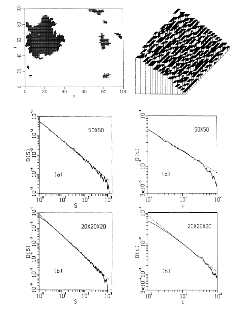
Figure 2.2: Examples of a fragmented avalanche (top left) occurring in a 2-D (computer) sandpile (top right) and occurrence frequency distribution of avalanche cluster sizes (left panels) and avalanche durations (right panels) of the original BTW sandpile cellular automaton simulation. The simulations have been performed for a 50$\times$50 2-D lattice (middle panels) and for a 20$\times$20$\times$20 3-D lattice grid (bottom panels). The powerlaw slopes are $\alpha_{S}=1.0$ and $\alpha_{T}=0.42$ for the 2-D grid (middle panels) and $\alpha_{S}=1.37$ and $\alpha_{T}=0.92$ for the 3-D grid. Reprinted from Bak, Tang, and Wiesenfeld (1987, 1988) with permission; Copyright by American Physical Society.

Thus, such SOC cellular automaton models primarily quantify the spatio-temporal dynamics of complex systems and the related statistics of emerging spatio-temporal patterns. They can predict the distribution function $N(L)dL$ of the size or length scale $L$ of dynamical events (also called “avalanches”), or the time scale $T$ of an avalanche event. Secondary dynamical parameters can be derived, such as the instantaneous avalanche volume $V(t)$ or its change $dV(t)/dt$ during an avalanche event, or the total time-integrated volume of the avalanche $\int_{0}^{T}V(t)dt$. However, such SOC cellular automaton models are “physics-free”, because the dynamics of an event is described by a mathematical rule that substitutes for the unknown physical process, but is thought to be an universal property of SOC systems in a critical state. Applying cellular automaton simulations to observed phenomena requires than to substitute a physical quantity into the “place-holder” variable $z_{i,j,k}$, which is otherwise undefined in cellular automata, except for defining the instability criterion $z_{i,j,k}>z_{crit}$ in terms of a critical threshold $z_{crit}$.

There is a large industry of cellular automaton models, mostly modified versions of the original BTW-model, such as the lattice-gas model (Jensen 1998), Conway’s game of life model (Bak, Chen and Creutz 1989), traffic jam simulations (Nagel and Paczuski 1995), multiple-strategy agent-based models applied to the financial market (Feigenbaum 2003), punctuated equilibrium models applied to biophysics (Bak and Sneppen 1993), slider-block spring models applied in geophysics (Burridge and Knopoff 1967), forest-fire models (Malamud et al. 1998; reviewed in Turcotte 1999), applications to magnetospheric substorms (Takalo et al. 1993; 1999a,b), to solar flares (Lu and Hamilton 1991; Charbonneau et al. 2001), and to stellar accretion disks (Mineshige et al. 1994a,b; Pavlidou et al. 2001). More complete reviews of such cellular automaton models are given in Turcotte (1999) and Aschwanden (2011a, Section 2).

2.1.2 Physical Aspects

Every theoretical model needs verification by experiments and observations. Since a cellular automaton model is a purely mathematical model of complexity, similar to the mathematical definition of a fractal dimension, its predictions of a particular mathematical distribution function (such as a powerlaw) may represents a universal property of SOC processes, but does not represent a complete physical model per se that can be used for applications to real observations. The physical aspect of a SOC model is hidden in the “place-holder” variable $z_{i,j,k}$ and its scaling laws with observables, which require a specific physical mechanism for each observed phenomenon (for examples see second column in Table 2.1).

If we go back to the original SOC concept of avalanches in a sandpile, say in the 1D-version, the place-holder variable $z_{i}$ has been interpreted as a vertical altitude or height difference $z_{i}=h_{i+1}-h_{i}$ between next-neighbor nodes, so that the instability threshold corresponds to a critical slope $z_{i}>z_{crit}=(dh/dx)_{crit}$. For the 3D version, the re-distribution rule is given in Eq. (2.1). The instability threshold essentially corresponds to a critical point where the gravitational force exceeds the frictional force of a sand grain.

In applications to solar flares or magnetospheric substorms, the “place-holder” variable $z_{i,j,k}$ has been related to the magnetic field $B_{i,j,k}=B(x_{i,j,k})$ at location $x_{i,j,k}$, and a related magnetic energy $E_{B}=B^{2}/(8\pi)$ can be defined. The instability criterion $\Delta B>z_{crit}$ involves than a magnetic gradient or magnetic field curvature (Charbonneau et al. 2001),

$$\Delta B=B_{i,j,k}-{1\over 2S}\sum_{nn=1}^{2S}B_{nn}\ ,\qquad|\Delta B|>z_{crit}$$

where the summation includes all $2\times S$ nearest neighbors ($``nn^{\prime\prime}$) in a Cartesian S-dimensional lattice.

More realistically, physics-based models have been attempted by applying the magneto-hydrodynamic (MHD) equations to the lattice field $B({\bf x})$, obeying Ampère’s law for the current density ${\bf j}$,

$${\bf j}={1\over 4\pi}(\nabla\times{\bf B})\ ,$$

which yields together with Ohm’s law the induction equation,

$${\partial{\bf B}\over\partial t}=\nabla\times(\bf v\times{\bf B})+\eta\nabla^{2}{\bf B}\ ,$$

and fulfills the divergence-free condition for the magnetic field,

$$\nabla\cdot{\bf B}=0\ .$$

The instability threshold can then be expressed in terms of a critical resisitivity $\eta$. Such cellular models with discretized magneto-hydrodynamics (MHD) have been applied to magnetospheric phenomena, triggering magnetospheric substorms by perturbations in the solar wind (Takalo et al. 1993; 1999), as well as to solar flares (Vassiliadis et al. 1998; Isliker et al. 1998). Initially, solar flares were modeled with isotropic magnetic field cellular automaton models (Lu and Hamilton 1991). However, since the plasma-$\beta$ parameter is generally smaller than unity in the solar corona, particle and plasma flows are guided by the magnetic field, and thus SOC avalanches are more suitably represented with anisotropic 1D transport (Vlahos et al. 1995). Other incarnations of cellular SOC models mimic the magnetic field braiding that is thought to contribute to coronal heating (Morales and Charbonneau 2008). On the other side, SOC models that involve discretized ideal MHD equations have been criticized to be inadequate to describe the highly resistive and turbulent evolution of magnetic reconnection processes, which are believed to be the driver of solar flares.

Besides the magnetic field approach of the a physical variable in SOC lattice simulations, which predicts the magnetic energy $E_{B}\propto B^{2}/(8\pi)$ or current ${\bf j}\propto\nabla\times{\bf B}$ in each node point, we still have to model the physical units of observables. The magnetic field or electric currents can only be observed by in-situ measurements, which is possible for magnetospheric or heliospheric phenomena with spacecraft, but often observables can only be obtained by remote-sensing measurements in form of photon fluxes emitted in various wavelength ranges, such as for solar or astrophysical sources. This requires physical modeling of the radiation process, a component that has been neglected in most previous literature on SOC phenomena.

If the physical quantity $z_{i,j,k}$ at each cellular node is defined in terms of an energy $e$, the discretized change of the quantity $dz/dt$ corresponds then to a quantized amount of dissipated energy $<\Delta e>$ per node. The instantaneous energy dissipation rate $de/dt=<\Delta e>dV/dt$ of the system scales then with the instantaneous volume change $dV(t)/dt$, while the total amount of dissipated energy during an avalanche event can be computed from the time integral, $E=<\Delta e>\int_{0}^{t}V(t)dt$, assuming that a mean energy quantum $<\Delta e>$ is dissipated per unstable node.

In astrophysical applications, the observed quantity is usually a photon flux, and thus the energy quantity $e=h\nu$ corresponds to the photon energy at frequency $\nu$, while $<\Delta e>=Nh\nu/\Delta t$ is the photon flux of $N$ photons that are radiated in a volume cell $\Delta V$ during a time step $\Delta t$ for a given radiation process. The conversion of the intrinsic energy dissipation rate $de/dt=<\Delta e>(dV/dt)$ (e.g., of magnetic energy $E_{B}$ in a magnetic reconnection process) has then to be related to the amount of emitted photons $<\Delta e>=Nh\nu/\Delta t$ by a physical model of the dissipation process. The physical model of the radiation process may involve a nonlinear scaling between the amount of dissipated energy and the number of emitted photons in a specific wavelength range, which changes the powerlaw slope of the observed distributions of photon fluxes, compared with the predictions of the generic quantity $z_{i,j,k}$ used in SOC cellular automaton simulations.

2.2 Analytical SOC Models

The complexity of the spatio-temporal pattern of a SOC avalanche is produced by a simple mathematical re-distribution rule that defines the next-neighbor interactions on a microscopic level, while the observed structure manifests itself at the macroscopic level. While cellular automaton models operate on the microscopic level of a lattice cell, the complex macroscopic structure cannot be analytically derived from the microscopic states of the nonlinear system. In classical thermodynamics, the macroscopic state of a gas, such as the velocity distribution function of molecules can be derived from the (binomial) probability distribution function of microscopic states. In contrast, nonlinear dissipative systems in the state of self-organized criticality seem to exhibit a higher level of complexity, so that their macroscopic morphology cannot be analytically derived from the microscopic states. Therefore, analytical models can describe the macroscopic SOC parameters only by simplified approximations of the SOC dynamics, which are aimed to be consistent with the observed (powerlaw-like) probability or occurrence frequency distributions. We will describe a few of such analytical models in the following, which make quantitative predictions of the powerlaw slopes and scaling laws between SOC parameters. Such analytical models can then be used for Monte-Carlo simulations of SOC avalanches and be forward-fitted to the observed distributions of SOC parameters.

2.2.1 Exponential-Growth SOC Model (EG-SOC)

SOC avalanches have always a growth phase with nonlinear characteristics, similar to a multiplicative chain-reaction. Mathematically, the simplest function that grows in a multiplicative way is the exponential function with a positive growth rate. It is therefore not surprising that the first analytical models of SOC processes were based on such an exponential growth function (even when they were not called SOC models at the pre-Bak time). The attractive feature for SOC applications is the fact that the simple assumption of an exponential growth curve combined with random durations automatically leads to a powerlaw distribution function, as we will see in the following.

The earliest analytical models in terms of an exponential growth phase with saturation after a random time interval go back to Willis and Yule (1922) who applied it to geographical distributions of plants and animals. Yule’s model was applied to cosmic rays (Fermi 1949), to cosmic transients and solar flares (Rosner and Vaiana 1978; Aschwanden et al. 1998), to the growth dynamics of the world-wide web (Huberman and Adamic 1999), as well as to the distribution of the sizes of incomes, cities, internet files, biological taxa, and in gene family and protein family frequencies (Reed and Hughes 2002).

Figure 2.3: Time evolution of energy release rate $W(t)$ for 3 different ratios of growth times to saturation times, $\tau_{G}/t_{S}=(0.5,1.0,2.0)$ (left) and the corresponding powerlaw distributions of the peak energy release rate $P$. Note that the event set with the shortest growth time ($\tau_{G}/t_{S}=0.5$) reaches the highest energies and thus produces the flattest powerlaw slope ($\alpha=1+\tau_{G}/t_{S}=1.5$).

Here we describe the analytical derivation of the exponential-growth SOC model, following Aschwanden (2011a, Section 3.1). We define the time evolution of the energy release rate $W(t)$ of a nonlinear process that starts at a threshold energy of $W_{0}$ by

$$W(t)=W_{0}\ \exp{\left({t\over{\tau}_{G}}\right)}\ ,\qquad 0\leq t\leq\tau\ ,$$

where ${\tau}_{G}$ represents the exponential growth time. The process grows exponentially until it saturates at time $t=\tau$ with a saturation energy $W_{S}$,

$$W_{S}=W(t=\tau)=W_{0}\ \exp{\left({\tau\over{\tau}_{G}}\right)}\ .$$

We define a peak energy release rate $P$ that represents the maximum energy release rate $W_{S}$, after subtraction of the threshold energy $W_{0}$, that corresponds to the steady-state energy level before the nonlinear growth phase,

$$P=W_{S}-W_{0}=W_{0}\left[\exp{\left({\tau\over\tau_{G}}\right)}-1\right]\ .$$

In the following, we will refer to the peak energy release rate $P$ also briefly as “peak energy”. For the saturation times $\tau$, which we also call “rise times”, we assume a random probability distribution, approximated by an exponential function $N(\tau)$ with e-folding time constant $t_{S}$,

$$N(\tau)d\tau={N_{0}\over t_{S}}\exp{\left(-{\tau\over t_{S}}\right)}d\tau\ .$$

This probability distribution is normalized to the total number of $N_{0}$ events.

In order to derive the probability distribution $N(P)$ of peak energy release rates $P$, we have to substitute the variable of the peak energy, $P$, into the function of the rise time $\tau(P)$, which yields (using the functional relationship $\tau(P)$ from Eq. 2.8),

$$N(P)dP=N(\tau)d\tau=N[\tau(P)]\left|{d\tau\over dP}\right|dP={N_{0}(\alpha_{P}-1)\over W_{0}}\left({P\over W_{0}}+1\right)^{-\alpha_{P}}\ dP\ ,$$

which is an exact powerlaw distribution for large peak energies ($P\gg W_{0}$) with a powerlaw slope $\alpha_{P}$ of

$$\alpha_{P}=\left(1+{\tau_{G}\over t_{S}}\right)\ .$$

The powerlaw slope thus depends on the ratio of the growth time to the e-folding saturation time, which is essentially the average number of growth times. Examples of time series with avalanches of different growth times ($\tau_{G}/t_{S}=0.5,1.0,2.0$) are shown in Fig. 2.3, along with the corresponding powerlaw distributions of peak energies $P$. Note that the fastest growing events produce the flattest powerlaw distribution of peak energies.

Figure 2.4: Schematic of the time evolution of an avalanche event, consisting of (i) a rise time ($\tau$) with exponential growth of the energy release $W(t)$ from a threshold level $W_{0}$ to the saturation level $W_{S}$, and (ii) a decay time ($D$) with a constant decay rate $\eta=dW/dt=W_{0}/\tau_{D}$.

Once an instability has released a maximum amount $W_{S}$ of energy, say when an avalanche reaches its largest velocity on a sandpile, the energy release gradually slows down until the avalanche comes to rest. For sake of simplicity we assume a linear decay phase of the released energy (Fig. 2.4),

$$W(t)=W_{0}+(W_{S}-W_{0})\left(1-{(t-t_{1})\over D}\right)\quad t_{1}<t<t_{2}\ ,$$

where $t_{2}$ is the end time of the process at $t_{2}=t_{1}+D$. The time interval $T$ of the total duration of the avalanche process is then the sum of the exponential rise phase $\tau$ and the linear decay phase $D$ as illustrated in Fig. 2.4,

$$T=\tau+D=\tau_{G}\ln{\left({P\over W_{0}}+1\right)}+\tau_{D}{P\over W_{0}}\ .$$

We see that this relationship predicts an approximate proportionality of $T\propto P$ for large avalanches, since the second term, which is linear to P, becomes far greater than the first term with a logarithmic dependence ($\propto\ln{P}$).

For the calculation of the distribution $N(\tau)$ we express the total duration $T$ in terms of the rise time $\tau$ and find a powerlaw function for the distribution of flare durations $T$,

$$N(T)dT=N[\tau(T)]\left|{d\tau\over dT}\right|dT\\ ={N_{0}(\alpha_{T}-1)\over\tau_{D}}\left({T\over\tau_{D}}+1\right)^{-\alpha_{T}}\ .$$

We define also the total released energy $E$ by the time integral of the energy release rate $W(t)$ during the event duration $T$, but neglect the rise time $\tau$ (i.e., $T\approx D$) and subtract the threshold level $W_{0}$ before the avalanche,

$$E=\int_{0}^{T}\left[W(t)-W_{0}\right]\ dt\approx\int_{\tau}^{\tau+D}\left[W(t)-W_{0}\right]\ dt={1\over 2}PD\ .$$

leading to a powerlaw-like function for the frequency distribution of energies $E$,

$$N(E)dE=N[P(E)]\left|{dP\over dE}\right|dE\\ ={N_{0}(\alpha_{P}-1)\over 2E_{0}}\left[\sqrt{{E\over E_{0}}}+1\right]^{-\alpha_{P}}\left[{E\over E_{0}}\right]^{-1/2}$$

Thus, we find the following approximate scaling laws between the powerlaw indices,

$$\begin{array}[]{ll}\alpha_{P}=1+{\tau_{G}/t_{S}}\\ \alpha_{T}=\alpha_{P}\\ \alpha_{E}=(\alpha_{P}+1)/2\\ \end{array}$$

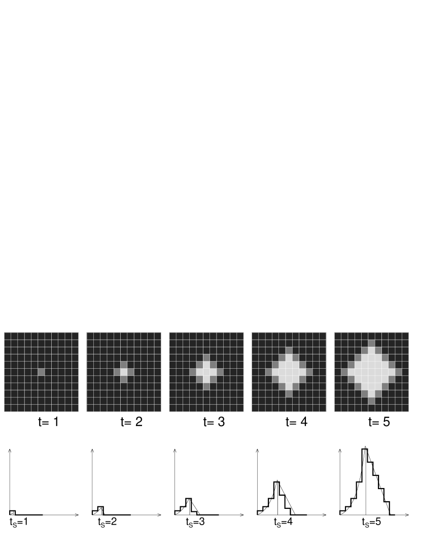
Figure 2.5: Spatial patterns of a propagating avalanche in subsequent time steps in a 2-D cellular automaton model with a next-neighbor redistribution rule (top) and time profiles of energy release rate (bottom), for saturation times of $t_{S}=1,2,...,5\Delta t$. The black cells represent cells with random fluctuations below the threshold, $z_{k}<z_{c}$, the grey cells contain possibly unstable cells with fluctuation $z_{k}\geq z_{c}$ that are subject to a first redistribution, while the white cells have already been affected by a redistribution rule before. Most avalanches die out after step t$\lower 1.54996pt\hbox{$\;\buildrel>\over{\scriptstyle\sim}\;$}2$.

In summary, this model predicts powerlaw distribution functions for the three SOC parameters $P$, $E$, and $T$, which match the simulated distributions with cellular automaton simulations, as well as the observed distributions of solar flare hard X-ray fluxes (Lu and Hamilton 1991). For a ratio of ${\tau_{G}/t_{S}}=1$, this model predicts $\alpha_{P}=2.0$, $\alpha_{T}=2.0$, and $\alpha_{E}=1.5$. This particular time ratio of ${\tau_{G}/t_{S}}=1$ implies that an avalanche typically saturates after one exponential growth time (see the spatio-temporal patterns for small avalanches in Fig. 2.5). Open questions are: Which physical process would explain this particular time scale ratio $\tau_{G}/t_{S}=1$ ? Why does the decay phase has a linear behavior? Is the exponential distribution of avalanche growth times consistent with observations, since powerlaw-like distributions are expected for SOC parameters? How can the observed intermittent fluctuations of time profiles and the fractal geometry be accomodated in a model with a monotonic growth function? Although this model seems not to reproduce all observed properties of SOC phenomena, it has a didactical value, since it represents the most basic model that links the nonlinear evolution of instabilities to the powerlaw distributions observed in SOC phenomena.

The exponential-growth model is most suitable for multiplicative avalanche processes, where the increase per time step during the rise phase is based on a multiplicative factor, such as it occurs in nuclear chain reactions, population growth, or urban growth. Alternatively, avalanche processes that continuously expand in space may show an energy increase that scales with the area or volume, which has a powerlaw relationship to the spatial or temporal scale, i.e., $A(t)\propto r(t)^{2}\propto t^{2}$ or $V(t)\propto r(t)^{3}\propto t^{3}$. Such a model with a powerlaw-growth function

$$W(t)=W_{0}\ \left[1+\left({t\over\tau_{G}}\right)^{p}\right]\ ,$$

rather than an exponential-growth function (Eq. 2.6) was computed in Aschwanden (2011a; Section 3.2), which predicts identical scaling laws between the SOC parameters ($P,E,T$), but the occurrence frequency distributions exhibit an exponential fall-off at the upper end. Otherwise it has similar caveats as the exponential-growth model (i.e., monotonic growth curve rather than intermittency, and Euclidean rather than fractal avalanche volume).

Another variant of the exponential-growth model is the logistic-growth model (Aschwanden 2011a; Section 3.3), which has a smoother transition from the initially exponential growth to the saturation phase, following the so-called logistic equation,

$${dE(t)\over dt}={\ E(t)\over\tau_{G}}\cdot\left[1-{E(t)\over E_{\infty}}\right]\ ,$$

where the dissipated energy is limited by the so-called carrying capacity limit $E_{\infty}$ used in ecological applications. The resulting occurrence frequency distributions are powerlaws for the energy $E$ and peak energy dissipation rate $P$, but exponential functions for the rise time $\tau$ and duration $T$ of an avalanche. Like the exponential-growth and the powerlaw-growth model, the temporal intermittency and the geometric fractality observed in real SOC phenomena are not reproduced by the smoothly-varying time evolution of the logistic-growth model.

2.2.2 The Fractal-Diffusive SOC Model (FD-SOC)

The microscopic structure of a SOC avalanche has been simulated with a discretized mathematical re-distribution rule, which leads to highly inhomogeneous, filamentary, and fragmented topologies during the evolution of an avalanche. Therefore, it appears to be adequate to develop an analytical SOC model that approximates the inhomogeneous topology of an avalanche with a fractal geometry. Bak and Chen (1989) wrote a paper entitled “The physics of fractals”, which is summarized in their abstract with a single sentence: Fractals in nature originate from self-organized critical dynamical processes.

A statistical fractal-diffusive avalanche model of a slowly-driven SOC system has been derived in Aschwanden (2012). This analytical model represents a universal (physics-free) description of the statistical time evolution and occurrence frequency distribution function of SOC processes. It is based on four fundamental assumptions: (1) A SOC avalanche grows spatially like a diffusive process; (2) The spatial volume of the instantaneous energy dissipation rate is fractal; (3) The time-averaged fractal dimension is the mean of the minimum dimension $D_{S,min}\approx 1$ (for a sparse SOC avalanche) and the maximum dimension $D_{S,max}=S$ (given by the Euclidean space); and (4) The occurrence frequency distribution of length scales is reciprocal to the size $L$ of spatial scales, i.e., $N(L)\propto L^{-S}$ in Euclidean space with dimension $S$. We will discuss these assumptions in more detail in the following.

The first assumption of a diffusive process is based on numerical simulations of cellular automaton models. A SOC avalanche propagates in a cellular automaton model by next-neighbor interactions in a critical state, where energy dissipation propagates only to the next neighbor cells (in a S-dimensional lattice grid) that are above a critical threshold. This mathematical rule that describes the entire dynamics and evolution of a SOC avalanche is very simple for a single time step, but leads to extremely complex spatial patterns after a finite number of time steps. For a visualization of a large number of such complex spatial patterns generated by a simple iterative mathematical redistribution rule see, for instance, the book “A New Kind of Science” by Wolfram (2002). The complexity of these spatial patterns can fortunately be characterized with a single number, the fractal dimension $D_{S}$. If one monitors the time evolution of a spatial pattern of a SOC avalanche in a cellular automaton model, one finds that the length scale $x(t)$ evolves with time approximately with a diffusive scaling (see radius $r(t)$ of snapshots of a 2-D cellular automaton evolution in Fig. (2.6) and its time evolution $r(t)\propto t^{1/2}$ in Fig. (2.8), bottom right panel),

$$x(t)\propto t^{1/2}\ ,$$

which leads to a statistical scaling law between the avalanche sizes $L=x(t=T)$ and time durations $T$ of SOC avalanches,

$$L\propto T^{1/2}\ .$$

Figure 2.6: Time evolution of a large avalanche event in a 2-D cellular automaton simulation with grid size $N=64^{2}$. The 12 panels show snapshots at particular burst times from $t=26$ to $t=690$ when the energy dissipation rate peaked. Active nodes where energy dissipation occurs at time $t$ are visualized with black and grey points, depending on the energy dissipation level. The starting point of the avalanche occurred at pixel $(x,y)=(41,4)$, which is marked with a cross. The time-integrated envelop of the avalanche is indicated with a solid contour, and the diffusive avalanche radius $r(t)=t^{1/2}$ is indicated with a dashed circle (Aschwanden 2012).

Figure 2.7: Determination of the fractal dimension $D_{2}=\log{A_{i}}/\log{x_{i}}$ for the instantaneous avalanche sizes of 6 time steps of the avalanche event shown in Fig. (2.6). Each row is a different time step and each column represents a different binning of macropixels ($\Delta x_{i}=1,2,4,8$). The fractal dimension is determined by a linear regression fit shown on the right-hand side. The mean fractal dimension of the 12 avalanche snapshots shown in Fig. (2.6) is $D_{2}=1.43\pm 0.17$ (Aschwanden 2012).

Figure 2.8: Time evolution of the same large avalanche event from a 2-D cellular automaton simulation with grid size $N=64^{2}$ as shown in Fig. (2.6). The time profiles include the instantaneous energy dissipation rate $f(t)=de/dt$ (top left), the time-integrated total energy $e(t)$ (bottom left), the instantaneous fractal dimension $D_{2}(t)$ (top right), and the radius of the avalanche area $r(t)$ (bottom right). The observed time profiles from the simulations are outlined in solid linestyle and the theoretically predicted average evolution in dashed linestyle. The statistically predicted values of the instantaneous energy dissipation rate $f(t)\propto t^{3/4}$ (dotted curve) and peak energy dissipation rate $p(t)\propto t^{1}$ (dashed curve) after a time interval $t$ are also shown (top left panel). The 12 time labels from 26 to 690 (top left frame) correspond to the snapshot times shown in Fig. (2.6) (Aschwanden 2012).

The second assumption of a fractal pattern of the instantaneous energy rate is also based on tests with cellular automaton simulations (see measured fractal dimensions $D_{2}$ of snapshots in Fig. (2.7) and the time evolution $D_{2}(t)$ in Fig. (2.8) top right panel). The fractal dimension is essentially a simplified parameter that describes the “micro-roughness”, “graininess”, or inhomogeneity of critical nodes in a lattice grid in the state of self-organized criticality. Of course, such a single number is a gross over-simplification of a complex system with a large number of degrees of freedom, but the numerical simulations confirm that avalanche patterns are fractal (Fig. 2.7). Thus we define the volume $V_{S}(t)$ of the instantaneous energy dissipation rate in terms of a fractal (Hausdorff) dimension $D_{S}$ that scales with the length scale $x$ as,

$$V_{S}(t)\propto x^{D_{S}}\ ,$$

which leads also to a statistical scaling law between avalanche volumes $V$ and spatial scales $L$ or durations $T$ of SOC avalanches (with Eq. 2.21)

$$V_{S}\propto L^{D_{S}}\propto T^{D_{S}/2}\ .$$

The third assumption of the mean fractal dimension has also been confirmed by numerical simulations of cellular automaton SOC processes in all three dimensions $S=1,2,3$ (Aschwanden 2012), but it can also be understood by the following plausibility argument. The sparsest SOC avalanche that propagates by next-neighbor interactions is the one that spreads only in one spatial dimension, and thus yields an estimate of the minimum fractal dimension of $D_{S,min}\approx 1$, while the largest SOC avalanche is almost space-filling and has a volume that scales with the Euclidean dimension, $D_{S,max}=S$. Combining these two extremal values, we can estimate a time-averaged fractal dimension $<D_{S}>$ from the arithmetic mean,

$$<D_{S}>\approx{D_{S,min}+D_{S,max}\over 2}={1+S\over 2}\ ,$$

which yields a mean fractal dimension of $<D_{3}>=(1+3)/2=2.0$ for the 3D case $(S=3)$.

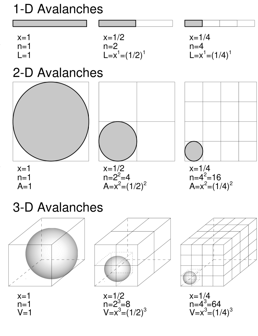
Figure 2.9: Schematic diagram of the Euclidean volume scaling of the diffusive avalanche boundaries, visualized as circles or spheres in the three Euclidean space dimensions $S=1,2,3$. The Euclidean length scale $x$ of subcubes decreases by a factor 2 in each step ($x_{i}=2^{-i},i=0,1,2$), while the number of subcubes increases by $n_{i}=(2^{i})^{S}$, defining a probability of $N(x_{i})\propto x_{i}^{-S}$ for each avalanche size with size $x_{i}$.

The fourth assumption on the size distribution is a probability argument. The system size $L_{sys}$ of a SOC system represents an upper limit of spatial scales $L$ for SOC avalanches, i.e., $L\leq L_{sys}$. For the 3D-case, the volumes $V$ of individual avalanches are also bound by the volume $V_{sys}$ of the system size, i.e., $V=L^{3}\leq V_{sys}=L_{sys}^{3}$. If the entire system is in a critical state, SOC avalanches can be produced everywhere in the system, and the probability $N(L)$ for a fixed avalanche size L with volume V is simply reciprocal to the size, (visualized in Fig. 2.9), i.e.,

$$N(V)\propto{V_{sys}\over V}\propto V^{-1}\ ,$$

which is equivalent to

$$N(L)\propto{L_{sys}^{3}\over L^{3}}\propto L^{-3}\ .$$

Based on these four model assumptions we can now quantify the time evolution of SOC parameters. For sake of simplicity we apply this fractal-diffusive SOC model to an astrophysical source that emits a photon flux $f(t)$ that is proportional to the instantaneous energy dissipation volume $V_{S}(t)$ of a SOC avalanche, where a mean energy quantum $<\Delta E>$ is emitted per volume cell element $\Delta V$. Thus, the emitted flux is (using the diffusive scaling $x(t)\propto t^{1/2}$),

$$f(t)={de(t)\over dt}\propto<\Delta E>V_{S}(t)=<\Delta E>x(t)^{D_{S}}=<\Delta E>t^{D_{S}/2}\ .$$

In the 2-D case with $D_{S}=D_{2}=(1+2)/2=3/2$ (Eq. 2.24) we expect a statistical scaling of $f(t)\propto t^{3/4}$ (see Fig. 2.8 top left). In the 3-D case with $D_{S}=D_{3}=(1+3)/2=2$, we expect than the proportionality $f(t)\propto t^{1}$. In Fig. (2.10) (second panel) we simulate such a flux time profile $f(t)$ by applying noise fluctuations in the time evolution of the fractal dimension $D_{2}(t)$ (Fig. 2.10, top).

The statistical peak value $p(t)$ of the energy dissipation rate after time $t$ can be estimated from the largest possible avalanches, which have an almost space-filling dimension $D_{S}\lower 1.72218pt\hbox{$\;\buildrel<\over{\scriptstyle\sim}\;$}S$,

$$p(t)={de(t)\over dt}\propto<\Delta E>V_{S,max}(t)=<\Delta E>x(t)^{S}=<\Delta E>t^{S/2}\ .$$

and thus would be expected to scale as $p(t)\propto t^{S/2}\propto t^{1.5}$ for the $S=3$ case. Thus the time profile of peak values envelopes the maximum fluctuations of the flux time profile $f(t)$ (Fig. 2.10, second panel).

The evolution of the total dissipated energy $e(t)$ after time $t$ is simply the time integral, for which we expect

$$e(t)=\int_{0}^{t}{de(\tau)\over d\tau}d\tau\propto\int_{0}^{t}\tau^{D_{S}/2}\propto t^{(1+D_{S}/2)}\ ,$$

which yields the function $e(t)\propto t^{7/4}$ for the 2-D case (Fig. 2.8, bottom left), and a function $e(t)\propto t^{2}$ for the 3-D case (Fig. 2.10, third panel). These time evolutions apply to every SOC model that has an emission $f(t)$ proportional to the fractal avalanche volume $V_{S}(t)$. For applications to observations in a particular wavelength range there may be an additional scaling law between the avalanche volume and emission (or intensity) of the underlying radiation mechanism.

The fourth assumption on the probability distribution of (avalanche) length scales,

$$N(L)\propto V_{S}^{-1}\propto L^{-S}\ .$$

is a simple probability argument, implying that the number or occurrence frequency of avalanches has an equal likelyhood throughout the system, so it assumes a homogeneous distribution of critical states across the entire system. This is an extremely important assumption, which automatically predicts a powerlaw distribution for length scales. Using the scaling laws that result from Eq. (2.21) and (2.27)-(2.29) for $L=x(t=T)$, $E=e(t=T)$, $F=f(t=T)$, and $P=p(t=T)$ for an avalanch duration time $T$,

$$\begin{array}[]{l}L\propto T^{1/2}\\ F\propto T^{D_{S}/2}\\ P\propto T^{S/2}\\ E\propto T^{1+D_{S}/2}\\ \end{array}\ ,$$

we can directly calculate the occurrence frequency distributions for all these SOC parameters, by substituting the variables from the correlative relationships given in Eq. (2.31), yielding

$$N(T)dT=N(L[T])\left|{dL\over dT}\right|dT\propto T^{-[(1+S)/2]}\ dT\ .$$

$$N(F)dF=N(T[F])\left|{dT\over dF}\right|dF\propto F^{-[1+(S-1)/D_{S}]}\ dF\ ,$$

$$N(P)dP=N(T[P])\left|{dT\over dP}\right|dP\propto P^{-[2-1/S]}\ dP\ ,$$

$$N(E)dE=N(T[E])\left|{dT\over dE}\right|dE\propto E^{-[1+(S-1)/(D_{S}+2)]}\ dE\ .$$

This derivation yields naturally powerlaw functions for all parameters $L$, $T$, $F$, $P$, and $E$, which are the hallmarks of SOC systems. In summary, if we denote the occurrence frequency distribution $N(x)$ of a parameter $x$ with a powerlaw distribution with power index $\alpha_{x}$,

$$N(x)dx\propto x^{-\alpha_{x}}\ dx\ ,$$

we have the following powerlaw coefficients $\alpha_{x}$ for the parameters $x=T,F,P$, and $E$,

$$\begin{array}[]{ll}\alpha_{T}&=(1+S)/2\\ \alpha_{F}&=1+(S-1)/D_{S}\\ \alpha_{P}&=2-1/S\\ \alpha_{E}&=1+(S-1)/(D_{S}+2)\\ \end{array}\ .$$

The powerlaw coefficients $\alpha_{x}$ and correlation are summarized in Table 2.2 separately for each Euclidean dimension $S=1,2,3$.

Table 2.2: Theoretically predicted occurrence frequency distribution powerlaw slopes $\alpha$ and power indices $\beta$ of parameter correlations predicted for SOC cellular automatons with Euclidean space dimensions $S=1,2,3$, for the fractal dimension $D_{S}$, length scale $L$, time duration $T$, instantaneous energy dissipation rate (or flux) $F$, peak energy dissipation rate (or peak flux) $P$, and total time-integrated energy $E$.

Theory	S=1	S=2	S=3
$D_{S}=(1+S)/2$	1	3/2	2
$\alpha_{L}=S$	1	2	3
$\alpha_{T}=(1+S)/2$	1	3/2	2
$\alpha_{F}=1+(S-1)/D_{S}$	1	5/3	2
$\alpha_{P}=2-1/S$	1	3/2	5/3
$\alpha_{E}=1+(S-1)/(D_{S}+2)$	1	9/7	3/2
$L\propto T^{1/2}$	$L\propto T^{1/2}$	$L\propto T^{1/2}$	$L\propto T^{1/2}$
$F\propto T^{D_{S}/2}$	$F\propto T^{1/2}$	$F\propto T^{3/4}$	$F\propto T^{1}$
$P\propto T^{S/2}$	$P\propto T^{1/2}$	$P\propto T^{1}$	$P\propto T^{3/2}$
$E\propto T^{1+D_{S}/2}$	$E\propto T^{3/2}$	$E\propto T^{7/4}$	$E\propto T^{2}$

These correlation coefficients and powerlaw indices of frequency distributions have been found to agree within $\approx 10\%$ with numerical simulations of cellular automatons for all three Euclidean dimensions ($S=1,2,3$) (Aschwanden 2011a). Some deviations, especially fall-offs at the upper end of powerlaw distributions, are likely to be caused by finite-size effects of the lattice grid.

2.2.3 Astrophysical Scaling Laws

SOC theory applied to astrophysical observations covers many different wavelength regimes, for instance gamma-rays, hard X-rays, soft X-rays, and extreme ultra-violet (EUV) in the case of solar flares. A comprehensive review of such studies is given in Section 7 of Aschwanden (2011a). However, since each wavelength range represents a different physical radiation mechanism, we have to combine now the physics of the observables with the (physics-free) SOC statistics.

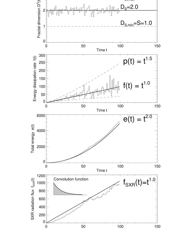
Figure 2.10: Simulation of the fractal-diffusive SOC model for an Euclidean dimension $S=3$, showing the time evolution of the fractal dimension $D_{S}(t)$ (top panel), the instantaneous energy dissipation rate $f(t)$ and peak energy dissipation rate $p(t)$ (second panel), the total time-integrated dissipated energy $e(t)$ (third panel), and the soft X-ray time profile $f_{sxr}(t)$ (bottom panel), which results from the convolution of the instantaneous energy dissipation rate $f(t)$ (second panel) with an exponential decay function with an e-folding time of $\tau_{decay}$ (shown in insert of bottom panel) (Aschwanden and Freeland 2012).

Let us consider soft and hard X-ray emission in solar or stellar flares. Soft X-ray emission during solar flares is generally believed to result from thermal free-free and free-bound radiation of plasma that is heated in the chromosphere by precipitation of non-thermal electrons and ions, and which subsequently flows up into coronal flare (or post-flare) loops, a process called “chromospheric evaporation process” (for a review see, e.g., Aschwanden 2004). Therefore, we can consider the flare-driven chromospheric heating rate as the instantaneous energy dissipation process of a SOC avalanche, as shown in the simulated function $f(t)$ in Fig. 2.10 (second panel). The heated plasma, while it fills the coronal flare loops, loses energy by thermal conduction and by radiation of soft X-ray and EUV photons, which generally can be characterized by an exponential decay function after an impulsive heating spike. In Fig. 2.10 (bottom) we mimic such a soft X-ray radiation light curve by convolving the instantaneous energy dissipation rate $f(t)$ (Fig. 2.10, second panel) with an exponentially decaying radiation function (with an e-folding time constant of $\tau_{decay})$,

$$f_{sxr}(t)=\int_{-\infty}^{t}f(t)\exp{\left[-{(t-t^{\prime})\over\tau_{decay}}\right]}dt^{\prime}\ ,$$

which shows also a time dependence that follows approximately

$$f_{sxr}(t)\propto f(t)\propto t^{1.0}\ ,$$

because the convolution with an exponential function with a constant e-folding time constant acts like a constant multiplier. In the limit of infinitely long decay times $(\tau_{decay}\mapsto\infty)$, our convolution function (Eq. 2.38) turns into a time integral of the heating function $f(t)$, which is also known as Neupert effect (Dennis and Zarro 1993; Dennis et al. 2003).

The heating function is identified with the non-thermal hard X-ray emission, which indeed exhibits a highly fluctuating and intermittent time profile for energies of $\lower 1.72218pt\hbox{$\;\buildrel>\over{\scriptstyle\sim}\;$}25$ keV, where non-thermal emission dominates,

$$f_{hxr}(t)\propto p(t)\propto t^{1.5}\ ,$$

Thus the occurrence frequency distributions of fluxes are expected to be different for soft X-rays and hard X-rays, the hard X-ray flux $f_{hxr}(t)$ follows the statistics of the highly fluctuating peak energy dissipation rate $p(t)$, while the soft X-ray flux $f_{sxr}(t)$ is expected to follow the statistics of the smoothly-varying (convolved) time profile $f(t)$. The total duration $T$ of energy release of an avalanche (or flare here) corresponds essentially to the rise time $t_{rise}$ of the soft X-ray flux, or to the total flare duration for hard X-rays, because the decay phase of a soft X-ray flare light curve is dominated by conductive and radiative loss, rather than by continued heating input. Thus based on the generic relationships summarized in Table 2.2 we expect for the 3-D case ($S=3$),

$$N(T)\propto T^{-\alpha_{T}}=T^{-2}\ ,$$

$$N(f_{sxr})\propto F^{-\alpha_{F}}=F^{-[1+(S-1)/D_{S}]}=F^{-2}\ ,$$

$$N(f_{hxr})\propto P^{-\alpha_{P}}=P^{-[2-1/S]}=P^{-5/3}\ .$$

Applications to observations did show satisfactory agreement with these theoretical values, i.e. powerlaw slopes of $\alpha_{F}=2.0$ for soft X-rays and $\alpha_{P}=1.67$ for hard X-rays (Aschwanden 2011a; 2011b; Aschwanden and Freeland 2012), except for the occurrence frequency distributions of flare durations $T$ during solar cycle maxima, when the flare pile-up bias appears to have a steepening side-effect (Aschwanden 2012).

2.2.4 Earthquake Scaling Laws

While the foregoing discussion is relevant to astrophysical SOC phenomena (solar and stellar flares), similar physical scaling relationships between the observables and SOC cellular automaton quantities $z_{i,j,k}$ can be developed in other fields. For earthquakes in geophysics for instance, measured quantities include the length $L_{S}$ and width $L_{w}$ of a rupture area, so the rupture area has the scaling $A\propto L_{S}L_{w}$. For large ruptures, however, when the surface rupture length is much larger than the rupture width, i.e., $L_{s}\gg L_{w}$, the width $L_{w}$ was found to be approximately constant, so that large ruptures saturate the faults surface and scale with a fractal dimension of $D=1$, whereas a smaller rupture propagates across both dimension $(D=2)$ of the fault face (Yoder et al. 2012). The modeling of size distributions of earthquake magnitudes can then be conducted with a similar methodology as outlined with our fractal-diffusive model (Section 2.2.2), requiring: (i) The definition of the Euclidean space dimension for earthquakes, which could be $S=2$ if they are treated as surface phenomena without significant depth variability, or by $S=3$ otherwise; (ii) The measurement of the fractal dimension $D$, which can exhibit multi-fractal scaling from $D=1$ for large earthquakes to $D=2$ for small earthquakes; and (iii) assigning the observable $m$, which is the magnitude of the earthquake, to the corresponding physical quantity, i.e., the peak energy dissipation rate $P$, the smoothed energy dissipation rate $F$, or total time-integrated energy $E$. Furthermore, earthquake size distributions are often reported in terms of a cumulative distribution function $N(>m)$, which has a powerlaw index $\beta\approx\alpha-1$ that is flatter by one than the differential distribution function $N(m)dm$.

2.3 Alternative Models Related to SOC

Here we discuss a number of alternative dynamical models that are related to SOC models or have similar scaling laws, and discuss what they have in common with SOC or where they differ. A metrics between processes and observables is synthesized in Fig. 2.15.

2.3.1 Self-Organization Without Criticality (SO)

Self-organization (SO) is often referred to geometric patterns that originate by mutual interaction of their elements, without coordination from outside the system. For instance, convection arranges itself into a regular pattern of almost equal-sized convection cells, a structuring process also known as Bénard cells. Other examples are the regular wavy pattern of sand dunes in the desert, wavy patterns of Cirrus clouds in the Earth atmosphere, Jupiter’s atmosphere with white bands of ammonia ice clouds, the spiral-like patterns of the Belousov-Zhabotinsky reaction-diffusion system, or geometric patterns in biology, such as the skin of zebras, giraffes, tigers, tropical fishes, or formation flight of birds. From these examples we see that self-organization mostly refers to the self-assembly of geometric patterns, which are more or less stable over long time intervals, although they arise from the physics of non-equilibrium processes, which can involve diffusion, turbulence, convection, or magneto-convection, which are governed by long-range interactions (via pressure and forces).

What is the difference to self-organized criticality (SOC)? Are sandpile avalanches a self-organizing (SO) pattern? In the standard scenario of the sandpile SOC model, individual avalanches are a local phenomenon that are randomly triggered in space and time, but occur independently, at least in the slowly-driven case. Thus, one avalanche has no mutual interaction with another avalanche and the outcome of the final size is independent of another, in contrast to self-organization without criticality, where the interaction between system-wide structures is coupled. In other words, sandpile avalanches are governed by localized disturbances via next-neighbor interactions, while self-organizing patterns may be formed by both next-neighbor and long-range interactions. Another difference is that SO creates spatial patterns, while SOC generates dynamical events (i.e., avalanches). Also the statistical distributions of the two processes are different. A self-organizing pattern is likely to produce a preferred size scale (e.g., the solar granulation or the width of zebra stripes), while self-organized criticality produces a scale-free powerlaw distribution of avalanche sizes. The difference between SO and SOC could may be best illustrated with a sandpile analogy. The same sandpile can be subject to self-organization (SO), for instance when a steady wind blows over the surface and produces wavy ripples with a regular spacing pattern, as well as be subject to self-organized criticality (SOC), when intermittent avalanches occur due to random-like disturbances by infalling sand grains. The former geometric pattern may appear as a spatial-periodic pattern, while the latter may exhibit a fractal geometry.

2.3.2 Forced Self-Organized Criticality (FSOC)

In Bak’s original SOC model, which is most genuinely reproduced by sandpile avalanches and cellular automaton simulations, criticality is continuously restored by next-neighbor interactions. If the local slope becomes too step, an avalanche will erode it back to the critical value. If the erosion by an avalanche flattened the slope too much, it will be gradually restored by random input of dropped sand grains in the slowly-driven limit. When the observations were extended to magnetospheric substorms in the night-side geotail, powerlaw-like size distributions were found, suggesting a self-organized criticality process, but at the same time correlations with magnetic reconnection events at the dayside of the magnetosphere were identified, driven by solar wind fluctuations, suggesting some large-scale transport processes and long-range coupling between the day-side and night-side of the magnetosphere. Thus, these long-range interactions that trigger local instabilities in the current sheet in the Earth’s magnetotail were interpreted as external forcing or loading, and a combined forced and/or self-organized criticality (FSOC) process was suggested (Chang 1992, 1998a,b, 1999a,b). A forced SOC process may apply to a variety of SOC phenomena in the magnetosphere, such as magnetotail current disruptions (Lui et al. 2000), substorm current disruptions (Consolini and Lui 1999), bursty bulk flow events (Angelopoulos et al. (1996, 1999), magnetotail magnetic field fluctuations (Hoshino et al. 1994), auroral UV blobs (Lui et al. 2000; Uritsky et al. 2002), auroral optical blobs (Kozelov et al. 2004), auroral electron (AE) jets (Takalo et al. 1993; Consolini 1997), or outer radiation belt electron events (Crosby et al. 2005).

What distinguishes the FSOC model from the standard (BTW-type) SOC model is mostly the long-range coupling, which is absent in sandpiles and cellular automaton models. The driving force in the FSOC model is a long-distance action (loading process), while it is a random local disturbance in the BTW model. Otherwise, the FSOC model entails also powerlaw distributions for the avalanche events, fractality, intermittency, statistical independence of events (indicated by random waiting time distributions), and a critical threshold (for the onset of local plasma instabilities and/or magnetic reconnection processes).

Figure 2.11: Numerical simulation of 1D Brownian random walk (left side) and size increase of a 2D cellular automaton avalanche (right side) as a function of time $t$. Both processes follow the trend $x(t)\propto t^{1/2}$ expected for classical diffusion.

2.3.3 Brownian Motion and Classical Diffusion

Brownian motion is a concept from classical physics that describes the random motion of atoms or molecules in a gas (named after the Scottish botanist Robert Brown), which can be best observed when a neutral gas of a different color is released in the atmosphere. What we observe then is an isotropic diffusion process (in the absence of forces or flows) that monotonically increases with the square-root of time,

$$<x(t)>\propto t^{1/2}\ .$$

This statistical trend was derived in classical thermodynamics, assuming a Gaussian distribution of velocities for the gas molecules, so that the kinetic energy of particles follow a Boltzmann distribution in thermodynamic equilibrium. The classical diffusion process can also be described by a differential equation for a distribution function $f(x,t)$ of particles,

$${\partial f(x,t)\over\partial t}=\kappa{\partial^{2}f(x,t)\over\partial x^{2}}\ ,$$

which can describe heat transport, diffusion of gases, or magnetic diffusivity on solar and stellar surfaces (i.e., manifested as meridional flows during a solar/stellar activity cycle).

An example of such a diffusive random walk is simulated in Fig. 2.11 (left panel) for the 1-D variable $x(t)$. We have to be aware that a diffusive random walk $x(t)$ of a single particle can show large deviations from the expected trend $\propto t^{1/2}$, which is only an expectation value for the statistical mean of many random walks $<x(t)>=\sum_{i}x_{i}(t)$. In Fig. 11 (right panel) we show also the time evolution of the mean radius $<r(t)>$ of a simulated cellular automaton avalanche (taken from Fig. 2.8, bottom right), which shows the same trend of a time-dependence of $r(t)\propto t^{1/2}$. Apparently, the enveloping volume of unstable cells in a SOC avalanche, defined by the a mathematical re-distribution rule applied to a coarse-grained lattice with a rough surface of stable, meta-stable, and unstable nodes produces a similar time evolution as a random walk (as visualized in Fig. 2.6), leading us to the fractal-diffusive SOC model described in Section 2.2.2. This behavior of a diffusive transport process is therefore common to both the Brownian motion (or classical diffusion) and to a cellular automaton SOC process, but it operates for a SOC process only during a finite time interval, as long as avalanche propagation is enabled by finding unstable next neighbors, while a classical diffusion process goes on forever without stopping. Therefore, we cannot define an event and occurrence frequency distributions. However, we can measure the fractal dimension of a random walk spatial pattern, which has a Hausdorff dimension of $D_{2}=2$ in 2-D Euclidean space, or the power spectrum, i.e., $P(\nu)\propto\nu^{-2}$, also called Brownian noise.

Figure 2.12: Noise power spectra (left panels) and corresponding time series (right panels) for power spectral indices $p=0$ (top row: white noise spectrum), $p=1$ (second row: pink noise spectrum), $p=2$ (third row: red noise spectrum), and $p=3$ (bottom row: black noise spectrum). The white noise spectrum is multiplied with $\nu^{-p}$ in the other cases. The time series are reconstructed with the inverse Fast Fourier Transform (Aschwanden 2011a).

Table 2.3: Nomenclature of noise spectra.

Power spectrum	Power index	Spectrum nomenclature
$P(\nu)\propto\nu^{0}$	$p=0$	white noise
$P(\nu)\propto\nu^{-1}$	$p=1$	pink noise, flicker noise, $1/f$ noise
$P(\nu)\propto\nu^{-2}$	$p=2$	red noise, Brown(ian) noise
$P(\nu)\propto\nu^{-3}$	$p=3$	black noise

Generalizations that include power spectra $P(\nu)\propto\nu^{-\beta}$ with arbitrary powerlaw indices $\beta$ have been dubbed fractional Brownian motion (fBM), for instance white noise ($\beta=0$, where subsequent steps are uncorrelated), 1/f-noise, flicker noise, or pink noise ($\beta=1$), Brownian noise or red noise ($\beta=2$), or black noise ($\beta=3$, where subsequent time steps have some strong correlations, producing slowly-varying time profiles). The latter fluctuation spectrum has been found to describe the stock market well. Examples for these different types of fractional Brownian motion are given in Fig. 2.12, while the nomenclature of noise spectra is summarized in Table 2.3.

2.3.4 Hyper-Diffusion and Lévy Flight

The cellular automaton mechanism, the prototype of SOC dynamics, involves a mathematical re-distribution rule amongst the next neighbor cells (Eq. 2.1). This discretized numerical re-distribution rule has been transformed in the continuum limit to an analytical function $A(x,t)$, which can be expressed as fourth-order hyper-diffusion equation (Liu et al. 2002; Charbonneau et al. 2001),

$${\partial A\over\partial t}=-\kappa{\partial^{4}A\over\partial x^{4}}=-{\partial^{2}A\over\partial x^{2}}\kappa(A^{2}_{xx}){\partial^{2}A\over\partial x^{2}}\ ,$$

where $A$ represents the placeholder of the physical quantity corresponding to the symbol $z_{i,j,k}$ in Eq. 2.1, $x$ is the S-dimensional space coordinate ($x_{i,j,k}$ for $S=3$), with second-order centered differencing in space, forward differencing in time, and $\kappa=1/2S$ the hyper-diffusion coefficient for Euclidean dimension $S$. However, in contrast to classical physics, the hyper-diffusion coefficient $\kappa$ is subject to a threshold value in the SOC model,

$$\kappa=\left\{\begin{array}[]{ll}\kappa_{a}&{\rm if}\quad\Delta A^{2}>A_{crit}^{2}\\ 0&{\rm otherwise}\\ \end{array}\right.\ .$$

So, on a basic level, the evolution of a cellular automaton avalanche translates into a hyper-diffusion process, as demonstrated in Liu et al. (2002). How can it be described by classical diffusion as we discussed in the foregoing Section and in the fractal-diffusive SOC model in Section 2.2.2? The major difference of the two apparently contradicting descriptions lies in the fractality: The fourth-order hyper-diffusion system (subjected to a threshold instability in the diffusion coefficient $\kappa$) is applied to a Euclidean space with dimension $S$, while the fractal-diffusive SOC model has a second-order (classical) diffusion coefficient in a fractal volume $V_{S}\propto x^{D_{S}}$ with a fractal dimension $D_{S}\approx(1+S)/2$. The two diffusion descriptions apparently produce an equivalent statistics of avalanche volumes $V_{S}$, as demonstrated by the numerical simulations of powerlaw distribution functions $N(V_{S})$ by both models (Liu et al. 2002).

Other modifications of random walk or diffusion processes have been defined in terms of the probability distribution function of step sizes. Classical diffusion has a normal (Gaussian) distribution of step sizes, which was coined Rayleigh flight by Benoit Mandelbrot, while Lévy flight was used for a heavy-tailed probability distribution function (after the French mathematician Paul Pierre Lévy). Related are also the heavy-tailed Pareto probability distribution functions. Thus, Lévy flight processes include occasional large-step fluctuations on top of classical diffusion, which is found in earthquake data, financial mathematics, cryptography, signal analysis, astrophysics, biophysics, and solid state physics. A number of SOC phenomena have been analyzed in terms of Lévy flight processes, such as rice piles (Boguna and Corral 1997), random walks in fractal environments (Hopcraft et al. 1999; Isliker and Vlahos 2003), solar flare waiting time distributions (Lepreti et al. 2001), or extreme fluctuations in the solar wind (Moloney and Davidsen 2010, 2011).

2.3.5 Nonextensive Tsallis Entropy

Related to Lévy flight is also the nonextensive Tsallis entropy, which originates from the standard extensive Boltzmann-Gibbs-Shannon (BGS) statistics, where the entropy $S$ is defined as,

$$S=-k_{B}\sum p_{i}\ln p_{i}\ ,$$

with $k_{B}$ the Boltzmann constant and $p_{i}$ the probabilities associated with the microscopic configurations. The standard BGS statistics is called extensive when the correlations within the system are essentially local (i.e., via next-neighbor interactions), while it is called nonextensive in the case when they are non-local or have long-range coupling, similar to the local correlations in classical diffusion and non-local steps in the Lévy flights. As an example, the dynamic complexity of magnetospheric substorms and solar flares has been described with nonextensive Tsallis entropy in Balasis et al. (2011). Although nonlocal interactions are not part of the classical BTW automaton model, the extensive Tsallis entropy produces statistical distributions with similar fractality and intermittency. The nonextensive Tsallis entropy has a variable parameter $q$,

$$S_{q}=k{1\over q-1}\left(1-\sum_{i=1}^{W}p_{i}^{q}\right)\ ,$$

where $q$ is a measure of the nonextensivity of the system. A value of $q=1$ corresponds to the standard extensive BGS statistic, while a larger value $q>1$ quantifies the non-extensivity or importance of long-range coupling. A value of $q=1.84$ was found to fit data of magnetospheric substorms and solar flare soft X-rays (Balasis et al. 2011).

2.3.6 Turbulence

Turbulence is probably the most debated contender of SOC processes, because of the many common observational signatures, such as the (scale-free) powerlaw distributions of spatial and temporal scales, the power spectra of time profiles, random waiting time distributions, spatial fractality, and temporal intermittency.

Let us first define turbulence. Turbulence was first defined in fluid dynamics in terms of the Navier-Stokes equation. A fluid is laminar at low Reynolds numbers (say at Reynolds numbers of $R\lower 1.72218pt\hbox{$\;\buildrel<\over{\scriptstyle\sim}\;$}5000$, defined by the dimensionless ratio of inertial to viscous forces, i.e., $R=vL/\nu_{visc}$ with $v$ the mean velocity of an object relative to the fluid, $L$ the characteristic linear dimension of the fluid, and $\nu_{vis}$ the kinematic viscosity), while it becomes turbulent at high Reynolds numbers.

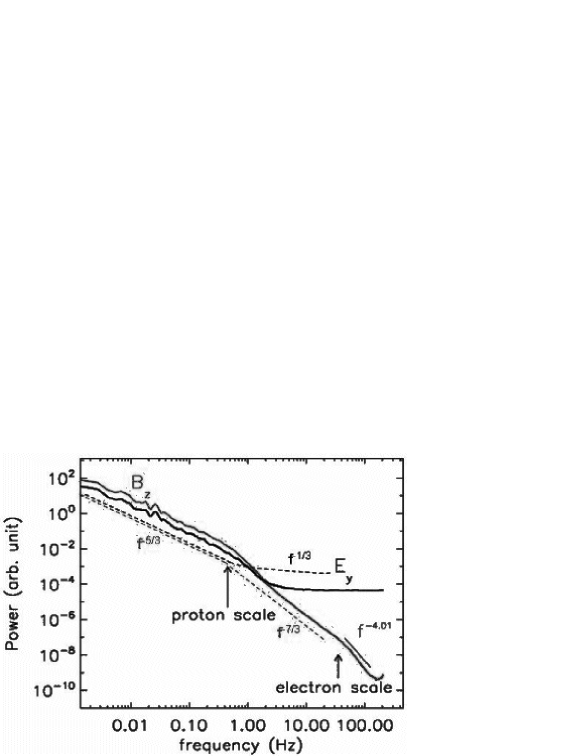
Figure 2.13: A spectrum of the solar wind is shown, based on CLUSTER observations from large to small scales, with the proton and electron gyroradius scale indicated. The solar wind spectrum is interpreted in terms of a turbulent MHD cascade, with the theoretically predicted slopes of $f^{-5/3}$ and $f^{-7/3}$ from gyro-kinetic theory. The plot proves that the energy continues cascading below the proton scale down to the electron scale, where it is converted to heat (via electron Landau damping resonance) causing the steepening of the $B_{z}$ spectrum to $f^{-4}$ (Howes et al. 2008; Sahraoui et al. 2009; credit: ESA, CLUSTER).

SOC phenomena and turbulence have been studied in astrophysical plasmas (such as in the solar corona, in the solar wind, or in stellar coronae), where the magneto-hydrodynamic (MHD) behavior of the plasma is expressed with the continuity equation, the momentum equation and induction equation,

$$\rho{D{\bf v}\over Dt}=-\nabla p-\rho{\bf g}+({\bf j}\times{\bf B})+{\nu}_{visc}\rho\left[\nabla^{2}{\bf v}+{1\over 3}\nabla(\nabla\cdot{\bf v})\right]\ ,$$

$${\partial{\bf B}\over\partial t}=\nabla\times({\bf v}\times{\bf B})+{\eta}_{m}\nabla^{2}{\bf B}\ ,$$

with $\rho$ being the plasma density, $p$ the pressure, ${\bf B}$ the magnetic field, ${\bf j}$ the electric current density, $\nu_{visc}$ the kinematic viscosity or shear viscosity, $\eta_{m}=c^{2}/4\pi\sigma$ the magnetic diffusivity, and $\sigma$ the electric conductivity. In the solar corona and in the solar wind, the magnetic Reynolds number is sufficiently high ($R_{m}=vL/\eta_{m}\approx 10^{8}-10^{12}$) to develop turbulence. Turbulence in the coronal plasma or in the solar wind is created by initial large-scale disturbances (for instance by the convective random motion in sub-photospheric layers or by the shock-like expansion of flares and coronal mass ejections). The large-scale disturbances pump energy into the coronal magnetic field or heliospheric solar wind at large scales, which cascade in the case of turbulent flow to smaller scales, where the energy can be more efficiently dissipated by friction, which is quantified by the kinematic or (Braginskii) shear viscosity coefficient $\nu_{visc}$. Ultimately, the energy of an MHD turbulent cascade is dissipated in the solar wind at the spatial scale of (gyrating) thermal protons ($\approx 50$ km), and at the scale of thermal electrons ($\approx 0.5$ km). The resulting power spectrum of the solar wind shows a power spectrum of $P(\nu)\propto\nu^{-5/3}$ at frequencies below the proton scale, $P(\nu)\propto\nu^{-7/3}$ between the proton and electron scale, and $P(\nu)\propto\nu^{-4}$ beyond the electron scale (Fig. 2.13). For literature references on MHD turbulence in the solar corona and in the solar wind see, e.g., Aschwanden (2011a, Section 10.4 therein).

What is the relationship between turbulence and SOC processes? The transition from laminar flow to turbulent flow at a critical Reynolds number $R_{crit}$ represents a similar thresholded instability criterion as the critical value $z_{crit}$ in SOC systems, above which a turbulent avalanche could occur with subsequent cascading from vortices at large scales and little energy dissipation towards smaller scales with stronger energy dissipation. Turbulent energy dissipation probably reduces the mean velocity of the fluid particles that are faster than the background flow and laminar flow could be restored with lower particle velocities and a lower Reynolds number. To make this process self-organizing, we need also a driver mechanism that brings the fluid speed back up to the critical Reynolds number. In the solar wind, for instance, there is systematic acceleration with heliocentric distance, which could drive the system from laminar back to turbulent flows, and thus it could be self-organizing. Fluctuations of the solar wind speed could therefore be considered as SOC avalanches. This could explain the scale-free powerlaw distributions of spatial, temporal, and energy scales measured in solar wind fluctuations, its fractality and intermittency. If the critical threshold is exceeded only in localized regions, rather than in the entire system in a fully turbulent state, energy dissipation would also occur in locally unstable regions, similar to SOC avalanches, and thus the two processes may exhibit the same statistical distributions. Consequently, turbulence could qualify as a SOC process if it is driven near the laminar-turbulent critical Reynolds number in a self-organizing way. However, fully developed turbulence, where the entire system is governed by a high (super-critical) Reynolds number, would correspond to a fast-driven SOC system in a catastrophic phase with permanent avalanching, without restoring the critical state as in a slowly-driven SOC system.

2.3.7 Percolation

Percolation is a dynamic process that depends on the connectedness and propagation probability of next-neighbor elements, and has a lot in common with diffusion, fractal structures, and SOC avalanches. A classical paradigm of a percolation process is coffee percolation, which contains a solvent (water), a permeable substance (coffee grounds), and soluble constituents (aromatic chemicals). The bimodal behavior of a percolation process can be best expressed with the observation whether a liquid that is poured on top of some porous material, will be able to make its way from hole to hole and reach the bottom. The answer will very much depend on the inhomogeneity characteristics of the porous material. In the subcritical state, a percolating cluster will exponentially die out, while it will propagate all the way to the bottom in a supercritical state. The process can be described by branching theory, where the connections between two next neighbors can be open and let the liquid pass with probability $p$, or they can be closed and the probability to pass is $(1-p)$. Completion of a pass from the top to the bottom can be expressed as the combined statistical probability along the entire pass. The critical value $p_{crit}$ that decides between the two outcomes is $p_{crit}=1/2$ for a 2-D process. So, this process has an extreme sensitivity to the system probability $p$, depending whether it is below or above the critical value. In SOC systems, the outcome of an avalanche is independent of the initial conditions of the triggering disturbance. Also, the material in a percolation process has a constant value of $p$ and does not self-adjust to a critical value, and thus it does not behave like a SOC system. However, what a percolation process has in common with a SOC system is the fractality and intermittency of propagating features. Other applications of percolation theory are used in physics, material science, complex networks, epidemiology, and geography.

2.3.8 Phase Transitions

In classical thermodynamics, a phase transition describes the transformation of one phase to another state of matter (solid, liquid, gas, plasma). For instance, transitions between solid and liquid states are called “freezing” and “melting”, between liquid and gas are “vaporization” and “condensation”, between gas and plasma are “ionization” and “deionization”. Phase transitions from one state to another can be induced by changing the temperature and/or pressure.

Since there are critical values of temperature and pressure that demarcate the transitions, such as the freezing temperature at $0^{0}$ C or the boiling point of $100^{0}$ C, we may compare these critical limits with the critical threshold $z_{crit}$ in SOC systems. Could this critical value be restored in a self-organizing way? To some extent, the daily weather changes can be self-organizing. Let us assume some intermediate latitude on our planet where the temperature is around the freezing point at some seasonal period, say Colorado or Switzerland around November. The temperature may drop below the freezing point during night, triggering snowfall, and may raise slightly above freezing point during sunny days, triggering melting of snow. In this case, the day-night cycle or the Earth’s rotation causes the temperature to oscillate around the freezing point, and therefore is in a self-organizing state. Additional variation of cloud cover may introduce fluctuations on even shorter time scales. However, this bimodal behavior of the temperature is not a robust operation mode of self-organized criticality, because seasonal changes will bring the average daily temperature systematically out of the critical range around the freezing point. So, such temporary fluctuations around a critical point seem to be consistent with a SOC system only on a temporary basis or in intermittent (seasonal) time intervals. In fact, a number of metereological phenomena have been found to exhibit powerlaw distributions and where associated with SOC behavior, such as Nile river fluctuations (Hurst 1951), rainfall (Andrade et al. 1998), cloud formation (Nagel and Raschke 1992), climate fluctuations (Grieger 1992), aerosols in the atmosphere (Kopnin et al. 2004), or forest fires (Kasischke and French 1995, Malamud et al. 1998). Phase transitions may be involved in some of these processes (rainfall, cloud formation, forest fires).

Phase transitions are also involved in some laboratory experiments in material or solid-state physics, quantum mechanics, and plasma physics, that have been associated with SOC behavior, if we extend the term phase transition also to morphological changes between highly-ordered and/or chaotic-structured patterns. Such phase transitions with SOC behavior have been found in transitions between the ferromagnetic and paramagnetic phases, in specimens of ferromagnetic materials settling into one of a large number of metastable states that are not necessarily the energetically lowest ones (Che and Suhl 1990), in avalanche-like topological rearrangements of cellular domain patterns in magnetic garnet films (Babcock and Westervelt 1990), in the noise in the magnetic output of a ferromagnet when the magnetizing force applied to it is charged (Cote and Meisel 1991), called the Barkhausen effect, in superconducting vortex avalanches in the Bean state (Field et al. 1995), in tokamak plasma confinement near marginal stability driven by turbulence with a subcritical resistive pressure gradient (Carreras et al. 1996), or in the electrostatic floating potential fluctuations of a DC glow charge plasma (Nurujjaman and Sekar-Iyenbgar 2007).

In summary, many SOC phenomena are observed during phase transitions, producing avalanche-like rearrangements of geometric patterns, but a phase-transition is not necessarily self-organizing in the sense that the critical control parameter stays automatically tuned to the critical point. A sandpile maintains its critical slope automatically in a slowly-driven operation mode. If a thermostat would be available, temperature-controlled phase transitions could be in a self-organized operation mode, which indeed can be arranged in many situations. So we conclude that phase transitions with some kind of “thermostat” tuned to the critical point represent indeed SOC systems.

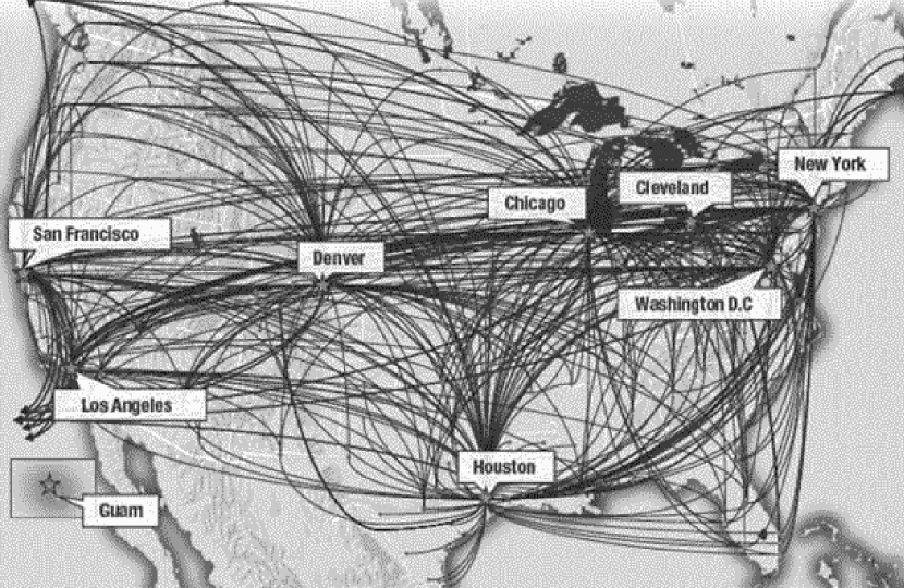
Figure 2.14: Network of American airline UNITED with 8 US-based hubs and connections to 378 destinations in 59 countries (Credit: United).

2.3.9 Network Systems

The prototype of a SOC cellular automaton model is a regular lattice grid, where re-distributions occur with next neighbors cells. In contrast, networks are irregular nets of nodes that are inter-connected in manifold patterns, containing not necessarily only next-neighbor connections, but also arbitrary non-local, long-range connections. Popular examples of networks are subway maps, city maps, road maps, airplane route maps, electric grid maps, social networks, company organizational charts, financial networks, etc, all being created by human beings in some way or another. One big difference to SOC systems is therefore immediately clear, the addition of long-range connections. Furthermore, while the statistical probabilities for next-neighbor interactions are identical for each lattice point in a SOC cellular automaton model, networks can have extremely different connection probabilities at each node point. Nodes that have most of the connections are also called hubs. For instance, the American airline United has 378 destinations, but server most of them from 10 hubs (Denver, Washington DC, San Francisco, Los Angeles, Chicago, Houston, Cleveland, Newark, Narita, Guam) (Fig. 14). Since the connection probability varies greatly from node to node, we do expect different clustering patterns in networks and in SOC lattice systems.

Nevertheless, SOC behavior has been studied in network systems like city growth and urban growth (Zipf 1949; Zanette 2007), cotton prizes (Mandelbrot 1963), financial stock market (Scheinkman and Woodford 1994; Sornette et al. 1996; Feigenbaum 2003; Bartolozzi et al. 2005), traffic jam (Bak 1996; Nagel and Paczuski 1995), war casualties (Richardson 1941, Levy 1983), social networks (Newman et al. 2002), internet traffic (Willinger et al. 2002), and language (Zipf 1949). SOC phenomena with powerlaw-like frequency distributions have been observed for phenomena that occur in these networks, measured by some quantity that expresses fluctuations above some threshold or noise level. Spatial patterns of network phenomena have been found to be fractal, and time profiles of these fluctuations were found to be intermittent, all hallmarks of SOC systems. So, are those network phenomena self-organizing? What is the critical threshold and what drives the system back to the critical threshold? The driving force of cotton prices, lottery wins, and stockmarket fluctuations is simply the human desire to gain money and to make profit. The driving mechanism for traffic jams is certainly the daily need for commuting and transportation in a finite road network. The unpredictable number of casualties in crimes and wars is a bit more controversial, but nobody would disagree that the human desire for power and control plays a role. The driving mechanism for social networks is most likely linked to curiosity and desire for information. Since all these human traits are quite genuine and persistent, a self-organizing behavior is warranted, where the system is continuously driven towards a critical state, with occasional larger fluctuations (Wall Street crash, Second World War, or other “social catastrophes”), on top of the daily fluctuations on smaller scales. In summary, most network-related phenomena can exhibit SOC behavior, apparently with similar powerlaw-like statistics in grids with non-uniform connectivities and non-local long-range connections (in network systems) as in regular lattice grids with next-neighbor interactions only (in classical SOC systems).

2.3.10 Chaotic Systems

Chaotic systems are nonlinear dissipative dynamical processes that are in principle deterministic, but exhibit “chaotic” behavior in the sense of irregular and fractal geometry, and intermittent time evolution. Some chaotic systems can be described as simple as with two (such as the Lotka-Volterra equation) or three coupled differential equations (e.g., the Lorenz equations). Classical examples include forced pendulum, fluids near the onset of turbulence, lasers, nonlinear optical devices, Josephson junctions, chemical reactions, the three-body system in celestial mechanics, ecological population dynamics, or the heartbeat of biological organisms (e.g., Schuster 1988). If two dynamical variables (say $x(t)$ and $y(t)$) are plotted in phase space ($y$ versus $x$), chaotic systems often exhibit a cyclic behavior, with a limit cycle that is also called strange attractor. If a dynamical system is driven from small disturbances around an equilibrium solution, where it exhibits a quasi-linear behavior, bifurcations of system variables $x(t)$ can occur at critical values with transitions to chaotic and intermittent behavior (also called route to chaos). Such bifurcations ressemble the phase transitions we discussed earlier (Section 2.3.8), which we generalized to transitions from highly-ordered to chaotic-structured patterns. The complexity of nonlinear chaotic systems is often characterized with the dimension of strange attractors (e.g., Grassberger 1985; Guckenheimer 1985), which approximately corresponds to the number of coupled differential equations that is needed to describe the system dynamics.

If we compare the dynamics of chaotic systems with SOC processes, a major difference is the deterministic evolution of chaotic systems, while SOC avalanches are statistically independent of each other, even when they occur subsequently within a small (waiting) time interval. A chaotic system evolves with a system-wide dynamical behavior that is influenced by the entire system, as the coupled differential equations express it, which includes next neighbors as well as non-local, long-range coupling, while an avalanche in a SOC system occurs only as a result of next-neighbor interactions. Do chaotic systems have critical thresholds that are self-organizing? Chaotic systems do have critical points, where onset of chaos starts, like at pitchfork bifurcation point that leads to frequency doubling, but there is usually not a driver that keeps the system at this critical point. For instance, deterministic chaos sets in for fluids at the transition from the laminar to the turbulent regime, but generally there exists no driving mechanism that keeps a chaotic system at the critical Reynolds number, so that the system is self-organizing (Section 2.3.6). However, in other respects, chaotic systems exhibit similar complexity as SOC systems, regarding fractality and intermittency, and even powerlaw distributions may result in the statistics of chaotic fluctuations. For weakly nonlinear dissipative systems near the limit cycle, however, small fluctuations around a specific spatial scale or temporal scale may produce Gaussian-like distributions, e.g., time scales may be centered around the inverse frequency of the limit cycle.

Let us mention some examples of chaotic behavior in astrophysics. Time series analysis of the X-ray variability of the neutron star Her X-1 revealed a low-dimensional attractor (Voges et al. 1987; Cannizzo et al. 1990), as well as for the Vela pulsar (Harding et al. 1990). Transient chaos was detected for the low-mass X-ray binary star Scorpius X-1 (Scargle et al. 1993; Young and Scargle 1996), as well as for the R scuti star (Buchler et al. 1996). The N-body system in celestial mechanics can lead to chaotic behavior, such as for the Saturnian moon Hyperion (Boyd et al. 1994). Chaotic behavior with low-dimensional strange attractors and transitions to period doubling was also found in solar radio bursts with quasi-periodic time series (Kurths and Herzel 1986, Kurths and Karlicky 1989). Chaotic dynamics was found in the solar wind (Polygiannakis and Moussas 1994), in hydrodynamic convection simulations of the solar dynamo (Kurths and Brandenburg 1991), and in solar cycle observations (Kremliovsky 1994; Charbonneau 2001; Spiegel 2009). Again, all these examples reflect a system-wide nonlinear behavior, where subsequent fluctuations are highly correlated in space and time, unlike the statistical independency of SOC avalanches. However, chaotic systems may exhibit similar statistics of fractal spatial and intermittent time scales at critical points and transitions to chaotic dynamics, without having an intrinsic mechanism that keeps the chaotic system near this critical point in a self-organizing way.

Figure 2.15: Metrics of SOC or SOC-like processes (rows) and observational properties (columns), with an evaluation whether a specific process can exhibit a particular observational characteristics (Y=Yes, N=No, and the symbol $-$ is filled in for observational properties that do not apply). See Chapter 2.3 for details.

2.3.11 Synopsis

At the end of this chapter we summarize the characteristics of SOC, SOC-related, and non-SOC processes in a metrics as shown in Fig. 2.15. The SOC or SOC-like processes are listed in the rows of Fig. 2.15, while the observational characteristics are listed in the columns. The metrics tabulates whether a specific SOC-like process can exhibit the main properties of SOC processes, such as the powerlaw distributions of various parameters, the fractal geometry, the temporal intermittency, the statistical independence of events, the restoration of a critical threshold, and next-neighbor interactions. The last column contains a property that SOC processes do not have, namely non-local and long-range coupling, which may also represent an important discrimination criterion between SOC and non-SOC processes, a complementary characteristic to local and next-neighbor interaction processes such as the cellular automaton. The properties listed in Fig. 2.15 reflect general trends rather than strictly-valid matches. Many processes can exhibit powerlaw distributions of parameters, but there exist always exceptions or deviations from strict powerlaw distributions. The probably most fundamental characteristics of SOC processes is a suitable mechanism that restores the critical threshold for a instability, which often is not automatically operating (such as in turbulence, phase transitions, or chaotic systems), but can be artificially or naturally added to a process (such as a “thermostat” for phase transitions). Another important discrimination criterion between SOC and non-SOC processes is the non-local or long-range coupling, which does not exist in the classical SOC cellular automaton mechanism, but operates in many other processes (e.g., turbulence, phase transitions, network systems, and chaotic systems), while the property of local and next-neighbor interactions exists in virtually all processes, and thus is not discriminative. Finally, fractality, intermittency, and powerlaw behavior is present in most of the processes, so it is not a good discrimination criterion between SOC and non-SOC processes, although powerlaws have always been considered as the hallmark of SOC processes.

2.4 References

Andrade, R.F.S., Schellnhuber, H.J., and Claussen, M. 1998, Analysis of rainfall records: possible relation to self-organized criticality, Physica A 254, 3/4, 557-568.

Angelopoulos, V., Coroniti, F.V., Kennel, C.F., Kivelson, M.G., Walker, R.J., Russell, C.T., McPherron, R.L., Sanchez, E., Meng, C.I., Baumjohann, W., Reeves, G.D., Belian, R.D., Sato, N., Friis-Christensen, E., Sutcliffe, P.R., Yumoto,K., Harris,T. 1996, Multipoint analysis of a bursty bulk flow event on April 11, 1985, J. Geophys. Res. 101/A3, 4967-4990.

Angelopoulos, V., Mukai, T., and Kokubun, S. 1999, Evidence for intermittency in Earth’s plasma sheet and implications for self-organized criticality, Phys. Plasmas 6/11, 4161-4168.

Aschwanden, M.J., Dennis, B.R., and Benz, A.O. 1998, Logistic avalanche processes, elementary time structures, and frequency distributions of flares, Astrophys. J. 497, 972-993.

Aschwanden, M.J. 2004, Physics of the Solar Corona. An Introduction, ISBN 3-540-22321-5, PRAXIS, Chichester, UK, and Springer, Berlin, 842p.

Aschwanden, M.J. 2011a, Self-Organized Criticality in Astrophysics. The Statistics of Nonlinear Processes in the Universe, ISBN 978-3-642-15000-5, Springer-Praxis: New York, 416p.

Aschwanden, M.J. 2011b, The state of self-organized criticality of the Sun during the last 3 solar cycles. I. Observations, Solar Phys. 274, 99-117.

Aschwanden, M.J. 2012, A statistical fractal-diffusive avalanche model of a slowly-driven self-organized criticality system, Astron.Astrophys. 539, A2 (15 p).

Aschwanden, M.J. and Freeland, S.L. 2012, Automated solar flare statistics in soft X-rays over 37 years of GOES observations - The Invariance of self-organized criticality during three solar cycles, Astrophys. J. (subm).

Babcock, K.L. and Westervelt, R.M. 1990, Avalanches and self-organization in cellular magnetic-domain patterns, Phys. Rev. Lett. 64/18, 2168-2171.

Bak, P., Tang, C., and Wiesenfeld, K. 1987, Self-organized criticality - An explanation of 1/f noise, Physical Review Lett. 59/27, 381-384.

Bak, P., Tang, C., and Wiesenfeld, K. 1988, Self-organized criticality, Physical Rev. A 38/1, 364-374.

Bak, P. and Chen, K. 1989, The physics of fractals, Physica D 38, 5-12.

Bak, P., Chen, K. and Creutz, M. 1989, Self-organized criticality in the “Game of Life”, Nature 342, 780-781.

Bak, P. and Sneppen, K. 1993, Punctuated equilibrium and criticality in a simple model of evolution, Phys. Rev. Lett. 71/24, 4083-4086.

Bak, P. 1996, How nature works, Copernicus, Springer-Verlag, New York.

Balasis, G., Daglis, I.A., Anastasiadis, A., Papadimitriou, C., Mandea, M., and Eftaxias,K. 2011, Universality in solar flare, magnetic storm and earthquake dynamics using Tsallis statistical mechanics, Physica A 390, 341-346.

Bartolozzi, M., Leinweber, D.B., and Thomas, A.W. 2005, Self-organized criticality and stock market dynamics: an empirical study, Physica A 350, 451-465.

Boguna, M. and Corral, A. 1997, Long-tailed trapping times and Lévy flights in a self-organized critical granular system, Phys.Rev.Lett. 78/26, 4950-4953.

Boyd, P.T., Mindlin, G.B., Gilmore, R., and Solari, H.G. 1994, Topological analysis of chaotic orbits: revisiting Hyperion, Astrophys. J. 431, 425-431.

Buchler, J.R., Kollath, Z., Serre, T., and Mattei, J. 1996, Nonlinear analysis of the light curve of the variable star R Scuti, Astrophys. J. 462, 489-501.

Burridge R. and Knopoff L. 1967, Model and theoretical seismicity, Seis. Soc. Am. Bull. 57, 341-347.

Cannizzo, J.K., Goodings, D.A., and Mattei, J.A. 1990, A search for chaotic behavior in the light curves of three long-term variables, Astrophys. J. 357, 235-242.

Carreras, B.A., Newman, D., Lynch, V.E., and Diamond, P.H., 1996, A model realization of self-organized criticality for plasma confinement, Phys. Plasmas 3/8, 2903-2911.

Chang, T.S. 1992, Low-dimensional behavior and symmetry breaking of stochastic systems near criticality - Can these effects be observed in space and in the laboratory, IEEE Trans. Plasma Sci. 20/6, 691-694.

Chang, T.S. 1998a, Sporadic, Localized reconnections and mnultiscale intermittent turbulence in the magnetotail, in Geospace Mass and Energy Flow (eds. Horwitz, J.L., Gallagher, D.L., and Peterson, W.K.), AGU Geophysical Monograph 104, p.193.

Chang, T.S. 1998b, Multiscale intermittent turbulence in the magnetotail, in Proc. 4th Intern. Conf. on Substorms, (eds. Kamide, Y. et al.), Kluwer Academic Publishers, Dordrecht, and Terra Scientific Company, Tokyo, p.431.

Chang, T.S. 1999a, Self-organized criticality, multi-fractal spectra, and intermittent merging of coherent structures in the magnetotail, Astrophys. Space Sci. 264, 303-316.

Chang, T.S. 1999b, Self-organized criticality, multi-fractal spectra, sporadic localized reconnections and intermittent turbulence in the magnetotail, Phys. Plasmas 6/11, 4137-4145.

Charbonneau, P., McIntosh, S.W., Liu, H.L., and Bogdan, T.J. 2001, Avalanche models for solar flares, Solar Phys. 203, 321-353.

Che, X. and Suhl, H., 1990, Magnetic domain pattern as self-organizing critical systems, Phys. Rev. Lett. 64/14, 1670-1673.

Consolini, G. 1997, Sandpile cellular automata and magnetospheric dynamics, in Proc, Cosmic Physics in the year 2000, (eds. S.Aiello, N.Iucci, G.Sironi, A.Treves, and U.Villante), SIF: Bologna, Italy, Vol. 58, 123-126.

Consolini, G. and Lui, A.T.Y. 1999, Sign-singularity analysis of current disruption, Geophys. Res. Lett. 26/12, 1673-1676.

Cote, P.J. and Meisel, L.V. 1991, Self-organized criticality and the Barkhausen effect, Phys. Rev. Lett. 67, 1334-1337.

Crosby, N.B., Meredith, N.P., Coates, A.J., and Iles, R.H.A. 2005, Modelling the outer radiation belt as a complex system in a self-organised critical state, Nonlinear Processes in Geophysics 12, 993-1001.

Crosby, N.B. 2011, Frequency distributions: From the Sun to the Earth, Nonlinear Processes in Geophysics 18/6, 791-805.

Dennis, B.R. and Zarro, D.M. 1993, The Neupert effect: what can it tell us about the impulsive and gradual phases of solar flares, Solar Phys. 146, 177-190.

Dennis, B.R., Veronig, A., Schwartz, R.A., Sui, L., Tolbert, A.K., Zarro,D.M. and the RHESSI Team 2003, The Neupert effect and new RHESSI measures of the total energy in electrons accelerated in solar flares, Adv.Space Res. 32, 2459.

Feigenbaum, J.A. 2003, Financial physics, Rep. Prog. Phys. 66, 1611-1649.

Fermi, E. 1949, On the origin of the cosmic radiation, Phys. Rev. Lett. 75, 1169-1174.

Field, S., Witt, J., Nori, F., and Ling, X. 1995, Superconducting vortex avalanches, Phys. Rev. Lett. 74, 1206-1209.

Grassberger, P. 1985, Information aspects of strange attractors, in Chaos in Astrophysics (eds. Buchler, J.R. et al.), Reidel Publishing Company: Dordrecht, p.193-222.

Grieger, B. 1992, Quaternary climatic fluctuations as a consequence of self-organized criticality, Physica A 191, 51-56.

Guckenheimer J. 1985, Clues to strange attractors, in Chaos in Astrophysics (eds. Buchler, J.R. et al.), Reidel Publishing Company: Dordrecht, p.185-191.

Harding, A.K., Shinbrot, T., and Cordes, J.M. 1990, A chaotic attractor in timing noise from the Vela pulsar?, Astrophys. J. 353, 588-596.

Hergarten, S. and Neugebauer, H.J. 1998, Self-organized criticality in a sandslide model, Geophys. Res. Lett. 25/6, 801-804.

Hopcraft, K.I., Jakeman, E., and Tanner, R.M.J. 1999, Levy random walks with fluctuating step number and multiscale behavior, Phys.Rev E 60/5, 5327-5343.

Hoshino, M., Nishida, A., Yamamoto, T., and Kokubun, S. 1994, Turbulent magnetic field in the distant magnetotail: bottom-up process of plasmoid formation?, Geophys. Res. Lett. 21/25, 2935-2938.

Howes, G.G., Dorland, W., Cowley, S.C., Hammett, G.W., Quataert, E., Schekochihin, A.A., and Tatsuno, T. 2008, Kinetic simulations of magnetized turbulence in astrophysical plasmas, Phys. Rev. Lett. 100/6, 065004.

Huberman, B.A. and Adamic, L. 1999, Growth dynamics of the World-Wide Web, Nature 401, 131.

Hurst, H.E. 1951, Long-term storage capacity of reservoirs, Trans. Am. Soc. Civil Eng. 116, 770-799.

Isliker, H., Anastasiadis, A., Vassiliadis, D., and Vlahos, L. 1998, Solar flare cellular automata interpreted as discretized MHD equations, Astron. Astrophys. 335, 1085-1092.

Isliker, H. and Vlahos, L. 2003, Random walk through fractal environments, Phys. Rev. E, 67/2, id. 026413.

Jensen, H.J. 1998, Self-Organized Criticality. Emergent complex behavior in physical and biological systems, Cambridge University Press, Cambridge UK, 153 p.

Kasischke, E.S.and French N.H.F. 1995, Remote Sens. Environ. 51, 263-275.

Kopnin, S.I., Kosarev, I.N., Popel, S.I., and hyu, M.Y. 2004, Localized structures of nanosize charged dust in Earth’s middle atmosphere, Planet. Space Sci. 52/13, 1187-1194.

Kozelov, B.V., Uritsky, V.M., and Klimas, A.J. 2004, Power law probability distributions of multiscale auroral dynamics from ground-based TV observations, Geophys. Res. Lett. 31/20, CiteID L20804.

Kremliovsky, M.N. 1994, Can we understand time scales of solar activity?, Solar Phys. 151, 351-370.

Kurths, J. and Herzel, H. 1986, Can a solar pulsation event be characterized by a low-dimensional chaotic attractor, Solar Phys. 107, 39-45.

Kurths, J. and Karlicky, M. 1989, The route to chaos during a pulsation event, Solar Phys. 119, 399-411.

Kurths, J. and Brandenburg, A. 1991, Lyapunov exponents for hydrodynamic convection, Phys. Rev. A. 44/6, 3427-3429.

Lepreti, F., Carbone, V., and Veltri, P. 2001, Solar flare waiting time distribution: varying-rate Poisson or Levy function?, Astrophys. J. 555, L133-L136.

Levy, J.S. 1983, War in the Modern Great Power System 1495-1975, (Lexington, KY: University of Kentucky Press), p. 215.

Liu, H., Charbonneau, P., Pouquet, A., Bogdan, T., and McIntosh, S.W. 2002, Continuum analysis of an avalanche model for solar flares, Phys. Rev. E 66, 056111.

Lu, E.T. and Hamilton, R.J. 1991, Avalanches and the distribution of solar flares, Astrophys. J. 380, L89-L92.

Lui, A.T.Y., Chapman, S.C., Liou,K., Newell, P.T., Meng, C.I., Brittnacher, M., and Parks, G.K. 2000, Is the dynamic magnetosphere an avalanching system?, Geophys. Res. Lett. 27/7, 911-914.

Malamud, B.D., Morein, G., and Turcotte D.L. 1998, Forest fires: An example of self-organized critical behavior, Science 281, 1840-1842.

Mandelbrot, B.B. 1963, The variation of certain speculative prices, Journal of Business of the University of Chicago 36/4, 394-419.

Mineshige, S., Ouchi,N.B., and Nishimori, H. 1994a, On the generation of 1/f fluctuations in X-rays from black-hole objects, Publ. Astron. Soc. Japan 46, 97-105.

Mineshige, S., Takeuchi, M., and Nishimori, H. 1994b, Is a black hole accretion disk in a self-organized critical state ?, Astrophys. J. 435, L125-L128.

Moloney, N.R. and Davidsen, J. 2010, Extreme value statistics in the solar wind: An application to correlated Levy processes, JGR (Space Physics), 115, 10114.

Moloney, N.R. and Davidsen, J. 2011, Extreme bursts in the solar wind, GRL 381, 14111.

Morales, L. and Charbonneau, P. 2008, Self-organized critical model of energy release in an idealized coronal loop, Astrophys. J. 682, 654-666.

Nagel, K. and Raschke, E. 1992, Self-organized criticality in cloud formation?, Physica A 182/4, 519-531.

Nagel, K. and Paczuski, M. 1995, Emergent traffic jams, Phys. Rev. E. 51/4, 2909-2918.

Newman, M.E.J., Watts, D.J., and Strogatz, S.H. 2002, Random graph models of social networks, in Self-organized complexity in the physical, biological, and social sciences, Arthur M. Sackler Colloquia, (eds. Turcotte, D., Rundle, J., and Frauenfelder, H.), The National Academy of Sciences: Washington DC, p.2566-2572.

Nurujjaman, Md. and Sekar-Iyenbgar, A.N. 2007, Realization of SOC behavior in a DC glow discharge plasma, Phys. Lett. A 360, 717-721.

Pavlidou, V., Kuijpers, J., Vlahos, L., and Isliker, H. 2001, A cellular automaton model for the magnetic activity in accretion disks, Astron. Astrophys. 372, 326-337.

Polygiannakis, J.M. and Moussas, X. 1994, On experimental evidence of chaotic dynamics over short time scales in solar wind and cometary data using nonlinear prediction techniques, Solar Phys. 151, 341-350.

Pruessner, G. 2012, Self-organised criticality. Theory, models and characterisation, ISBN 978-0-521-85335-4, Cambridge University Press, Cambridge.

Reed, W.J. and Hughes, B.D. 2002, From gene families and genera to incomes and internet file sizes: Why power laws are so common in nature, Phys. Rev. Lett. E 66, 067103.

Richardson, L.F. 1941, Frequency occurrence of wars and other fatal quarrels, Nature 148, 598.

Rosner, R., and Vaiana, G.S. 1978, Cosmic flare transients: constraints upon models for energy storage and release derived from the event frequency distribution, Astrophys. J. 222, 1104-1108.

Sahraoui, F., Goldstein, M.L., Robert, P., Khotyzintsev, Y.V. 2009, Evidence of a cascade and dissipation of solar-wind turbulence at the electron gyroscale, Phys. Rev. Lett. 102, 231102:1-4.

Scargle, J. 1993, Wavelet methods in astronomical time series analysis, Internat. Conf. on Applications of time series analysis in astronomy and meteorology, (ed. O. Lessi), Padova, Italy.

Scheinkman, J.A. and Woodford, M. 1994, Self-organized criticality and economic fluctuations, Am. Econ. Rev. 84, 417-421.

Schuster, H.G. 1988, Deterministic Chaos: An Introduction, Weinheim (Germany): VCH Verlagsgesellschaft, 270 p.

Sornette, D. 2004, Critical phenomena in natural sciences: chaos, fractals, self-organization and disorder: concepts and tools, Springer, Heidelberg, 528 p.

Spiegel, E.A. 2009, Chaos and Intermittency in the Solar Cycle, Space Sci. Rev. 144, 25-51.

Sornette, D., Johansen, A., and Bouchard, J.P. 1996, Stock market crashes, precursors and replicas, J. Physique I 6, 167-175.

Takalo, J. 1993, Correlation dimension of AE data, Ph. Lic. Thesis, Laboratory report 3, Dept. Physics, University of Jyväskylä.

Takalo, J., Timonem, J., Klimas, A., Valdivia, J., and Vassiliadis, D. 1999a, Nonlinear energy dissipation in a cellular automaton magnetotail field model Geophys. Res. Lett. 26/13, 1813-1816.

Takalo, J., Timonem, J., Klimas, A., Valdivia, J., and Vassiliadis, D. 1999b, A coupled-map model for the magnetotail current sheet, Geophys. Res. Lett. 26/19, 2913-2916.

Turcotte, D.L. 1999, Self-organized criticality, Rep. Prog. Phys. 62, 1377-1429.

Uritsky, V.M., Klimas, A.J., Vassiliadis, D., Chua, D., and Parks, G. 2002, Scale-free statistics of spatiotemporal auroral emission as depicted by Polar UVI images: dynamic magnetosphere is an avalanching system, J. Geophys. Res. 1078/A12, SMP 7-1, CiteID 1426.

Vassiliadis, D., Anastasiadis, A., Georgoulis, M., and Vlahos L. 1998, Derivation of solar flare cellular automata models from a subset of the magnetohydrodynamic equations, Astrophys. J. 509, L53-L56.

Vlahos, L., Georgoulis, M., Kliuiving, R., and Paschos, P. 1995, The statistical flare, Astron. Astrophys. 299, 897-911.

Voges, W., Atmanspacher, H., and Scheingraber, H. 1987, Deterministic chaos in accretion systems: Analysis of the X-ray variability of Hercules X-1, Astrophys. J. 320, 794-802.

Willinger W., Govindan, R., Jamin, S., Paxson, V., and Shenker, S. 2002, Scaling phenomena in the Internet: critically examining criticality, in Self-organized complexity in the physical, biological, and social sciences, Arthur M. Sackler Colloquia, (eds. Turcotte, D., Rundle, J., and Frauenfelder, H.), The National Academy of Sciences: Washington DC, p.2573-2580.

Willis, J.C. and Yule, G.U. 1922, Some statistics of evolution and geographical distribution in plants and animals, and their significance, Nature 109, 177-179.

Wolfram, S. 2002, A new kind of science, Wolfram Media, ISBN 1-57955-008-8.

Yoder, M.R., Holliday, J.R., Turcotte, D.L., and Rundle,J.B. 2012, A geometric frequency-magnitude scaling transition: Measuring b=1.5 for large earthquakes, Tectonophysics 532-535, 167-174.

Young, K. and Scargle, J.D. 1996, The dripping handrail model: Transient chaos in accretion disks, Astrophys. J. 468, 617-632.

Zanette, D.H. 2007, Multiplicative processes and city sizes, in ”The Dynamics of Complex Urban Systems. An Interdisciplinary Approach”, (eds. S. Albeverio, D. Andrey, P. Giordano, and A. Vancheri, eds. (Springer, Berlin, 2007).

Zipf, G.K. 1949, Human Behavior and the Principle of Least Effort, Cambridge MA, Addison-Wesley.