New developments in carlomat, a program for automatic computation of the lowest order cross sections, are presented. They include improvements of the phase integration routines and implementation of extensions of the standard model, such as scalar electrodynamics or the anomalous $Wtb$ coupling including operators of dimension up to five.

1 Introduction

carlomat is a program for automatic computation of the lowest order cross sections, dedicated in particular for the description of multiparticle processes of the form

$$p_{1}+p_{2}\;\rightarrow\;p_{3}+...+p_{n}$$ (1)

with the maximum number of external particles $n=12$. In (1), particles have been symbolized by their four momenta in the centre of mass system (c.m.s.). The program is written in Fortran 90/95. It generates the matrix element for a user specified process together with different phase space parametrizations which are used for the multichannel Monte Carlo integration of the lowest order cross sections and event generation.

Version 1.0 of carlomat was released 2 years ago [1]. Since then the program has been successfully used for calculating cross sections of many different processes, as, e.g., all standard model (SM) processes of the form

$$e^{+}e^{-}\rightarrow bf_{1}\bar{f^{\prime}_{1}}\bar{b}f_{2}\bar{f^{\prime}_{2}}b\bar{b},$$ (2)

where $f_{1},f^{\prime}_{2}=\nu_{e},\nu_{\mu},\nu_{\tau},u,c$ and $f^{\prime}_{1},f_{2}=e^{-},\mu^{-},\tau^{-},d,s$ [2] that are relevant for the associated production an decay of a top quark pair and a light Higgs boson at the $e^{+}e^{-}$ linear collider [3], [4]. There are 240 966 Feynman diagrams for the hadronic channel of (2)

$$e^{+}e^{-}\;\rightarrow\;bc\bar{s}\bar{b}s\bar{c}b\bar{b},$$ (3)

in the unitary gauge, assuming vanishing masses of light particles $m_{e}=m_{s}=0$, and neglecting the Cabibbo-Kobayashi-Maskawa (CKM) mixing. Because of so many Feynman diagrams, the matrix element $M$ of process (3), which is calculated in the helicity base, is rather complicated. However, if the Monte Carlo (MC) summing over helicities is applied, calculating $\overline{\left|M\right|^{2}}$ is not a problem in practice. The main issue is to calculate the integral over $8\times 3-4=20$ dimensional phase space of process (3).

2 Phase space integration in carlomat

The phase space integration in carlomat is performed according to the following algorithm. First , final state particles $\left\{p_{3},p_{4},\ldots,p_{n}\right\}$ of process (1) are divided into two subsets of four momenta $q_{i_{1}}$ and $q_{i_{2}}$ each, that are defined in the relative centre of mass system (r.c.m.s.), $\vec{q}_{i_{1}}+\vec{q}_{i_{1}}=\vec{0}$. This is done in a way that depends on the topology of a diagram. Then the identity

$$\int{\rm d}s_{i}\int\frac{{\rm d}^{3}q_{i}}{2E_{i}}\;\delta^{(4)}\left(q_{i}-q_{i_{1}}-q_{i_{2}}\right)=1,\qquad E_{i}^{2}=s_{i}+{\vec{q}}^{2}_{i}$$ (4)

is inserted in the standard parametrization of the Lorentz invariant phase space element

$${\rm d}^{3n_{f}-4}Lips=(2\pi)^{4}\delta^{(4)}\Big{(}p_{1}+p_{2}-\sum_{i=3}^{n}p_{i}\Big{)}\prod_{i=3}^{n}\frac{{\rm d}p_{i}^{3}}{(2\pi)^{3}2E_{i}},$$ (5)

where $n_{f}=n-2$ is the number of final state particles of process (1). The insertion is repeated consecutively until parametrization (5) is brought into the following form

$${\rm d}^{3n_{f}-4}Lips=(2\pi)^{4-3n_{f}}{\rm d}l_{0}{\rm d}l_{1}...{\rm d}l_{n-4}{\rm d}s_{1}{\rm d}s_{2}...{\rm d}s_{n-4},$$ (6)

where invariants $s_{i}$ are given by

$$s_{i}=\left\{\begin{array}[]{l}\left(q_{i_{1}}+q_{i_{2}}\right)^{2}=\left(E_{i_{1}}+E_{i_{2}}\right)^{2},\quad{\rm for}\;\;i=1,...,n-4\\ \left(p_{1}+p_{2}\right)^{2}=s,\quad{\rm for}\;\;i=0\end{array}\right.$$ (9)

and ${\rm d}l_{i}$ are the two particle phase space elements

$${\rm d}l_{i}=\frac{\lambda^{\frac{1}{2}}\left(s_{i},q_{i_{1}}^{2},q_{i_{2}}^{2}\right)}{2\sqrt{s_{i}}}{\rm d}\Omega_{i}.$$ (10)

In Eq. (10), $\lambda(x,y,z)=x^{2}+y^{2}+z^{2}-2xy-2xz-2yz$ is the kinematical function and $\Omega_{i}$ is the solid angle of momentum ${\vec{q}}_{i_{1}}$ in the r.c.m.s.

In carlomat v. 1.0, a different phase space parametrization (6) is generated for each of $N$ Feynman diagrams of process (1)

$$f_{i}(x)={\rm d}^{3n_{f}-4}Lips_{i}\left(x\right)\qquad i=1,\ldots,N,$$ (11)

where $x=\left(x_{1},...,x_{3n_{f}-4}\right)$ are uniformly distributed random arguments and the normalization condition

$$\int\limits_{0}^{\;1}{\rm d}x^{3n_{f}-4}f_{i}(x)={\rm vol}(Lips)$$ (12)

is satisfied for each parametrization. Invariants $s_{i}$ of (9) are randomly generated within their physical limits which are deduced from the topology of the Feynman diagram. They are generated either according to the uniform distribution or, if necessary, mappings of the Breit-Wigner shape of the propagators of unstable particles and $\sim 1/s$ behaviour of the propagators of massless particles are performed. An option is included in the program that allows to turn on the mapping if the unstable particle decays into 2, 3, 4, … on-shell particles. Different phase space parametrizations obtained in this way can be used for testing purposes.

All the parametrizations $f_{i}(x)$ of Eq. (11) are then automatically combined into a single multichannel probability distribution

$$f(x)=\sum_{i=1}^{N}a_{i}f_{i}(x),$$ (13)

with non negative weights $a_{i}$, $i=1,...,N$, satisfying the condition

$$\sum_{i=1}^{N}a_{i}=1\qquad\Leftrightarrow\qquad\int\limits_{0}^{\;1}{\rm d}x^{3n_{f}-4}f(x)={\rm vol}(Lips).$$ (14)

The actual MC integration is done with the random numbers generated according to probability distribution $f(x)$. A large number of the Feynman diagrams, which is typical for multiparticle processes, results in the equal number of kinematical routines that are generated. The kinematical routines that contribute the most to the integral can be selected with the iterative approach described below.

Integration in carlomat can be performed iteratively. First, the MC integral is calculated $N$ times with a rather small number of calls to the integrand, each time with a different phase space parametrization $f_{i}(x)$, all the parametrizations being assigned weight $a_{i}=1/N$. The result $\sigma_{i}$ obtained with $i$-th parametrization is used to calculate a new weight according to the following formula

$$a_{i}=\sigma_{i}/\sum_{j=1}^{N}\sigma_{j}$$ (15)

that is the probability of choosing $i$-th parametrization in the first iteration. In this way channels with small weights $a_{i}$ are not chosen and will have zero weights in the next iteration. After the first iteration has been completed, the new weights for the second iteration are determined analogously and so on. After several iterations only the most important kinematical channels survive. However, the large number of kinematical channels for multiparticle processes in the beginning implies a very long compilation time.

This has been improved in the current version of carlomat by introducing the following changes:

• Commands for calculating phase space boundaries and boosts of the particle four momenta from the r.c.m.s, where they randomly generated, to the c.m.s. are generated only once for all parametrizations corresponding to diagrams of the same topology.

• Kinematical routines corresponding to the diagrams of the same topology that contain the same mappings are discarded at the stage of code generation.

In this way, the generated code is substantially shortened and reduction of a compilation time, typically by a factor $2-5$ for multiparticle processes, is achieved.

3 Extensions of SM

Extensions of SM that have been implemented in the current version of carlomat include scalar electrodynamics and an anomalous $Wtb$ coupling. The details on the latter are described below.

The most general effective Lagrangian of the $Wtb$ interaction containing operators of dimension four and five that has been implemented in the program has the following form [5]

$$L_{Wtb} = \frac{g}{\sqrt{2}}\,V_{tb}\Big{[}W^{-}_{\mu}\bar{b}\,\gamma^{\mu}\left(f_{1}^{L}P_{L}+f_{1}^{R}P_{R}\right)t$$ (16)

$$\qquad\qquad\qquad\qquad\left.-\frac{1}{m_{W}}\partial_{\nu}W^{-}_{\mu}\bar{b}\,\sigma^{\mu\nu}\left(f_{2}^{L}P_{L}+f_{2}^{R}P_{R}\right)t\right]$$

$$+ \frac{g}{\sqrt{2}}\,V_{tb}^{*}\Big{[}W^{+}_{\mu}\bar{t}\,\gamma^{\mu}\left(\bar{f}_{1}^{L}P_{L}+\bar{f}_{1}^{R}P_{R}\right)b$$

$$\qquad\qquad\qquad\qquad\left.-\frac{1}{m_{W}}\partial_{\nu}W^{+}_{\mu}\bar{t}\,\sigma^{\mu\nu}\left(\bar{f}_{2}^{L}P_{L}+\bar{f}_{2}^{R}P_{R}\right)b\right],$$

where $m_{W}$ is the mass of the $W$ boson, $P_{L}=\frac{1}{2}(1-\gamma_{5})$ and $P_{R}=\frac{1}{2}(1+\gamma_{5})$ are the left- and right-handed chirality projectors, $\sigma^{\mu\nu}=\frac{i}{2}\left[\gamma^{\mu},\gamma^{\nu}\right]$, $V_{tb}$ is the element of the CKM matrix with the superscript * denoting complex conjugate, $f_{i}^{L}$, $f_{i}^{R}$, $\bar{f}_{i}^{L}$ and $\bar{f}_{i}^{R}$, $i=1,2$, are form factors which can be complex in general. Other dimension five terms that are possible in Lagrangian (16) for off shell $W$ bosons vanish if the $W$’s decay into massless fermions, which is a well satisfied approximation for fermions lighter than the $b$-quark. The subroutines necessary for calculation of the helicity amplitudes involving the right- and left-handed tensor form factors of Lagrangian (16) have been written and thoroughly tested.

The lowest order SM Lagrangian of the $Wtb$ interaction is reproduced by setting

$$f_{1}^{L}=\bar{f}_{1}^{L}=1,\qquad f_{1}^{R}=f_{2}^{R}=f_{2}^{L}=\bar{f}_{1}^{R}=\bar{f}_{2}^{R}=\bar{f}_{2}^{L}=0$$ (17)

in (16). If $CP$ is conserved then the following relationships hold

$$\left.\bar{f}_{1}^{R}\right.^{*}=f_{1}^{R},\quad\left.\bar{f}_{1}^{L}\right.^{*}=f_{1}^{L}\qquad{\rm and}\qquad\left.\bar{f}_{2}^{R}\right.^{*}=f_{2}^{L},\quad\left.\bar{f}_{2}^{L}\right.^{*}=f_{2}^{R}.$$ (18)

Thus, 4 independent form factors are left in Lagrangian (16). See [6] for the Feynman rules resulting from (16).

Direct Tevatron limits, obtained by investigating two form factors at a time and assuming the other two at their SM values, are the following [7]

$$\left|f_{1}^{R}\right|^{2}<1.01,\qquad\left|f_{2}^{R}\right|^{2}<0.23,\qquad\left|f_{2}^{L}\right|^{2}<0.28.$$ (19)

The direct LHC limits are still weaker [8]. If $CP$ is conserved then the right-handed vector form factor and tensor form factors can be indirectly constrained from the CLEO data on $b\rightarrow s\gamma$ branching fraction [9] and from other rare $B$ decays [10]. However, there is still some room left within which the anomalous form factors, in particular the tensor ones, can be varied.

The new version of carlomat may be useful when looking for new physics effects in the processes of the top quark production both at hadron-hadron and $e^{+}e^{-}$ collisions. In the context of the latter, a feature of the program that may prove itself particularly useful is that full information about helicities of the external particles can be easily retrieved by switching off the MC summing over polarization states of one or more particles.

Let us illustrate the usefulness of the automatic approach to the implementation of the anomalous $Wtb$ coupling by looking closer at the top quark pair production in hadron-hadron collisions. Main processes of $t\bar{t}$ production at hadron colliders are

$$q\bar{q}\rightarrow t\bar{t},\qquad gg\rightarrow t\bar{t}.$$ (20)

The quark-antiquark annihilation dominates at Tevatron while the gluon-gluon fusion dominates at LHC. Taking into account decays $(t\to bW\to bf\bar{f}^{\prime})$ results in processes with 6 particles in the final state, as e.g.

$$u\bar{u} \rightarrow b\nu_{\mu}\mu^{+}\;\bar{b}\mu^{-}\bar{\nu}_{\mu},$$ (21)

$$u\bar{u} \rightarrow b\nu_{\mu}\mu^{+}\;\bar{b}d\bar{u},$$ (22)

$$u\bar{u} \rightarrow bu\bar{d}\;\bar{b}d\bar{u}$$ (23)

with 559, 718 and 6134 Feynman diagrams in the lowest order, respectively (unitary gauge, $m_{u}=m_{d}=m_{s}=m_{e}=m_{\mu}=0$, no CKM mixing). Examples of the Feynman diagrams of process (22) are shown in Fig. 1.

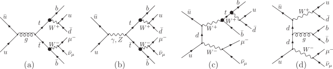
Figure 1: Examples of the lowest order Feynman diagrams of process (22). Black blobs indicate the $Wtb$ coupling.

Let us note that the $Wtb$ coupling that is indicated by a black blob enters twice both in the $t\bar{t}$ production signal diagrams depicted in Fig. 1a and 1b and the single top production diagram of Fig. 1c. Obviously it is not present in the off resonance background diagrams an example of which is shown in Fig. 1d. Needles to say that the by hand implementation of the anomalous $Wtb$ coupling in the matrix element of any of processes (21)–(22) would have been rather tedious a task. With the current version of carlomat the cross section of these processes can be computed automatically with any choice of the anomalous form factors of (16), as it was done in [11], where an influence of the anomalous $Wtb$ coupling on forward-backward asymmetry of top quark pair production at the Tevatron was investigated taking into account decays of the top quarks to 6 fermion final states containing one charged lepton.

4 Summary and Outlook

New developments in carlomat have been presented. They include improvements of the generation of phase space integration routines, implementation of scalar electrodynamics and the anomalous $Wtb$ coupling including operators of dimension up to five and many other improvements, as e.g., size reduction of the colour matrix, that have not been discussed in the present lecture. Some minor bugs in the program have been corrected too. A new version of the program will be released, hopefully soon.

Acknowledgements: This work was supported in part by the Research Executive Agency (REA) of the European Union under the Grant Agreement number PITN-GA-2010-264564 (LHCPhenoNet).

References

- [1] K. Kołodziej, Comput. Phys. Commun. 180 (2009) 1671.
- [2] K. Kołodziej, S. Szczypiński, Nucl. Phys. B801 (2008) 153 and Eur. Phys. J. C64 (2009) 645.
-
[3]
J.A. Aguilar-Saavedra et al. [ECFA/DESY LC Physics
Working Group Collaboration], arXiv:hep-ph/0106315;
T. Abe et al., [American Linear Collider Working Group Collaboration], arXiv:hep-ex/0106056;
K. Abe et al. [ACFA Linear Collider Working Group Collaboration], arXiv:hep-ph/0109166. -
[4]
R.W. Assmann et.al. [CLIC Study Team], CERN 2000–008;
H. Braun it et. al. [CLIC Study Group], CERN-OPEN-2008-021, CLIC-Note-764. - [5] G.L. Kane, G.A. Ladinsky, C.-P. Yuan, Phys. Rev. D45 (1992) 124.
- [6] K. Kołodziej, Phys. Lett. B584 (2004) 89.
- [7] D0 Collaboration, V.M. Abazov et al., Phys. Rev. Lett. 102 (2009) 092002.
- [8] J.A. Aguilar-Saavedra, N.F. Castro, A. Onofre, arXiv:1105.0117.
-
[9]
M.S. Alam et al., CLEO, Phys. Rev. Lett.
74, 2885 (1995);
F. Larios, M.A. Perez and C.-P. Yuan Phys. Lett. B457, 334 (1999). -
[10]
J. Drobnak, S. Fajfer, J.F. Kamenik, arXiv:1109.2357;
A. Crivellin, L. Mercolli, arXiv:1106.5499. - [11] K. Kołodziej, Phys. Lett. B710 (2012) 671.