Seven transiting hot-Jupiters from WASP-South, Euler and TRAPPIST: WASP-47b, WASP-55b, WASP-61b, WASP-62b, WASP-63b, WASP-66b & WASP-67b

Abstract

We present seven new transiting hot Jupiters from the WASP-South survey. The planets are all typical hot Jupiters orbiting stars from F4 to K0 with magnitudes of $V$ = 10.3 to 12.5. The orbital periods are all in the range 3.9–4.6 d, the planetary masses range from 0.4–2.3 M_Jup and the radii from 1.1–1.4 M_Jup. In line with known hot Jupiters, the planetary densities range from Jupiter-like to inflated ($\rho$ = 0.13–1.07 $\rho_{\rm Jup}$). We use the increasing numbers of known hot Jupiters to investigate the distribution of their orbital periods and the 3–4-d “pile-up”.

Table 1: Observations

Facility	Date
WASP-47:
WASP-South	2008 Jun–2010 Oct	18 300 points
Euler/CORALIE	2010 May–2011 Nov	19 radial velocities
EulerCAM	2011 Aug 02	Gunn r filter
WASP-55:
WASP-South	2006 May–2010 Jul	28 200 points
Euler/CORALIE	2011 Jan–2011 Jul	20 radial velocities
TRAPPIST	2011 Apr 04	$I+z$ filter
EulerCAM	2011 Jun 03	Gunn $r$ filter
TRAPPIST	2012 Jan 20	$I+z$ filter
WASP-61:
WASP-South	2006 Sep–2010 Feb	30 700 points
Euler/CORALIE	2011 Jan–2011 Nov	15 radial velocities
TRAPPIST	2011 Sep 09	Blue-block filter
EulerCAM	2011 Nov 16	Gunn $r$ filter
TRAPPIST	2011 Nov 16	Blue-block filter
TRAPPIST	2011 Dec 09	Blue-block filter
TRAPPIST	2011 Dec 13	Blue-block filter
WASP-62:
WASP-South	2008 Sep–2011 Feb	21 700 points
Euler/CORALIE	2011 Mar–2012 Apr	25 radial velocities
EulerCAM	2011 Nov 24	Gunn $r$ filter
TRAPPIST	2011 Dec 17	$z$-band filter
WASP-63:
WASP-South	2006 Oct–2010 Mar	24 700 points
Euler/CORALIE	2011 Feb–2012 Apr	23 radial velocities
TRAPPIST	2011 Dec 04	$z$-band filter
EulerCAM	2011 Dec 25	Gunn $r$ filter
EulerCAM	2012 Jan 29	Gunn $r$ filter
TRAPPIST	2012 Feb 21	$I+z$ filter
WASP-66:
WASP-South	2006 May–2011 Jun	19 600 points
Euler/CORALIE	2011 Jan–2012 Mar	30 radial velocities
TRAPPIST	2011 Apr 08	$I+z$ filter
TRAPPIST	2011 Dec 21	$I+z$ filter
TRAPPIST	2012 Mar 16	Blue-block filter
EulerCAM	2012 Mar 16	Gunn $r$ filter
WASP-67:
WASP-South	2006 May–2010 Sep	12 500 points
Euler/CORALIE	2011 Jul–2011 Oct	19 radial velocities
TRAPPIST	2011 Sep 29	$I+z$ filter
EulerCAM	2011 Sep 29	Gunn $r$ filter

1 Introduction

Transiting exoplanets found by the ground-based transit searches are mostly “hot Jupiters”, Jupiter-sized planets in $\approx$ 1–6-d orbits, since these are the easiest planets for such surveys to find. However, planet candidate lists from Kepler show that hot Jupiters are much less common than smaller planets (Batalha et al. 2012). This means that the much larger sky coverage of the ground-based surveys (e.g. WASP, Pollacco et al. 2006, and HATnet, Bakos et al. 2004) is needed to produce large samples of hot Jupiters that will enable us to understand the properties of this class. In addition, hot Jupiters from these surveys orbit stars of $V$ $\approx$ 9–13, which are bright enough for radial-velocity measurements of the planetary masses and for many other types of study.

Here we present seven new transiting planets discovered by the WASP-South survey (Hellier et al. 2011a) in conjunction with the Euler/CORALIE spectrograph and the TRAPPIST robotic photometer (Jehin et al. 2011). These are all hot Jupiters with $\sim$ 4-d orbits that are compatible with being circular, and with masses and radii that are typical of the class. They all orbit relatively isolated stars of $V$ = 10.3–12.5 which have metallicities and space velocities compatible with local thin-disc stars. WASP-South planets that are less typical of the class will be reported in other papers.

2 Observations

WASP-South uses an 8-camera array that covers 450 square degrees of sky observing with a typical cadence of 8 mins. The WASP surveys are described in Pollacco et al. (2006) while a discussion of our planet-hunting methods can be found in Collier-Cameron et al. (2007a) and Pollacco et al. (2007).

WASP-South planet candidates are followed up using the TRAPPIST robotic photometer and the CORALIE spectrograph on the Euler 1.2-m telescope at La Silla. About 1 in 12 candidates turns out to be a planet, the remainder being blends that are unresolved in the WASP data (which uses 14” pixels) or astrophysical transit mimics, usually eclipsing binary stars. A list of observations reported in this paper is given in Table 1 while the CORALIE radial velocities are listed in Table A1.

3 The host stars

The CORALIE spectra of the host stars were co-added to produce spectra for analysis using the methods described in Gillon et al. (2009). We used the H$\alpha$ line to determine the effective temperature ($T_{\rm eff}$), and the Na i D and Mg i b lines as diagnostics of the surface gravity ($\log g_{\rm*}$). The resulting parameters are listed in Tables 2 to 8. The elemental abundances were determined from equivalent-width measurements of several clean and unblended lines. A value for microturbulence ($\xi_{\rm t}$) was determined from Fe i lines using the criteria of a null-dependence of line abundances with equivalent width (see Magain 1984). The quoted error estimates include that given by the uncertainties in $T_{\rm eff}$, $\log g_{\rm*}$ and $\xi_{\rm t}$, as well as the scatter due to measurement and atomic data uncertainties.

The projected stellar rotation velocities ($v\sin I$) were determined by fitting the profiles of several unblended Fe i lines. We used values for macroturbulence ($v_{\rm mac}$) from the tabulation by Bruntt et al. (2010). A CORALIE instrumental FWHM of 0.11 $\pm$ 0.01 Å was determined from the telluric lines around 6300Å.

3.1 Rotational modulation

We searched the WASP photometry of each star for rotational modulations by using a sine-wave fitting algorithm as described by Maxted et al. (2011). We estimated the significance of periodicities by subtracting the fitted transit lightcurve and then repeatedly and randomly permuting the nights of observation. For none of our stars was a significant periodicity obtained, with 95%-confidence upper limits being typically 1 mmag (as listed in Tables 2 to 8).

3.2 Proper motions

For each of our stars we list (Tables 2 to 8) the proper motions from the UCAC3 catalogue (Zacharias et al. 2010). Combining these with the spectroscopic distances and the radial velocities in the same Tables gives space velocities in the range 19–55 km s^-1. Our stars are all compatible with the local thin-disc population, which typically has $-0.6<{\rm[Fe/H]}<0.3$ and $\sigma_{v}\approx 50$ km s^-1 (Navarro et al. 2011) .

4 System parameters

The CORALIE radial-velocity measurements were combined with the WASP, EulerCAM and TRAPPIST photometry in a simultaneous Markov-chain Monte-Carlo (MCMC) analysis to find the system parameters. For details of our methods see Collier Cameron et al. (2007b). The limb-darkening parameters are noted in each Table, and are taken from the 4-parameter non-linear law of Claret (2000).

For all of our planets the data are compatible with zero eccentricity and hence we imposed a circular orbit (see Anderson et al. 2012 for a discussion of the rationale for this). The fitted parameters were thus $T_{\rm c}$, $P$, $\Delta F$, $T_{14}$, $b$, $K_{\rm 1}$, where $T_{\rm c}$ is the epoch of mid-transit, $P$ is the orbital period, $\Delta F$ is the fractional flux-deficit that would be observed during transit in the absence of limb-darkening, $T_{14}$ is the total transit duration (from first to fourth contact), $b$ is the impact parameter of the planet’s path across the stellar disc, and $K_{\rm 1}$ is the stellar reflex velocity semi-amplitude.

The transit lightcurves lead directly to stellar density but one additional constraint is required to obtain stellar masses and radii, and hence full parametrisation of the system. We adopt the approach of Enoch et al. (2010), based on empirical calibrations of stellar properties from well-studied detached eclipsing binary systems, but we use the calibration coefficients calculated by Southworth (2011). These are improvements on the coefficients from Enoch et al. as they include far more stars (180 versus 38) and also restrict the calibration sample to objects with masses relevant to the study of transiting planetary systems (mass $<$ 3 M_⊙). The rms scatter of the calibrating sample around the best fit is 0.027 dex for log(mass) and 0.009 dex for log(radius).

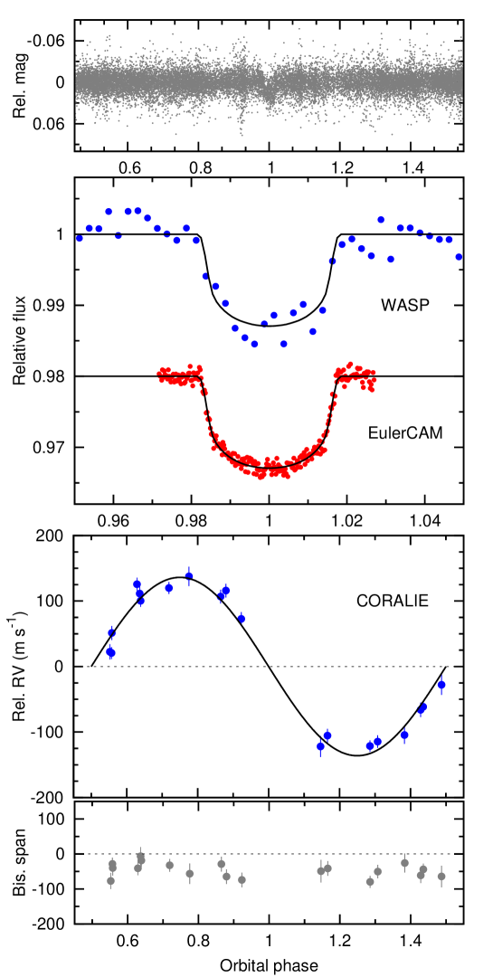
Figure 1: WASP-47b discovery data: (Top) The WASP-South lightcurve folded on the transit period. (Second panel) The binned WASP data with (offset) the follow-up transit lightcurves (ordered from the top as in Table 1) together with the fitted MCMC model. (Third) The CORALIE radial velocities with the fitted model. (Lowest) The bisector spans; the absence of any correlation with radial velocity is a check against transit mimics.

Table 2: System parameters for WASP-47.

1SWASP J220448.72–120107.8
2MASS 22044873–1201079
RA = 22h04m48.72s, Dec = –12∘01${}^{{}^{\prime}}$07.8${}^{{}^{\prime\prime}}$ (J2000)
$V$ mag = 11.9
Rotational modulation   $<$ 0.7 mmag (95%)
pm (RA) 17.1 $\pm$ 1.1 (Dec) –42.9 $\pm$ 1.0 mas/yr
Stellar parameters from spectroscopic analysis.
Spectral type	G9V
$T_{\rm eff}$ (K)	5400 $\pm$ 100
$\log g$	4.55 $\pm$ 0.10
$\xi_{\rm t}$ (km s-1)	0.7 $\pm$ 0.2
$v\,\sin I$ (km s-1)	3.0 $\pm$ 0.6
[Fe/H]	0.18 $\pm$ 0.07
[Na/H]	0.42 $\pm$ 0.06
[Mg/H]	0.21 $\pm$ 0.04
[Si/H]	0.36 $\pm$ 0.07
[Ca/H]	0.15 $\pm$ 0.11
[Ti/H]	0.28 $\pm$ 0.06
[Cr/H]	0.21 $\pm$ 0.10
[Ni/H]	0.30 $\pm$ 0.09
log A(Li)	$<$ 0.81 $\pm$ 0.10
Distance	200 $\pm$ 30 pc
Parameters from MCMC analysis.
$P$ (d)	4.1591399 $\pm$ 0.0000072
$T_{\rm c}$ (HJD) (UTC)	2455764.34602 $\pm$ 0.00022
$T_{\rm 14}$ (d)	0.14933 $\pm$ 0.00065
$T_{\rm 12}=T_{\rm 34}$ (d)	0.0141${}^{+0.0007}_{-0.0003}$
$\Delta F=R_{\rm P}^{2}$/R${}_{*}^{2}$	0.01051 $\pm$ 0.00014
$b$	0.14 $\pm$ 0.11
$i$ (∘)	89.2 ${}^{+0.5}_{-0.7}$
$K_{\rm 1}$ (km s-1)	0.136 $\pm$ 0.005
$\gamma$ (km s-1)	–27.056 $\pm$ 0.004
$e$	0 (adopted) ($<$0.11 at 3$\sigma$)
$M_{\rm*}$ (M⊙)	1.084 $\pm$ 0.037
$R_{\rm*}$ (R⊙)	1.15 ${}^{+0.03}_{-0.02}$
$\log g_{*}$ (cgs)	4.348${}^{+0.009}_{-0.016}$
$\rho_{\rm*}$ ($\rho_{\rm\odot}$)	0.71${}^{+0.02}_{-0.04}$
$T_{\rm eff}$ (K)	5350 $\pm$ 90
$M_{\rm P}$ (MJup)	1.14 $\pm$ 0.05
$R_{\rm P}$ (RJup)	1.15 ${}^{+0.04}_{-0.02}$
$\log g_{\rm P}$ (cgs)	3.29${}^{+0.02}_{-0.03}$
$\rho_{\rm P}$ ($\rho_{\rm J}$)	0.74${}^{+0.05}_{-0.06}$
$a$ (AU)	0.0520 $\pm$ 0.0006
$T_{\rm P,A=0}$ (K)	1220 $\pm$ 20
Errors are 1$\sigma$; Limb-darkening coefficients were:
(Euler $r$) a1 = 0.727, a2 = –0.653, a3 = 1.314, a4 = –0.594

For each system we list the resulting parameters in Tables 2 to 8, and plot the resulting data and models in Figures 1 to 7. We also refer the reader to Smith et al. (2012) who present an extensive analysis of the effect of red noise in the transit lightcurves on the resulting system parameters.

As in past WASP papers we plot the spectroscopic $T_{\rm eff}$, and the stellar density from fitting the transit, against the evolutionary tracks from Girardi et al. (2000), as shown in Fig. 8.

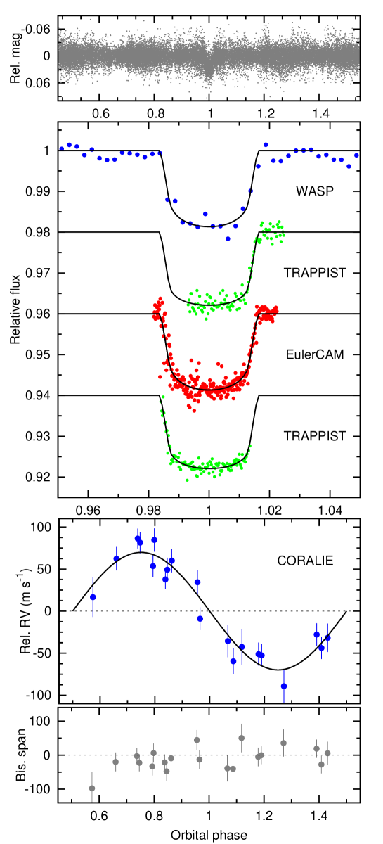
Figure 2: WASP-55b discovery data (as in Fig. 1).

Table 3: System parameters for WASP-55.

1SWASP J133501.94–173012.7
2MASS 13350194–1730124
TYCHO-2 6125-113-1
RA = 13h35m01.94s, Dec = –17∘30${}^{{}^{\prime}}$12.7${}^{{}^{\prime\prime}}$ (J2000)
$V$ mag = 11.8
Rotational modulation   $<$ 1 mmag (95%)
pm (RA) 11.2 $\pm$ 1.0 (Dec) –8.2 $\pm$ 1.0 mas/yr
Stellar parameters from spectroscopic analysis.
Spectral type	G1
$T_{\rm eff}$ (K)	5900 $\pm$ 100
$\log g$	4.3 $\pm$ 0.1
$\xi_{\rm t}$ (km s-1)	1.1 $\pm$ 0.1
$v\,\sin I$ (km s-1)	3.1 $\pm$ 1.0
[Fe/H]	$-$0.20 $\pm$ 0.08
[Na/H]	$-$0.21 $\pm$ 0.05
[Mg/H]	$-$0.17 $\pm$ 0.04
[Si/H]	$-$0.13 $\pm$ 0.05
[Ca/H]	$-$0.10 $\pm$ 0.10
[Sc/H]	$-$0.05 $\pm$ 0.08
[Ti/H]	$-$0.08 $\pm$ 0.05
[Cr/H]	$-$0.18 $\pm$ 0.07
[Ni/H]	$-$0.21 $\pm$ 0.06
$\log A$(Li)	2.36 $\pm$ 0.09
Distance	330 $\pm$ 50 pc
Parameters from MCMC analysis.
$P$ (d)	4.465633 $\pm$ 0.000004
$T_{\rm c}$ (HJD) (UTC)	2455737.9396 $\pm$ 0.0003
$T_{\rm 14}$ (d)	0.147 $\pm$ 0.001
$T_{\rm 12}=T_{\rm 34}$ (d)	0.0167${}^{+0.0011}_{-0.0004}$
$\Delta F=R_{\rm P}^{2}$/R${}_{*}^{2}$	0.0158 $\pm$ 0.0003
$b$	0.15 $\pm$ 0.12
$i$ (∘)	89.2 $\pm$ 0.6
$K_{\rm 1}$ (km s-1)	0.070 $\pm$ 0.004
$\gamma$ (km s-1)	–4.3244 $\pm$ 0.0009
$e$	0 (adopted) ($<$0.20 at 3$\sigma$)
$M_{\rm*}$ (M⊙)	1.01 $\pm$ 0.04
$R_{\rm*}$ (R⊙)	1.06${}^{+0.03}_{-0.02}$
$\log g_{*}$ (cgs)	4.39${}^{+0.01}_{-0.02}$
$\rho_{\rm*}$ ($\rho_{\rm\odot}$)	0.85${}^{+0.03}_{-0.07}$
$T_{\rm eff}$ (K)	5960 $\pm$ 100
$M_{\rm P}$ (MJup)	0.57 $\pm$ 0.04
$R_{\rm P}$ (RJup)	1.30${}^{+0.05}_{-0.03}$
$\log g_{\rm P}$ (cgs)	2.89 $\pm$ 0.04
$\rho_{\rm P}$ ($\rho_{\rm J}$)	0.26${}^{+0.02}_{-0.03}$
$a$ (AU)	0.0533 $\pm$ 0.0007
$T_{\rm P,A=0}$ (K)	1290 $\pm$ 25
Errors are 1$\sigma$; Limb-darkening coefficients were:
(Euler $r$) a1 = 0.496, a2 = 0.201, a3 = 0.183, a4 = –0.170
(Trapp $Iz$) a1 = 0.587, a2 = –0.180, a3 = 0.441, a4 = –0.250

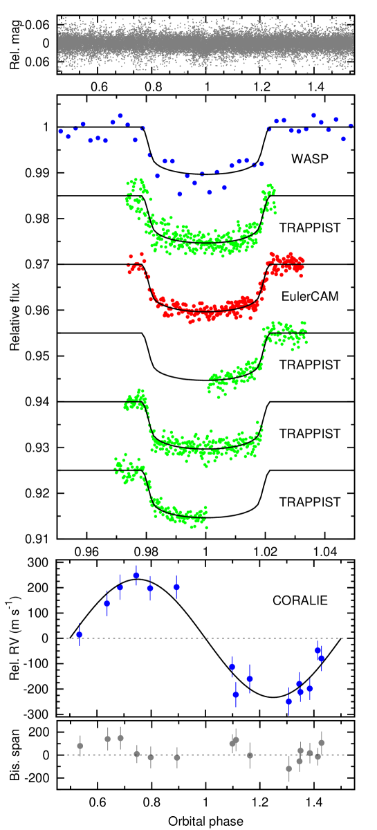
Figure 3: WASP-61b discovery data (as in Fig. 1).

Table 4: System parameters for WASP-61.

1SWASP J050111.91–260314.9
2MASS 05011191–2603149
TYCHO-2 6469-1972-1
RA = 05h01m11.91s, Dec = –26∘03${}^{{}^{\prime}}$14.9${}^{{}^{\prime\prime}}$ (J2000)
$V$ mag = 12.5
Rotational modulation   $<$ 1.5 mmag (95%)
pm (RA) 1.0 $\pm$ 0.9 (Dec) 0.5 $\pm$ 1.0 mas/yr
Stellar parameters from spectroscopic analysis.
Spectral type	F7
$T_{\rm eff}$ (K)	6250 $\pm$ 150
$\log g$	4.3 $\pm$ 0.1
$\xi_{\rm t}$ (km s-1)	1.0 $\pm$ 0.2
$v\,\sin I$ (km s-1)	10.3 $\pm$ 0.5
[Fe/H]	–0.10 $\pm$ 0.12
log A(Li)	$<$ 1.13 $\pm$ 0.11
Distance	480 $\pm$ 65 pc
Parameters from MCMC analysis.
$P$ (d)	3.855900 $\pm$ 0.000003
$T_{\rm c}$ (HJD) (UTC)	2455859.52825 $\pm$ 0.00023
$T_{\rm 14}$ (d)	0.1642 $\pm$ 0.0006
$T_{\rm 12}=T_{\rm 34}$ (d)	0.0142${}^{+0.0004}_{-0.0002}$
$\Delta F=R_{\rm P}^{2}$/R${}_{*}^{2}$	0.0088 $\pm$ 0.0001
$b$	0.09${}^{+0.09}_{-0.06}$
$i$ (∘)	89.35${}^{+0.45}_{-0.66}$
$K_{\rm 1}$ (km s-1)	0.233 $\pm$ 0.016
$\gamma$ (km s-1)	18.970 $\pm$ 0.002
$e$	0 (adopted) ($<$0.26 at 3$\sigma$)
$M_{\rm*}$ (M⊙)	1.22 $\pm$ 0.07
$R_{\rm*}$ (R⊙)	1.36 $\pm$ 0.03
$\log g_{*}$ (cgs)	4.256 $\pm$ 0.011
$\rho_{\rm*}$ ($\rho_{\rm\odot}$)	0.487${}^{+0.008}_{-0.017}$
$T_{\rm eff}$ (K)	6320 $\pm$ 140
$M_{\rm P}$ (MJup)	2.06 $\pm$ 0.17
$R_{\rm P}$ (RJup)	1.24 $\pm$ 0.03
$\log g_{\rm P}$ (cgs)	3.48 $\pm$ 0.03
$\rho_{\rm P}$ ($\rho_{\rm J}$)	1.07 $\pm$ 0.09
$a$ (AU)	0.0514 $\pm$ 0.0009
$T_{\rm P,A=0}$ (K)	1565 $\pm$ 35
Errors are 1$\sigma$; Limb-darkening coefficients were:
(All) a1 = 0.466, a2 = 0.414, a3 = –0.192, a4 = 0.002

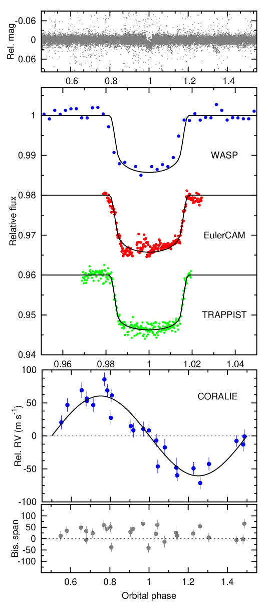
Figure 4: WASP-62b discovery data (as in Fig. 1).

Table 5: System parameters for WASP-62.

1SWASP J054833.59–635918.3
2MASS 05483359–6359183
TYCHO-2 8900-874-1
RA = 05h48m33.59s, Dec = –63∘59${}^{{}^{\prime}}$18.3${}^{{}^{\prime\prime}}$ (J2000)
$V$ mag = 10.3
Rotational modulation   $<$ 1 mmag (95%)
pm (RA) –14.0 $\pm$ 0.9 (Dec) –27.0 $\pm$ 1.0 mas/yr
Stellar parameters from spectroscopic analysis.
Spectral type	F7
$T_{\rm eff}$ (K)	6230 $\pm$ 80
$\log g$	4.45 $\pm$ 0.10
$\xi_{\rm t}$ (km s-1)	1.25 $\pm$ 0.10
$v\,\sin I$ (km s-1)	8.7 $\pm$ 0.4
[Fe/H]	0.04 $\pm$ 0.06
[Na/H]	$-$0.02 $\pm$ 0.03
[Mg/H]	0.07 $\pm$ 0.08
[Al/H]	0.03 $\pm$ 0.03
[Si/H]	0.11 $\pm$ 0.08
[Ca/H]	0.16 $\pm$ 0.12
[Sc/H]	0.10 $\pm$ 0.05
[Ti/H]	0.11 $\pm$ 0.08
[V/H]	0.01 $\pm$ 0.09
[Cr/H]	0.09 $\pm$ 0.07
[Mn/H]	$-$0.08 $\pm$ 0.05
[Co/H]	$-$0.02 $\pm$ 0.10
[Ni/H]	0.04 $\pm$ 0.08
$\log A$(Li)	2.48 $\pm$ 0.06
Distance	160 $\pm$ 30 pc
Parameters from MCMC analysis.
$P$ (d)	4.411953 $\pm$ 0.000003
$T_{\rm c}$ (HJD) (UTC)	2455855.39195 $\pm$ 0.00027
$T_{\rm 14}$ (d)	0.1588 $\pm$ 0.0014
$T_{\rm 12}=T_{\rm 34}$ (d)	0.0172 $\pm$ 0.0012
$\Delta F=R_{\rm P}^{2}$/R${}_{*}^{2}$	0.0123 $\pm$ 0.0002
$b$	0.29${}^{+0.08}_{-0.14}$
$i$ (∘)	88.3${}^{+0.9}_{-0.6}$
$K_{\rm 1}$ (km s-1)	0.060 $\pm$ 0.004
$\gamma$ (km s-1)	14.970 $\pm$ 0.005
$e$	0 (adopted) ($<$ 0.21 at 3$\sigma$)
$M_{\rm*}$ (M⊙)	1.25 $\pm$ 0.05
$R_{\rm*}$ (R⊙)	1.28 $\pm$ 0.05
$\log g_{*}$ (cgs)	4.316 $\pm$ 0.025
$\rho_{\rm*}$ ($\rho_{\rm\odot}$)	0.59 $\pm$0.06
$T_{\rm eff}$ (K)	6280 $\pm$ 80
$M_{\rm P}$ (MJup)	0.57 $\pm$ 0.04
$R_{\rm P}$ (RJup)	1.39 $\pm$ 0.06
$\log g_{\rm P}$ (cgs)	2.83 $\pm$ 0.04
$\rho_{\rm P}$ ($\rho_{\rm J}$)	0.21 $\pm$ 0.03
$a$ (AU)	0.0567 $\pm$ 0.0007
$T_{\rm P,A=0}$ (K)	1440 $\pm$ 30
Errors are 1$\sigma$; Limb-darkening coefficients were:
(Euler $r$) a1 = 0.508, a2 = 0.269, a3 = 0.015, a4 = –0.090
(Trapp $Iz$) a1 = 0.585, a2 = –0.095, a3 = 0.276, a4 = –0.176

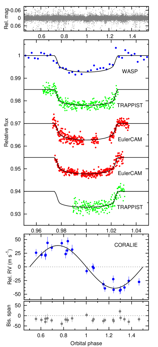
Figure 5: WASP-63b discovery data (as in Fig. 1).

Table 6: System parameters for WASP-63.

1SWASP J061720.74–381923.8
2MASS 06172074–3819237
TYCHO-2 7612-556-1
RA = 06h17m20.74s, Dec = –38∘19${}^{{}^{\prime}}$23.8${}^{{}^{\prime\prime}}$ (J2000)
$V$ mag = 11.2
Rotational modulation   $<$ 0.8 mmag (95%)
pm (RA) –16.5 $\pm$ 0.9 (Dec) –26.7 $\pm$ 0.9 mas/yr
Stellar parameters from spectroscopic analysis.
Spectral type	G8
$T_{\rm eff}$ (K)	5550 $\pm$ 100
$\log g$	3.9 $\pm$ 0.1
$\xi_{\rm t}$ (km s-1)	0.9 $\pm$ 0.1
$v\,\sin I$ (km s-1)	2.8 $\pm$ 0.5
[Fe/H]	0.08 $\pm$ 0.07
[Na/H]	0.18 $\pm$ 0.06
[Mg/H]	0.20 $\pm$ 0.05
[Si/H]	0.24 $\pm$ 0.05
[Ca/H]	0.18 $\pm$ 0.13
[Sc/H]	0.09 $\pm$ 0.11
[Ti/H]	0.12 $\pm$ 0.06
[V/H]	0.16 $\pm$ 0.11
[Cr/H]	0.10 $\pm$ 0.04
[Co/H]	0.14 $\pm$ 0.06
[Ni/H]	0.15 $\pm$ 0.05
$\log A$(Li)	$<$ 0.96 $\pm$ 0.10
Distance	330 $\pm$ 50 pc
Parameters from MCMC analysis.
$P$ (d)	4.378090 $\pm$ 0.000006
$T_{\rm c}$ (HJD) (UTC)	2455921.6527 $\pm$ 0.0005
$T_{\rm 14}$ (d)	0.2225 $\pm$ 0.0017
$T_{\rm 12}=T_{\rm 34}$ (d)	0.017${}^{+0.002}_{-0.001}$
$\Delta F=R_{\rm P}^{2}$/R${}_{*}^{2}$	0.00609 $\pm$ 0.00017
$b$	0.26${}^{+0.13}_{-0.15}$
$i$ (∘)	87.8 $\pm$ 1.3
$K_{\rm 1}$ (km s-1)	0.039 $\pm$ 0.003
$\gamma$ (km s-1)	–23.712 $\pm$ 0.003
$e$	0 (adopted) ($<$ 0.22 at 3$\sigma$)
$M_{\rm*}$ (M⊙)	1.32 $\pm$ 0.05
$R_{\rm*}$ (R⊙)	1.88${}^{+0.10}_{-0.06}$
$\log g_{*}$ (cgs)	4.01${}^{+0.02}_{-0.04}$
$\rho_{\rm*}$ ($\rho_{\rm\odot}$)	0.198${}^{+0.017}_{-0.025}$
$T_{\rm eff}$ (K)	5570 $\pm$ 90
$M_{\rm P}$ (MJup)	0.38 $\pm$ 0.03
$R_{\rm P}$ (RJup)	1.43${}^{+0.10}_{-0.06}$
$\log g_{\rm P}$ (cgs)	2.62 $\pm$ 0.05
$\rho_{\rm P}$ ($\rho_{\rm J}$)	0.13 $\pm$ 0.02
$a$ (AU)	0.0574 $\pm$ 0.0007
$T_{\rm P,A=0}$ (K)	1540 $\pm$ 40
Errors are 1$\sigma$; Limb-darkening coefficients were:
(Euler $r$) a1 = 0.679, a2 = –0.433, a3 = 1.017, a4 = –0.494
(Trapp $Iz$) a1 = 0.766, a2 = –0.688, a3 = 1.056, a4 = –0.479

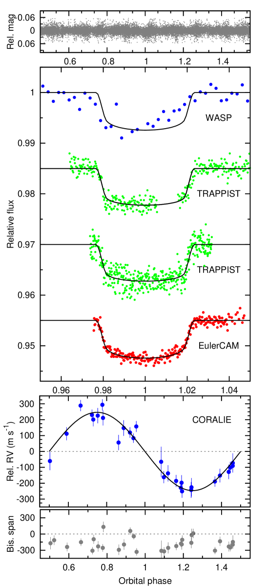
Figure 6: WASP-66b discovery data (as in Fig. 1); the two parts of the upper TRAPPIST curve were taken on different nights.

Table 7: System parameters for WASP-66.

1SWASP J103254.00–345923.3
2MASS 10325399–3459234
TYCHO-2 7193-1804-1
RA = 10h32m54.00s, Dec = –34∘59${}^{{}^{\prime}}$23.3${}^{{}^{\prime\prime}}$ (J2000)
$V$ mag = 11.6
Rotational modulation   $<$ 1 mmag
pm (RA) 11.0 $\pm$ 0.8 (Dec) –13.1 $\pm$ 0.8 mas/yr
Stellar parameters from spectroscopic analysis.
Spectral type	F4
$T_{\rm eff}$ (K)	6600 $\pm$ 150
$\log g$	4.3 $\pm$ 0.2
$\xi_{\rm t}$ (km s-1)	2.2 $\pm$ 0.3
$v\,\sin I$ (km s-1)	13.4 $\pm$ 0.9
[Fe/H]	$-$0.31 $\pm$ 0.10
[Na/H]	$-$0.29 $\pm$ 0.06
[Mg/H]	$-$0.27 $\pm$ 0.10
[Si/H]	$-$0.19 $\pm$ 0.06
[Ca/H]	$-$0.19 $\pm$ 0.10
[Sc/H]	$-$0.17 $\pm$ 0.12
[Ti/H]	$-$0.16 $\pm$ 0.15
[V/H]	$-$0.10 $\pm$ 0.11
[Cr/H]	$-$0.25 $\pm$ 0.15
[Mn/H]	$-$0.37 $\pm$ 0.12
[Co/H]	$-$0.15 $\pm$ 0.08
[Ni/H]	$-$0.38 $\pm$ 0.10
$\log A$(Li)[LTE]	3.06 $\pm$ 0.11
$\log A$(Li)[N-LTE]	2.97 $\pm$ 0.11
Distance	380 $\pm$ 100 pc
Parameters from MCMC analysis.
$P$ (d)	4.086052 $\pm$ 0.000007
$T_{\rm c}$ (HJD) (UTC)	2455929.09615 $\pm$ 0.00035
$T_{\rm 14}$ (d)	0.1876 $\pm$ 0.0017
$T_{\rm 12}=T_{\rm 34}$ (d)	0.018 $\pm$ 0.002
$\Delta F=R_{\rm P}^{2}$/R${}_{*}^{2}$	0.00668 $\pm$ 0.00016
$b$	0.48${}^{+0.06}_{-0.08}$
$i$ (∘)	85.9 $\pm$ 0.9
$K_{\rm 1}$ (km s-1)	0.246 $\pm$ 0.011
$\gamma$ (km s-1)	–10.02458 $\pm$ 0.00013
$e$	0 (adopted) ($<$ 0.11 at 3$\sigma$)
$M_{\rm*}$ (M⊙)	1.30 $\pm$ 0.07
$R_{\rm*}$ (R⊙)	1.75 $\pm$ 0.09
$\log g_{*}$ (cgs)	4.06 $\pm$ 0.04
$\rho_{\rm*}$ ($\rho_{\rm\odot}$)	0.242${}^{+0.036}_{-0.028}$
$T_{\rm eff}$ (K)	6580 $\pm$ 170
$M_{\rm P}$ (MJup)	2.32 $\pm$ 0.13
$R_{\rm P}$ (RJup)	1.39 $\pm$ 0.09
$\log g_{\rm P}$ (cgs)	3.44 $\pm$ 0.05
$\rho_{\rm P}$ ($\rho_{\rm J}$)	0.860${}^{+0.17}_{-0.13}$
$a$ (AU)	0.0546 $\pm$ 0.0009
$T_{\rm P,A=0}$ (K)	1790 $\pm$ 60
Errors are 1$\sigma$; Limb-darkening coefficients were:
(Euler $r$) a1 = 0.353, a2 = 0.759, a3 = –0.628, a4 = 0.177
(Trapp $Iz$) a1 = 0.443, a2 = 0.299, a3 = –0.213, a4 = 0.022

Figure 7: WASP-67b discovery data (as in Fig. 1).

Table 8: System parameters for WASP-67.

1SWASP J194258.51–195658.4
2MASS 19425852–1956585
TYCHO-2 6307-1388-1
RA = 19h42m58.51s, Dec = –19∘56${}^{{}^{\prime}}$58.4${}^{{}^{\prime\prime}}$ (J2000)
$V$ mag = 12.5
Rotational modulation   $<$ 3 mmag
pm (RA) 0.7 $\pm$ 1.3 (Dec) –33.8 $\pm$ 2.4 mas/yr
Stellar parameters from spectroscopic analysis.
Spectral type	K0V
$T_{\rm eff}$ (K)	5200 $\pm$ 100
$\log g$	4.35 $\pm$ 0.15
$\xi_{\rm t}$ (km s-1)	0.9 $\pm$ 0.1
$v\,\sin I$ (km s-1)	2.1 $\pm$ 0.4
[Fe/H]	$-$0.07 $\pm$ 0.09
[Na/H]	0.11 $\pm$ 0.08
[Mg/H]	0.05 $\pm$ 0.04
[Si/H]	0.15 $\pm$ 0.03
[Ca/H]	0.02 $\pm$ 0.12
[Ti/H]	0.01 $\pm$ 0.06
[V/H]	0.09 $\pm$ 0.08
[Cr/H]	0.06 $\pm$ 0.03
[Co/H]	0.05 $\pm$ 0.04
[Ni/H]	0.00 $\pm$ 0.08
$\log A$(Li)	$<$ 0.23 $\pm$ 0.11
Distance	225 $\pm$ 45 pc
Parameters from MCMC analysis.
$P$ (d)	4.61442 $\pm$ 0.00001
$T_{\rm c}$ (HJD) (UTC)	2455824.3742 $\pm$ 0.0002
$T_{\rm 14}$ (d)	0.079 $\pm$ 0.001
$\Delta F=R_{\rm P}^{2}$/R${}_{*}^{2}$	0.0181${}^{+0.0013}_{-0.0005}$
$b$	0.94${}^{+0.05}_{-0.03}$
$i$ (∘)	85.8${}^{+0.3}_{-0.4}$
$K_{\rm 1}$ (km s-1)	0.056 $\pm$ 0.004
$\gamma$ (km s-1)	–0.5634 $\pm$ 0.0002
$e$	0 (adopted) ($<$0.20 at 3$\sigma$)
$M_{\rm*}$ (M⊙)	0.87 $\pm$ 0.04
$R_{\rm*}$ (R⊙)	0.87 $\pm$ 0.04
$\log g_{*}$ (cgs)	4.50 $\pm$ 0.03
$\rho_{\rm*}$ ($\rho_{\rm\odot}$)	1.32 $\pm$ 0.15
$T_{\rm eff}$ (K)	5240 $\pm$ 10
$M_{\rm P}$ (MJup)	0.42 $\pm$ 0.04
$R_{\rm P}$ (RJup)	1.4 ${}^{+0.3}_{-0.2}$
$\log g_{\rm P}$ (cgs)	2.7${}^{+0.1}_{-0.2}$
$\rho_{\rm P}$ ($\rho_{\rm J}$)	0.16 $\pm$ 0.08
$a$ (AU)	0.0517 $\pm$ 0.0008
$T_{\rm P,A=0}$ (K)	1040 $\pm$ 30
Errors are 1$\sigma$; Limb-darkening coefficients were:
(Euler $r$) a1 = 0.671, a2 = –0.540, a3 = 1.225, a4 = –0.574
(Trapp $Iz$) a1 = 0.744, a2 = –0.707, a3 = 1.134, a4 = –0.506

5 WASP-47

WASP-47 is a G9 star ($V$ = 11.9) with a possibly elevated metallicity of [Fe/H] = 0.18 $\pm$ 0.07. There is no significant detection of lithium in the spectra, with an equivalent width upper limit of 3mÅ, corresponding to an abundance upper limit of $\log A$(Li) $<$ 0.81 $\pm$ 0.10. The temperature of 5400K along with the lithium abundance imply a lower age limit of around 0.6 Gyr when compared with the Hyades cluster (Sestito & Randlich 2005). The rotation rate ($P=15\pm 3$ d) implied by the $v\sin I$ (assuming that the planet’s orbit is aligned, and thus that the star’s spin axis is perpendicular to us) gives a gyrochronological age of $\sim 1.0^{+0.7}_{-0.4}$ Gyr using the Barnes (2007) relation.

With an orbital period of 4.16 d, a mass of 1.14 M_Jup and a radius of 1.15 R_Jup WASP-47b is an entirely typical hot Jupiter.

6 WASP-55

WASP-55 is a G1 star ($V$ = 11.8) with a below-solar metallicity of [Fe/H] = –0.20 $\pm$ 0.07. The lithium abundance in WASP-55 implies an age of $\ga$ 2 Gyr (Sestito & Randlich 2005). The rotation rate ($P=20\pm 7$ d) implied by the $v\sin I$ gives a gyrochronological age of $\sim 3^{+5}_{-2}$ Gyr using the Barnes (2007) relation.

2MASS images of WASP-55 show a star approximately 2^′′ away and about 5 magnitudes fainter. This is sufficiently faint that it is unlikely to be affecting our results significantly.

WASP-55b is moderately inflated, with a mass of 0.57 M_Jup and a radius of 1.30 R_Jup, though this is in line with many known hot Jupiters.

7 WASP-61

WASP-61 is an F7 star ($V$ = 12.5) with metallicity near solar (the poor quality of our spectrum prevents more detailed analysis than the [Fe/H] = –0.10 $\pm$ 0.12 reported in Table 4). There is no significant detection of lithium in the spectra, corresponding to an abundance upper limit of $\log A$(Li) $<$ 1.1 $\pm$ 0.1, which implies an age of several Gyr (Sestito & Randlich 2005). The rotation rate ($P=6.3\pm 0.9$ d) implied by the $v\sin I$ gives a gyrochronological age of $\sim 0.7^{+1.2}_{-0.4}$ Gyr using the Barnes (2007) relation.

WASP-61b has a high mass of $M$ = 2.1 M_Jup and the highest density of the planets reported here, at $\rho$ = 1.1 $\rho$_Jup.

8 WASP-62

WASP-62 is an F7 star ($V$ = 10.3) with a solar metallicity. For a star of this temperature (6230 $\pm$ 80 K) the presence of relatively strong lithium absorption in the spectrum does not provide a strong age constraint; this level of depletion is found in clusters as young as $\sim$0.5 Gyr (Sestito & Randlich 2005). The rotation rate ($P=6.3\pm 0.8$ d) implied by the $v\sin I$ gives a gyrochronological age of $\sim 0.7^{+0.4}_{-0.3}$ Gy using the Barnes (2007) relation. There are no emission peaks evident in the Ca ii H+K lines.

The EulerCAM transit lightcurve is badly affected by weather. Our MCMC analysis balances $\chi^{2}$ across the different datasets, so inflates the error bars of this lightcurve. We also ran the analysis omitting this curve, which led to results that were the same within the errors.

9 WASP-63

WASP-63 is a G8 star ($V$ = 11.2) with solar metallicity. There is no significant detection of lithium in the spectra, with an equivalent width upper limit of 11mÅ, corresponding to an abundance upper limit of $\log A$(Li) $<$ 0.96 $\pm$ 0.10. This implies an age of at least several Gyr (Sestito & Randlich 2005). The rotation rate ($P=37\pm 9$ d) implied by the $v\sin I$ gives a gyrochronological age of $\sim 6^{+5}_{-3}$ Gyr using the Barnes (2007) relation. There are no emission peaks evident in the Ca ii H+K lines.

The stellar radius is inflated for a G8 star and indicates that WASP-63 has evolved off the main sequence (see Fig. 8), with an age of $\sim$ 8 Gyr.

The planet WASP-63b is the least massive of those reported here, at 0.38 M_Jup, and also has the lowest density ($\rho$ = 0.13 $\rho$_Jup). This indicates that mechanisms causing inflated planet radii need to be able to operate late on in the evolution of a planetary system.

10 WASP-66

WASP-66 is an F4 star ($V$ = 11.6) with a below-solar metallicity of [Fe/H] = –0.31 $\pm$ 0.10. With $T_{\rm eff}$ = 6600 $\pm$ 150 K WASP-66 is relatively hot among known hot-Jupiter hosts. The presence of strong lithium absorption in the spectrum suggests that WASP-66 is $\la$2 Gyr old (Sestito & Randlich 2005). The rotation rate ($P=4.9\pm 1.3$ d) implied by the $v\sin I$ gives little age constraint, $3.3^{+10}_{-2.7}$ Gyr, from the Barnes (2007) relation.

With a mass of 2.3 M_Jup WASP-66b is the most massive of the planets reported here.

11 WASP-67

WASP-67 is an K0V star ($V$ = 12.5) with a solar metallicity. There is no significant detection of lithium in the spectra, with an equivalent width upper limit of 5mÅ, corresponding to an abundance upper limit of $\log A$(Li) $<$ 0.23 $\pm$ 0.11. This implies an age of at least $\sim$0.5 Gyr (Sestito & Randlich 2005). The rotation rate ($P=25\pm 7$ d) implied by the $v\sin I$ gives a gyrochronological age of $2.0^{+1.6}_{-1.0}$ Gyr using the Barnes (2007) relation. There are no emission peaks evident in the Ca ii H+K lines.

WASP-67b has a mass of 0.42 M_Jup and a radius of 1.4 M_Jup, making it inflated ($\rho$ = 0.16 $\rho$_Jup). It also has a high impact factor of $b=0.94$, making the transit curve V-shaped. If the criterion $X=b+R_{\rm P}/R_{*}>1$ is satisfied then the transit is grazing, with part of the planet not transiting the stellar face (see, e.g., Smalley et al. 2011). For WASP-67b this value is 1.07${}^{+0.05}_{-0.03}$, and, further, out of 375 000 MCMC steps only 17 had $X<1$. This implies a $>$3$\sigma$ probability that the transit is grazing, making WASP-67b the first hot Jupiter known to have a grazing transit, following WASP-34 and HAT-P-27/WASP-40 that are possibly grazing (Smalley et al. 2011; Anderson et al. 2011).

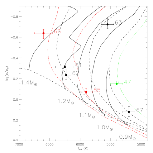
Figure 8: Evolutionary tracks on a modified H–R diagram ($\rho_{*}^{-1/3}$ versus $T_{\rm eff}$). The black lines are for solar metallicity, [Fe/H] = 0, showing (solid lines) mass tracks with the labelled masses, and (dashed lines) age tracks for $\log$(age) = 7.8, 9.4, 9.9 & 10.2 yrs. The four host stars with near-solar metallicities are shown in black. The green-labelled WASP-47 has above-solar metallicity of [Fe/H] = +0.18, and the green dotted line is the age track for [Fe/H] = +0.18 and $\log$(age) = 10.2 yrs. The red dot-dashed lines are for a below-solar metallicity of [Fe/H] = –0.2, being at ages $\log$(age) = 9.4 & 9.8 yrs. The two host stars with below-solar metallicities are labelled in red. The data are from Girardi et al. (2000).

12 Discussion

It has often been noted that the hot-Jupiter population shows an apparent “pile up” at orbital periods of $P$ = 3–4 d. We can use the increasing numbers of hot Jupiters, primarily from the ground-based transit surveys, to investigate this.

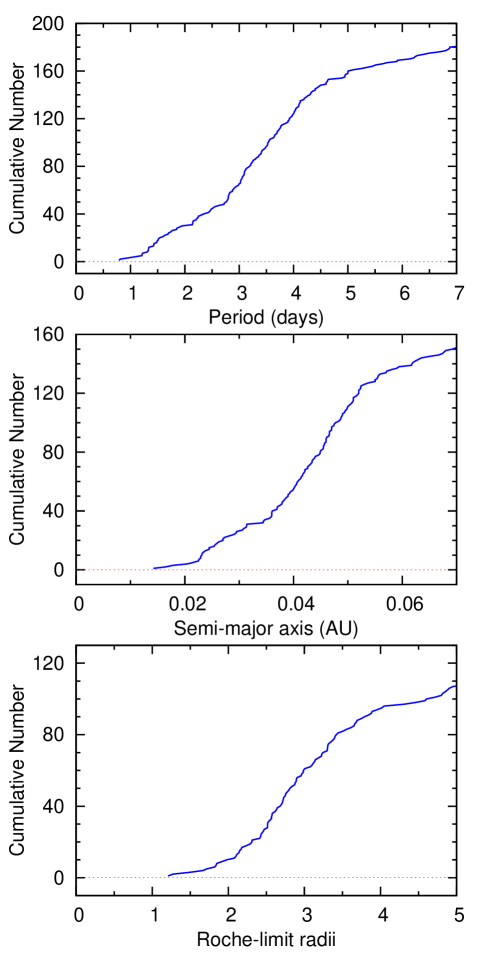
Figure 9: The cumulative distributions of (top) orbital period, (middle) semi-major axis, and (bottom) separations in units of Roche-limit separation for a sample of hot Jupiters (see text). The definition of Roche-limit separation is taken from Ford & Rasio (2006).

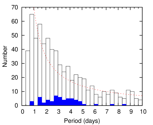
Figure 10: The open histogram shows the period distribution of all WASP-South candidates that have been rejected or confirmed as planets. The solid histogram shows the planets. The dotted line is a simple $P^{-1}$ function, scaling as the number of transits observed in a WASP-like survey.

As a first step we take the sample of confirmed planets compiled by Schneider et al. (2011), as of March 2012, limiting this to periods less than 8 days and planetary masses of 0.1–12 M_Jup (the super-Earths may well be a different population dynamically). We show (Fig. 9) the cumulative distributions against orbital period, semi-major axis and Roche-limit separation. These confirm that we see more planets at periods $P$ of $\approx$ 3–5 days, with fewer at shorter and longer periods. However, this compilation comes from many different surveys, each of which will have different selection effects, and so needs to be interpreted with caution.

We thus create a second sample of planets discovered by the transit surveys ($P<8$ d, $M$ = 0.1–12 M_Jup), based on the Schneider et al. compilation but with unpublished WASP planets added up to WASP-84b. This sample of 163 planets is dominated by WASP (81 planets), HAT (34), Kepler (18) and CoRoT (14).

The inclination range that produces a transit scales with semi-major axis as $\cos^{-1}(R_{*}/a)$. To compare this with the distribution of orbital periods, which are securely known, we can translate this to $P$ by assuming a star of solar mass and radius. Further, the biggest factor affecting discovery probability in a WASP-like survey is the number of transits recorded, which will scale as $P^{-1}$. In Fig. 10 we show the distribution of rejected WASP-South candidates, which indicates that a $P^{-1}$ function, though imperfect, is a rough approximation.

We caution that this is only a very preliminary account of relevant selection effects, which will be different for each of the above surveys. For example, the number of transits required is likely to saturate above some number (this number depending on the survey and the amount of data), and WASP-like surveys at only one longitude will also suffer from sampling effects at integer-day periods.

Nevertheless, we can multiply together the transit probability and the $P^{-1}$ function to produce the detection-probability curve shown in Fig. 11, and we can use this to produce a “corrected” planet distribution curve.

One can interpret this curve as showing four regions with different slopes, the slopes having relative ratios (for corrected number of planets versus period interval) of 1 : 10 : 40 : 12. The need for different slopes in the different regions is significant on a K–S test at $>$95% probabilities. We caution, though, that we regard this as an indicative description of the distribution, rather than a unique one, and the relative slopes are of course dependent on the uncertain selection effects.

The four regions of the hot-Jupiter period distribution are:

(1) $P$ = 0.8–1.2 d, containing only 4 planets (WASP-19b, WASP-43b, WASP-18b & WASP-12b; Hebb et al. 2010; Hellier et al. 2011b; Hellier et al. 2009; Hebb et al. 2009), despite the probability of detection being greatest. These planets are thought to be tidally decaying on relatively short timescales, and so are rare, found only by the surveys sampling the most stars (see the discussion in Hellier et al. 2011b; note that WASP observes from one longitude with greater sky coverage than HATnet, whereas HATnet covers less sky but from several longitudes).

There are no known hot Jupiters with a period below the $P$ = 0.79-d of WASP-19b. Despite the fact that the probability of detection of such planets in WASP data is at its highest (see Fig. 11 curve), the number of good candidates declines (Fig. 10), and, further, we have followed up over 40 such candidates without success (compared to an overall success rate of 1-in-12). Thus hot-Jupiter planets below $P$ = 0.79-d must be very rare (there are several super-Earths with such periods, though their tidal-decay rate will of course be much lower).

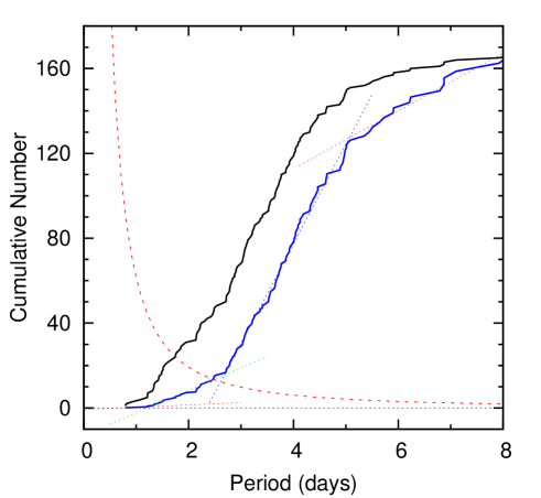
Figure 11: The solid-black line is the cumulative distribution of orbital periods for transiting hot Jupiters. The solid-blue line is the same but corrected for the probability of detection (which is the dotted curve). The dotted straight lines are a suggested parametrisation of the distribution (see text).

(2) $P$ = 1.2–2.7 d. The abundance is an order of magnitude greater than in the 0.8–1.2 d range, but still a factor $\sim$ 4 lower than in the range 2.7–5-d.

(3) $P$ = 2.7–5-d. Our analysis confirms the existence of a pile-up of hot Jupiters, and suggests that it has a relatively well defined lower edge at $P$ = 2.7-d.

Ford & Rasio (2006) argued that a hot-Jupiter population resulting from circularisation of highly eccentric orbits will have an inner edge at 2 Roche-limit radii (2$a_{R}$ where $a_{R}=\frac{R_{P}}{0.462}\left(\frac{M_{P}}{M_{*}}\right)^{1/3}$).

For a planet of Jupiter mass and radius around a star of solar mass and radius, 2 $a_{R}$ corresponds to $P$ = 1.2-d, and so would explain our finding of a break at that period. The few systems inside that limit are presumably spiralling inward relatively rapidly under tidal decay (e.g.  Matsumura, Peale & Rasio 2010).

Further, for an inflated planet with a radius of $R\approx 1.8$ R_Jup (as seen in the highly inflated planets WASP-12b, WASP-17b, HAT-P-32b & HAT-P-33b; Hebb et al. 2009; Anderson et al. 2010; Hartman et al. 2011) 2 $a_{R}$ equates to $P$ = 2.7 d (again assuming a 1-M_Jup planet orbiting a sun-like star). Hence, if hot Jupiters arrive in the pile-up with a range of radius inflations, the Ford & Rasio argument would produce a cut-off ranging from $\sim$ 1.2 to 2.7 d, which might explain our finding of breaks at both those values.

(4) $P$ = $\sim$ $>$ 5-d. The upper edge of the pile-up appears to be near 5-d, although we caution that in WASP-like surveys the detection probability (and hence number of planets) decreases, and the selection effects get worse, as the period increases beyond $P$ $\sim$ 5 d. For this reason we don’t further interpret the longer-period range.

The period distribution of hot Jupiters is likely to result from several physical mechanisms. These include disk migration and possible ‘stopping mechanisms’ (e.g. Matsumura, Pudritz & Thommes 2007), third-body interactions, such as the Kozai mechanism, that can move planets onto highly eccentric orbits that are then tidally captured and circularise at short periods (e.g. Guillochon et al. 2011; Noaz et al. 2011), and orbital decay and in-spiral caused by tidal interactions with the host star (e.g. Matsumura et al. 2010).

Study of the angle between the planetary orbit and the stellar rotation axis indicates that many current orbits are likely to result from the Kozai mechanism (e.g. Triaud et al. 2010), but it is probable that the hot Jupiters are a composite population with differing past histories. Thus, to further investigate the pile-up, we need to accumulate statistics to look for differences in, for example, the orbital eccentricities and the spin–orbit angle between the different period ranges that we have outlined.

Appendix A Online only

Table 9: CORALIE radial velocities.

BJD – 2400 000	RV	$\sigma$RV	Bisector
(UTC)	(km s-1)	(km s-1)	(km s-1)
WASP-47:
55328.9147	$-$27.199	0.010	$-$0.050
55384.9303	$-$26.943	0.015	$-$0.056
55389.7034	$-$27.008	0.010	$-$0.074
55390.7133	$-$27.186	0.011	$-$0.041
55391.8362	$-$27.142	0.008	$-$0.044
55392.6807	$-$26.980	0.009	$-$0.019
55396.7987	$-$26.954	0.010	$-$0.041
55403.6889	$-$27.201	0.009	$-$0.080
55408.6869	$-$27.107	0.015	$-$0.064
55409.6504	$-$26.959	0.009	$-$0.032
55450.5481	$-$27.054	0.012	$-$0.077
55454.7270	$-$27.055	0.009	$-$0.029
55782.7653	$-$27.121	0.011	$-$0.061
55795.7802	$-$27.003	0.011	$-$0.040
55809.5958	$-$26.937	0.011	$-$0.065
55885.5702	$-$27.170	0.016	$-$0.049
55886.5550	$-$27.153	0.014	$-$0.026
55887.6093	$-$26.937	0.013	$-$0.007
55888.5579	$-$26.941	0.011	$-$0.029
WASP-55:
55591.7843	$-$4.414	0.020	0.036
55593.8655	$-$4.238	0.012	$-$0.003
55595.8370	$-$4.375	0.014	$-$0.005
55596.7857	$-$4.352	0.013	0.019
55598.7838	$-$4.287	0.012	$-$0.021
55599.8011	$-$4.360	0.019	$-$0.039
55602.8371	$-$4.243	0.013	$-$0.022
55604.8196	$-$4.377	0.013	$-$0.000
55605.7954	$-$4.368	0.013	$-$0.028
55607.7461	$-$4.275	0.014	$-$0.047
55623.7577	$-$4.356	0.017	0.006
55624.7801	$-$4.262	0.014	$-$0.020
55625.6823	$-$4.264	0.014	$-$0.009
55629.8416	$-$4.271	0.013	$-$0.033
55635.7567	$-$4.367	0.021	0.050
55637.7936	$-$4.308	0.024	$-$0.097
55665.5870	$-$4.240	0.014	0.006
55675.8082	$-$4.384	0.016	$-$0.040
55679.7306	$-$4.333	0.014	$-$0.013
55764.5358	$-$4.290	0.015	0.044
WASP-61:
55570.7149	18.857	0.041	0.099
55615.6221	19.218	0.039	0.009
55629.5093	18.790	0.046	$-$0.054
55649.5172	18.985	0.045	0.080
55650.5243	19.168	0.048	$-$0.020
55802.8748	18.721	0.056	$-$0.120
55806.8968	18.758	0.039	0.038
55809.8327	18.748	0.049	0.132
55810.8849	18.772	0.045	0.017
55811.8571	19.108	0.050	0.140
55813.8869	18.810	0.057	$-$0.004
55814.9060	18.891	0.050	0.106
55815.8979	19.172	0.049	0.148
55839.8379	19.172	0.046	$-$0.024
55868.8371	18.923	0.038	$-$0.015
Bisector errors are twice RV errors

Table 9: continued

BJD – 2400 000	RV	$\sigma$RV	Bisector
(UTC)	(km s-1)	(km s-1)	(km s-1)
WASP-62:
55651.4898	15.039	0.009	0.043
55675.4985	14.921	0.010	0.022
55676.4710	14.963	0.009	–0.006
55677.4992	15.023	0.009	–0.005
55678.4947	14.985	0.010	0.030
55681.4724	15.017	0.010	0.035
55682.4765	15.032	0.010	–0.038
55683.4807	14.963	0.010	0.020
55684.4733	14.899	0.009	0.054
55685.4723	14.969	0.011	0.066
55692.4975	14.953	0.013	–0.013
55693.4947	14.928	0.010	0.005
55809.8571	15.027	0.012	0.033
55810.9091	14.979	0.011	0.042
55811.8813	14.922	0.015	0.026
55815.8730	14.924	0.010	0.061
55836.8736	14.998	0.010	0.050
55839.8625	14.957	0.010	–0.003
55840.8861	15.017	0.010	0.024
55850.8434	14.981	0.011	0.065
55864.8453	14.910	0.009	0.012
55881.8528	14.979	0.010	–0.041
55888.6963	14.991	0.011	0.012
55889.6691	15.056	0.010	0.059
56021.5148	15.039	0.012	0.048
WASP-63:
55598.7288	–23.771	0.006	–0.026
55649.4954	–23.679	0.007	–0.022
55651.5371	–23.768	0.007	–0.011
55670.5213	–23.705	0.006	–0.030
55675.5315	–23.682	0.007	–0.040
55676.4936	–23.733	0.006	0.003
55677.5218	–23.747	0.007	–0.021
55678.5172	–23.752	0.007	–0.018
55679.5209	–23.690	0.006	–0.023
55681.5178	–23.756	0.007	–0.026
55682.4989	–23.750	0.008	–0.030
55683.5030	–23.703	0.007	–0.020
55684.4956	–23.695	0.007	–0.020
55685.5179	–23.727	0.007	–0.017
55695.4660	–23.762	0.007	–0.017
55802.8982	–23.687	0.009	–0.013
55805.8813	–23.692	0.007	–0.016
55836.8931	–23.694	0.010	–0.015
55858.8607	–23.671	0.011	–0.013
55869.8341	–23.754	0.006	–0.022
55895.6363	–23.713	0.007	–0.024
55966.7350	–23.752	0.007	0.021
56021.5498	–23.683	0.008	–0.019
Bisector errors are twice RV errors

Table 9: continued

BJD – 2400 000	RV	$\sigma$RV	Bisector
(UTC)	(km s-1)	(km s-1)	(km s-1)
WASP-66:
55572.7155	–9.813	0.048	0.131
55623.6364	–10.250	0.059	–0.019
55627.7156	–10.267	0.050	–0.163
55628.7858	–10.085	0.057	–0.170
55629.7107	–9.824	0.043	–0.096
55632.6904	–10.097	0.061	–0.148
55635.6818	–10.222	0.048	–0.192
55643.5642	–10.162	0.051	–0.257
55644.6746	–10.177	0.043	–0.135
55646.7038	–9.877	0.049	–0.195
55647.5623	–10.186	0.038	–0.322
55648.6521	–10.214	0.033	–0.307
55649.5716	–9.913	0.041	–0.240
55650.6813	–9.968	0.048	0.292
55651.5910	–10.089	0.095	–0.311
55674.6304	–9.794	0.034	–0.310
55675.5760	–9.867	0.034	–0.331
55676.5274	–10.254	0.033	–0.179
55677.6348	–10.115	0.037	–0.196
55679.6014	–9.941	0.030	–0.043
55680.6394	–10.276	0.041	–0.108
55681.6674	–10.126	0.036	–0.250
55682.5584	–9.736	0.035	–0.152
55683.6124	–9.905	0.033	0.055
55684.5982	–10.210	0.038	–0.223
55707.5410	–9.731	0.035	–0.257
55711.5280	–9.799	0.048	–0.229
55722.4965	–10.153	0.046	–0.232
55958.7274	–10.388	0.044	0.012
56000.6947	–9.983	0.045	–0.115
WASP-67:
55765.7296	$-$0.610	0.013	0.028
55767.7027	$-$0.507	0.015	0.019
55768.6736	$-$0.544	0.011	0.027
55769.6850	$-$0.613	0.011	0.030
55770.7119	$-$0.610	0.013	$-$0.015
55777.7996	$-$0.511	0.014	0.029
55793.5324	$-$0.605	0.017	$-$0.017
55794.5285	$-$0.548	0.017	0.017
55795.5247	$-$0.528	0.014	0.020
55798.5058	$-$0.586	0.026	$-$0.006
55803.5145	$-$0.567	0.018	$-$0.052
55804.5425	$-$0.495	0.013	$-$0.009
55805.4867	$-$0.532	0.012	0.010
55806.6210	$-$0.600	0.015	0.001
55807.6815	$-$0.607	0.014	0.018
55819.5305	$-$0.540	0.010	0.017
55820.5790	$-$0.626	0.010	$-$0.004
55826.5015	$-$0.570	0.014	$-$0.026
55851.5050	$-$0.548	0.013	$-$0.009
Bisector errors are twice RV errors

References

- [Anderson et al. (2010)] Anderson D. R. et al., 2010, ApJ, 709, 159
- [Anderson et al. (2011)] Anderson D. R. et al., 2011, PASP, 123, 555
- [Anderson et al. (2012)] Anderson D. R. et al., 2012, MNRAS, in press (arXiv1105.3179)
- [Bakos et al.(2004)] Bakos G. À., Noyes R. W., Kovács G., Stanek K. Z., Sasselov, D. D., Domsa, I., PASP, 116, 266
- [Barnes (2007)] Barnes, S.A. 2007, ApJ, 669, 1167
- [Batalha et al. (2012)] Batalha N. M. et al., 2012, ApJS submitted (arXiv1202.5852)
- [Bruntt et al. (2010)] Bruntt, H. et al., 2010, MNRAS, 405, 1907
- [Claret (2000)] Claret, A., 2000, A&A, 363, 1081
- [Collier Cameron et al.(2007a)] Collier Cameron, A., et al., 2007a, MNRAS, 375, 951
- [Collier Cameron et al.(2007b)] Collier Cameron, A., et al., 2007b, MNRAS, 380, 1230
- [Enoch et al. (2010)] Enoch B., Collier Cameron A., Parley N. R., Hebb L., 2010, A&A, 516, A33
- [Ford & Rasio (2006)] Ford, E. B. & Rasio, F. A., 2006, ApJ, 638, L45
- [Gillon et al. (2007)] Gillon, M., et al., 2009, A&A, 496, 259
- [1] Girardi, L., Bressan, A., Bertelli, G., Chiosi, C. 2000, A&AS, 141, 371
- [Guillochon et al. (2011)] Guillochon, J., Ramirez-Ruiz, E., Lin, D. N. C., 2011, ApJ, 732, 74
- [Hebb et al. (2009)] Hebb, L. et al., 2009, ApJ, 693, 1920
- [Hebb et al. (2010)] Hebb, L. et al., 2010, ApJ, 708, 224
- [Hellier et al. (2009)] Hellier, C. et al., 2009, Nature, 460, 1098
- [Hellier et al. (2011a)] Hellier, C. et al., 2011a, in “Detection and dynamics of transiting exoplanets”, eds F. Bouchy, R. Díaz, C. Moutou, EPJ Web of Conferences, Volume 11, id.01004
- [Hellier et al. (2011b)] Hellier, C. et al., 2011b, A&A, 535, L7
- [Jehin et al. (2011)] Jehin, E. et al., 2011, Messenger, 145, 2
- [2] Matsumura, S., Pudritz, R.E.. Thommes, E.W. 2007, ApJ, 660, 1609
- [Matsumura et al. (2010)] Matsumura, S., Peale, S. J., Rasio, F. A., 2010, ApJ, 725, 1995
- [3] Maxted, P.F.L. et al. 2011, PASP, 123, 547
- [4] Naoz, S., Farr, W. M., Lithwick, Y., Rasio, F. A., Teyssandier, J., 2011, Nature, 473, 187
- [5] Navarro J. F., Abadi M. G.. Venn, K. A., Freeman K. C., Anguiano B., 2011, MNRAS, 412, 1203
- [Magain (1984)] Magain, P., 1984, A&A, 134, 189
- [Pollacco et al. (2006)] Pollacco, D., et al., 2006, PASP, 118, 1407
- [Pollacco et al. (2007)] Pollacco, D., et al., 2008, MNRAS, 385, 1576
- [Schneider et al. (2011)] Schneider, J, Dedieu, C., Le Sidaner, P., Savalle, R., Zolotukhin, I., 2011, A&A, 532, A79
- [Sestito & Randlich (2005)] Sestito, P. & Randlich, S., 2005, A&A, 442, 615
- [Smalley et al. (2011)] Smalley B. et al. 2011, A&A, 526, 130
- [Smith et al. (2012)] Smith A. M. S. et al. 2012, AJ, 143, 81
- [Southworth] Southworth J., 2011, MNRAS, 417, 2166
- [Triaud et al. (2010)] Triaud, A. H. M. J., 2010, A&A, 524, 25
- [6] Zacharias, N. et al. 2010, AJ, 139, 2184