De Sitter-spacetime instability from a nonstandard vector field

Abstract

It is found that de Sitter spacetime, the constant-curvature matter-free solution of the Einstein equations with a positive cosmological constant, becomes classically unstable due to the dynamic effects of a certain type of vector field (fundamentally different from a gauge field). The perturbed de Sitter universe evolves towards a final singularity. The relevant vector-field configurations violate the strong and dominant energy conditions.

I Introduction

The Einstein gravitational field equations with positive cosmological constant Einstein1917 have a highly symmetric matter-free solution, de Sitter spacetime deSitter1917 ; HawkingEllis1973 . Nearly a century after the discovery of this mathematical solution, de Sitter spacetime occupies a central place in modern theoretical physics and observational cosmology (see, for example, the reviews Weinberg1989 ; PDG2010 ). It is, then, all the more interesting if something new can be said about de Sitter spacetime, even if the context is nonstandard.

In recent work on the cosmological constant problem, we noted parenthetically (Footnote 1 in Appendix A of Ref. EmelyanovKlinkhamer2011-CCP1-FRW-NEWTON ) that, for the simple model considered, de Sitter spacetime corresponded to an unstable critical point. The simple model considered Dolgov1997 ; EmelyanovKlinkhamer2011-CCP1-NEWTON had a classical vector field $V_{\alpha}(x)$ with a “wrong-sign” kinetic term [giving energy density $\rho_{\text{vec}}\leq 0$ for the cosmological solution], which we suspected to be responsible for the de Sitter instability. It will, however, be shown in the present article that the de Sitter instability is also present in the model with a “correct-sign” kinetic term [giving $\rho_{\text{vec}}\geq 0$ for the cosmological solution].

The particular type of vector-field theory considered (Sec. II) is, most likely, pathological, having instabilities at the classical level and ghosts at the quantum level. Still, the vector field interacts only gravitationally with the other matter fields. As such, this classical vector field may be used to describe certain nonstandard gravitational effects in the long-wavelength (low-energy) limit. Two examples of such effects are discussed in the present article, namely, a particular type of instability of the de Sitter equilibrium solution (Sec. III) and the corresponding final singularity (Sec. IV). The estimated de Sitter decay time and the violation of certain energy conditions by the relevant vector-field configurations are discussed in Sec. V. In that last section, it is also explained how this type of classical vector field can perhaps play a role in the macroscopic description of a fundamental quantum instability of de Sitter spacetime Polyakov2007 ; Polyakov2009 ; KrotovPolyakov2010 .

II Theory

Consider general relativity with a positive cosmological constant $\Lambda$ and a single classical vector field $V_{\alpha}(x)$. The specific gravitational model Dolgov1997 ; EmelyanovKlinkhamer2011-CCP1-FRW-NEWTON ; EmelyanovKlinkhamer2011-CCP1-NEWTON used here has the following action ($c=\hbar=1$):

$$S[g,\,V,\,\phi] = -\int\,d^{4}x\,\sqrt{-\text{det}(g)}\,\bigg{(}\frac{1}{2}\,(E_{\text{Planck}})^{2}\,R[g]+\epsilon\big{(}Q_{1}[g,\,V]\big{)}+\Lambda+\mathcal{L}_{M}[g,\,\phi]\bigg{)},$$ (1a)

$$\epsilon\big{(}Q_{1}[g,\,V]\big{)} = -\big{(}Q_{1}[g,\,V]\big{)}^{2}\equiv-V_{\alpha;\beta}\,V^{\alpha;\beta}\,,$$ (1b)

$$E_{\text{Planck}} \equiv (8\pi G)^{-1/2}\,,\quad G>0\,,\quad\Lambda>0\,,$$ (1c)

where a generic massless matter field $\phi(x)$ has been added with a standard Lagrange density $\mathcal{L}_{M}(x)$. The action (1a) is really classical, but, for convenience, we use quantum terminology such as $E_{\text{Planck}}$. In principle, it is also possible to add a mass term for the vector field, but we refrain from doing so for the moment and the theory maintains the shift invariance of the vector field.

Notice that, unlike the case of a gauge field with a Maxwell action-density term, the time derivative of the $V_{0}$ component enters the action-density term (1b). It is, of course, known that, in Minkowski spacetime ($\Lambda=0$), gauge invariance is required for the Poincaré invariance, locality, and stability of the massless-vector-field theory Weinberg1964 . However, as explained in Sec. I, our interest in the classical massless vector field from (1) is only as an effective way to describe possible nonstandard gravitational effects related to the cosmological constant $\Lambda>0$. Our focus will be on stability issues in a cosmological context.

Let us restrict our attention to the spatially flat ($k=0$) Robertson–Walker metric HawkingEllis1973 with a perfect-fluid standard-matter component and an isotropic vector field (vanishing spatial components in appropriate coordinates). The dimensionless ordinary differential equations (ODEs) are then

$$3\,h^{2}=1+\dot{v}^{2}+3\,h^{2}\,v^{2}+\lambda^{-1}\,r_{M}\,\,,$$ (2a)

$$2\,\dot{h}=2\,\dot{h}\,v^{2}+4\,h\,v\,\dot{v}-2\,\dot{v}^{2}-\lambda^{-1}\,(1+w_{M})\,r_{M}\,,$$ (2b)

$$\ddot{v}+3\,h\,\dot{v}-3\,h^{2}\,v=0\,,$$ (2c)

$$\dot{r}_{M}+3\,(1+w_{M})\,h\,r_{M}=0\,,$$ (2d)

where a numerical factor $\sqrt{\lambda}\equiv\sqrt{\Lambda}/(E_{\text{Planck}})^{2}>0$ has been absorbed into the definitions of the dimensionless inverse Hubble parameter $h^{-1}$ and the dimensionless cosmic time $\tau$ (the overdot stands for differentiation with respect to this $\tau$). The dimensionless variable $v$ corresponds to the vector-field time-component $V_{0}$ and the dimensionless variable $r_{M}\geq 0$ corresponds to the standard-matter energy density $\rho_{M}\geq 0$ with constant equation-of-state parameter $w_{M}\geq 0$. See Appendix A of Ref. EmelyanovKlinkhamer2011-CCP1-FRW-NEWTON for further details.

Using Eq. (A6) from Ref. EmelyanovKlinkhamer2011-CCP1-NEWTON , the corresponding dimensionless vector-field energy density $r_{\text{vec}}$ and pressure $p_{\text{vec}}$ are found to be given by

$$r_{\text{vec}} \equiv e(q_{1})-q_{1}\,\frac{de(q_{1})}{dq_{1}}=+(q_{1})^{2}=\lambda\,(\dot{v}^{2}+3\,h^{2}\,v^{2})\geq 0\,,$$ (3a)

$$p_{\text{vec}} = -r_{\text{vec}}-2\,\lambda\,\big{(}\dot{h}\,v^{2}+2\,h\,v\,\dot{v}-\dot{v}^{2}\big{)}\,,$$ (3b)

parts of which, divided by $\lambda$, can be seen to appear on the right-hand sides of (2a) and (2b). Remark that, in a Minkowski background with $H=\Lambda=0$, the vector-field fluid (3) is not unusual, it corresponds to a matter component with an ultrahard equation of state, $\rho_{\text{vec}}=P_{\text{vec}}=(dV_{0}/dt)^{2}\geq 0$. What is unusual is how the vector-field pressure (3b) behaves in a nonflat spacetime background, possibly having $P_{\text{vec}}<-\rho_{\text{vec}}<0$.

III Unstable equilibrium

The ODEs (2) have an asymptotic equilibrium solution (critical point) corresponding to de Sitter spacetime:

$$1/h(\tau) = \sqrt{3}\,,$$ (4a)

$$v(\tau) = 0\,,$$ (4b)

$$r_{M}(\tau) = 0\,.$$ (4c)

There are no asymptotic solutions with $h\sim 0$, which would approach Minkowski spacetime EmelyanovKlinkhamer2011-CCP1-FRW-NEWTON ; Dolgov1997 ; EmelyanovKlinkhamer2011-CCP1-NEWTON . The explanation is that, with the minus sign chosen in (1b), the cosmological constant cannot be canceled by the vector-field contribution, as the right-hand side of (2a) makes clear ($\lambda^{-1}\,r_{M}$ is non-negative).

The equilibrium solution (4) is, however, unstable. We will show this numerically, but it can also be proven mathematically by following the discussion in Appendix A of Ref. EmelyanovKlinkhamer2011-CCP1-FRW-NEWTON (in fact, the linearized analysis suffices, according to Theorem 3.2 of Ref. Verhulst1996 ).

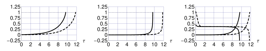
Figure 1: Numerical solutions of ODEs (2b) and (2c) with dimensionless cosmological constant $\lambda>0$ and vanishing standard-matter component, $r_{M}(\tau)=0$. The left panel shows the dimensionless vector-field component $v(\tau)$. The middle panel shows $(3\,h^{2})^{-1}\,\dot{v}^{2}/(1-v^{2})$. The right panel shows $r_{\text{vec}}/(3\,\lambda\,h^{2})$ as the ascending curves and $3/4+(1/4)\,(p_{\text{vec}}/r_{\text{vec}})$ as the descending curves. The vector-field boundary conditions are $v(0)=1/130$ and $\dot{v}(0)=\pm 1/130$, where the solid and dashed curves correspond to the plus and minus sign, respectively. The values for $h(0)$ follow from (2a) [both curves have, in fact, the same value of $h(0)$]. The Hubble parameter $h(\tau)$ and the vector-field energy density $r_{\text{vec}}(\tau)$ diverge at $\tau\approx 9.635$ for the $\dot{v}(0)>0$ boundary condition (ascending solid curve of the right panel) and at $\tau\approx 11.794$ for the $\dot{v}(0)<0$ boundary condition (ascending dashed curve of the right panel).

Numerical solutions have been obtained with vanishing and nonvanishing standard-matter components. For the case of a nonvanishing standard-matter component, it is found that an asymptotic de Sitter spacetime is approached if the vector field is strictly equal to zero, but not if the vector field is nonzero. As the conclusion is essentially the same for the case of a vanishing standard-matter component, we focus on the $r_{M}=0$ case endnote:rMnonzero . Instead of reaching an asymptotic de Sitter spacetime, the model universe of Fig. 1 is seen to terminate after a finite time interval, having a diverging Ricci scalar $R\propto-6\,(\dot{h}+2\,h^{2})$ at $\tau\sim 10$. The same type of behavior as shown in Fig. 1 is obtained for boundary conditions taking values in the finite intervals $v(0)\in(0,\,1/100]$ and $\dot{v}(0)\in[-1/100,\,+1/100]$.

Hence, we have established numerically the classical instability of de Sitter spacetime (4) under vector-field perturbations $\delta v(\tau)$ which break the original de Sitter symmetry. We have, in addition, explicit analytic results for the linear perturbations but will not present them here, as the numerical results suffice to demonstrate the instability.

IV Final singularity

The numerical results of the previous section suggest that the model universe of Fig. 1 runs into a final singularity (also known as a big-rip-type future singularity or, more generally, as an exotic future singularity, see Refs. Caldwell1999 ; Starobinsky1999 ; McInnes2001 ; Caldwell-etal2003 ; Faraoni2003 ; Nojiri-etal2005 ; Dabrowski2011 ; Barrow-etal2012 and references therein). Some analytic results have been obtained for the vector-field theory (1) with vanishing standard-matter component, $r_{M}(\tau)=0$. The pure vector-field theory considered here is of interest, because it has a strictly non-negative energy density (3a), different from the scalar-field theory with a negative quartic coupling constant as discussed in Ref. Faraoni2003 .

The ODEs (2) now reduce to

$$\ddot{v}+3\,h\,\dot{v}-3\,h^{2}\,v = 0\,,$$ (5a)

$$\big{(}\dot{h}\big{)}^{-1}-\left(\frac{2\,h\,v\,\dot{v}-\dot{v}^{2}}{1-v^{2}}\right)^{-1} = 0\,,$$ (5b)

$$\frac{h^{-2}+h^{-2}\,\dot{v}^{2}}{3\,(1-v^{2})} = 1\,\,,$$ (5c)

where $h$, $\dot{h}$, and $1-v^{2}$ are assumed to be nonzero. Next, make a change of variable $s=\ln(a)$ for cosmic scale factor $a(\tau)$, with $a(0)=1$ and Hubble parameter $h\equiv\dot{a}/a\equiv ds/d\tau$. The following ODEs for $v(s)$ and $h(s)$ are found:

$$v^{\prime\prime}+\frac{2\,v-v^{\prime}}{1-v^{2}}\,(v^{\prime})^{2}+3\,(v^{\prime}-v) = 0\,,$$ (6a)

$$\big{(}h^{\prime}\big{)}^{-1}-\left(\frac{2\,v-v^{\prime}}{1-v^{2}}\,v^{\prime}\,h\right)^{-1} = 0\,,$$ (6b)

$$\frac{h^{-2}+(v^{\prime})^{2}}{3\,(1-v^{2})} = 1\,\,,$$ (6c)

where the prime stands for differentiation with respect to $s$. There are only two arbitrary constants of integration as the last two ODEs in (6) are first-order (the first ODE is consistent with the last two ODEs; cf. Sec. III A of Ref. EmelyanovKlinkhamer2011-CCP1-FRW-NEWTON ).

It is easy to check that a particular combination of trigonometric functions solves the nonlinear ODE (6a). With an arbitrary real amplitude $A\in[-1,\,+1]$ and an arbitrary relative sign entering the solution for $v(s)$ and with a nonzero real amplitude $B$ in $h(s)$, the following solutions of the ODEs (6a) and (6b) are obtained:

$$v(s) = A\,\sin\big{(}\sqrt{3}\,s\big{)}\pm\sqrt{1-A^{2}}\,\cos\big{(}\sqrt{3}\,s\big{)}\,,$$ (7a)

$$1/h(s) = B\,\big{[}1+(2A^{2}-1)\cos(2\sqrt{3}\,s)\mp 2A\,\sqrt{1-A^{2}}\,\sin(2\sqrt{3}\,s)\big{]}\,\exp(3\,s)\,.$$ (7b)

A consistent solution of the differential system (6) with $v$ and $h$ given by (7a) and (7b) requires a solution of the constraint (6c). From (7a), this implies $h^{-2}=0$, which is only possible for special values of $s$ according to (7b). It turns out that $|v|=1$ for the values of $s$ that nullify $1/h$. One concrete example has $A=1$ and $s=\pi/(2\sqrt{3})$, while keeping an arbitrary nonzero $B$. Specifically, we have for this particular critical point of the differential system (6):

$$\Big{[}1/h(s)\,\Big{]}_{s=\pi/(2\sqrt{3})} = \Big{[}B\,\big{[}1+\cos(2\sqrt{3}\,s)\big{]}\,e^{3\,s}\,\Big{]}_{s=\pi/(2\sqrt{3})}=0\,,$$ (8a)

$$\Big{[}v(s)\,\Big{]}_{s=\pi/(2\sqrt{3})} = \Big{[}\sin\big{(}\sqrt{3}\,s\big{)}\,\Big{]}_{s=\pi/(2\sqrt{3})}=1\,.$$ (8b)

The actual value for $s$ at the critical point is nonphysical (because $a$ is); what matters is that, for example, the Ricci scalar diverges there. For cosmic times just before the singularity, the functions $v$ and $1/h$ can be expected to be slightly different from those given in (7).

Moreover, the following corollary can be obtained from (6c):

$$\left[\frac{1}{3}\;\frac{(v^{\prime})^{2}}{1-v^{2}}\,\right]_{\text{singularity}}=1\,,$$ (9a)

where the suffix is interpreted as being arbitrarily close to the point with $$1/h(s)=d\tau/ds=0$$ corresponding to (8a). The explicit solution (7a) can also be seen to satisfy (9a). In turn, (9a) gives for the vector-field energy density (3a) the following result:

$$\left[\frac{r_{\text{vec}}}{3\,\lambda\,h^{2}}\,\right]_{\text{singularity}}=\left[\frac{\rho_{\text{vec}}}{3\,(E_{\text{Planck}})^{2}\,H^{2}}\,\right]_{\text{singularity}}=1\,,$$ (9b)

with dimensional quantities in the middle expression. A final characteristic concerns the diverging vector-field equation-of-state parameter $$w_{\text{vec}}\equiv p_{\text{vec}}/r_{\text{vec}}$$ and can be stated as follows:

$$\left[\sqrt{3\,(1-v^{2})/16}\;\;\frac{r_{\text{vec}}+p_{\text{vec}}}{r_{\text{vec}}}\,\right]_{\text{singularity}}=-1\,,$$ (9c)

which, using (9b), can also be written with $3\,\lambda\,h^{2}$ in the denominator.

Further mathematical discussion of the final singularity (8) is left to a future publication. Note that, strictly speaking, the qualification “final” is arbitrary, as the tensor-vector-scalar theory (1) is time-reversal-invariant and so is the differential system (5).

For the present article, the relevant observation is that the numerical results of Fig. 1 can be interpreted as interpolating between the critical points (4) and (8). Indeed, the particular combination $3^{-1}\,h^{-2}\,(\dot{v})^{2}/(1-v^{2})$ from the middle panel of Fig. 1 is seen to run between the values $0$ and $1$, which are the corresponding values from (4) and (9a). The numerical results for the ratio $r_{\text{vec}}/(3\,\lambda\,h^{2})$ from the right panel of Fig. 1 show the same behavior, running between the values $0$ and $1$ from (4) and (9b), respectively. Numerical results also match (9c), but have not been shown explicitly in Fig. 1.

Including standard-matter, the final singularity is characterized by having $\rho_{\text{vec}}/\Lambda\to\infty$ and $\rho_{M}/\Lambda\to\text{const}>0$, in addition to having a diverging Ricci scalar $R$ as mentioned before. This exotic behavior, just as that of Fig. 1 for the $\rho_{M}=0$ case, is, most likely, the result of the unusual properties of the vector-field energy density and pressure, which will be discussed in the next section.

V Discussion

Let us, first, elaborate on the remark of Sec. III about the finite age of the type of model universe shown in Fig. 1. For initial values of the standard-matter energy density that are not too large (compared to the value of $\Lambda$), one has an age of the order of

$$t_{\text{max}}-t_{\text{in}}\sim c_{\text{in}}\;E_{\text{Planck}}/\sqrt{\Lambda}\,,$$ (10a)

where the numerical coefficient $$c_{\text{in}} t=t_{\text{in}} c_{\text{in}}\sim 10 h 1/\sqrt{3} c_{\text{in}}$$ depends on the vector-field boundary conditions at ( for the boundary conditions of Fig. 1). From the analytic solution of the vector-field equation (2c) with replaced by , it is estimated that the dependence of on the initial values is only logarithmic,

$$c_{\text{in}} \sim c_{1}\,\ln\left(\frac{1}{|\,c_{2}\,v_{\text{in}}+c_{3}\,\dot{v}_{\text{in}}|}\right)\,,$$ (10b)

$$v_{\text{in}} \equiv (E_{\text{Planck}})^{-1}\;V_{0}(t_{\text{in}})\,,$$ (10c)

$$\dot{v}_{\text{in}} \equiv \Lambda^{-1/2}\;\left.\frac{dV_{0}(t)}{dt}\right|_{t=t_{\text{in}}}\,,$$ (10d)

with positive constants $c_{1},\,c_{2},\,c_{3}$ of order 1 and generic small values (10c) and (10d), making for a positive and finite logarithm in (10b).

In a de Sitter spacetime with Hubble constant $H_{\text{dS}}$, the Gibbons–Hawking temperature $T_{\text{GH}}$ GibbonsHawking1977 effectively sets the scale of the initial vector-field perturbation by mode mixing HutKlinkhamer1981 ; HawkingMoss1982 , so that $|V_{0}(t_{\text{in}})|\sim T_{\text{GH}}\sim H_{\text{dS}}\sim\Lambda^{1/2}/E_{\text{Planck}}$ and $|dV_{0}/dt(t_{\text{in}})|\sim|H_{\text{dS}}\,V_{0}(t_{\text{in}})|$. The parametric dependence of (10a) is then given by

$$\Big{[}t_{\text{max}}-t_{\text{in,\;perturbation}}^{\text{\,(GH-temperature)}}\Big{]}_{\text{dS}}^{(\text{vector-field\;theory})}\sim\ln\big{[}(E_{\text{Planck}})^{4}/\Lambda\big{]}\;E_{\text{Planck}}/\sqrt{\Lambda}\,,$$ (11)

where $t_{\text{in}}$ is the coordinate time of the low-frequency (long-wavelength) matter perturbation that breaks the original de Sitter symmetry and where the vector-field theory considered is the one given by (1). It is certainly possible that a result similar to (11) can be obtained for other nonstandard matter fields, but it remains to determine precisely which types of matter fields suffice.

For $\Lambda\to 0^{+}$ while keeping $E_{\text{Planck}}$ fixed, the estimated lifetime (11) increases without bound, $[t_{\text{max}}-t_{\text{in}}]_{\text{dS}}$ $\to$ $+\infty$. This behavior agrees with the naive expectation that the Minkowski solution of the $\Lambda=0$ theory remains effectively stable, even in the presence of the vector field $V_{\alpha}(x)$. Note that the type of vector-field model considered with $\Lambda>0$ can still give an infinite-age solution (with Minkowski spacetime EmelyanovKlinkhamer2011-CCP1-NEWTON appearing asymptotically) if the energy-density function $\epsilon(Q_{1})$ in (1a) is more complicated than the negative quadratic function (1b); see also later comments.

The behavior found in Secs. III and IV differs from that of “normal” matter, which typically behaves according to the so-called cosmic-no-hair conjecture GibbonsHawking1977 ; HawkingMoss1982 ; Wald1983 . Loosely speaking, the conjecture states that, with appropriate matter content, expanding universes that are not too irregular approach an eternal de Sitter universe (see also the recent paper Yamamoto-etal2012 , which will be commented on below). For homogenous cosmological models, the cosmic-no-hair conjecture has been shown to hold Wald1983 , provided the matter obeys both the strong energy condition (SEC) and the dominant energy condition (DEC). Recalling the succinct discussion of Ref. Visser1995 in terms of perfect fluids (here, for simplicity, specialized to the case of an isotropic pressure $P$), the SEC corresponds to having $\rho+P\geq 0$ $\wedge$ $\rho+3\,P\geq 0$ and the DEC to $\rho\geq 0$ $\wedge$ $P\in[-\rho,\,+\rho]$.

The numerical solutions with only a standard-matter component (not shown here endnote:rMnonzero ) agree with the expectations of the cosmic-no-hair conjecture. But not so for the solutions with an additional nonstandard vector-field matter component: the model universe runs away from the de Sitter solution instead of towards it. The same conclusion holds for the $r_{M}(\tau)=0$ case presented in Fig. 1. The numerical solutions display, in fact, a violation of the DEC on one count ($P\notin[-\rho,\,+\rho]$ for $\rho\geq 0$) and a violation of the SEC on two counts ($\rho+P<0$ and $\rho+3\,P<0$).

It is, however, clear that quite reasonable physical systems may display violations of the various energy conditions VisserBarcello2000 , perhaps the least surprising being the violation of the SEC. In fact, SEC violation occurs already for a positive gravitating vacuum energy density ($\rho_{V}=-P_{V}>0$), which can result from underlying microscopic physical degrees of freedom Volovik2009 ; KV2008 . The crucial question is whether the classical vector-field theory (1) can be made into a consistent quantum theory. A related question is whether or not the vector-field theory (1) can be shown to arise as an effective theory (see below for some remarks on infrared quantum effects Polyakov2007 ; Polyakov2009 ; KrotovPolyakov2010 ). Obviously, the interest of the present article is only mathematical if the answer to both questions turns out to be negative.

For completeness, it should be mentioned that the inapplicability of the cosmic-no-hair conjecture has also been discussed recently in the context of anisotropic inflationary models (cf. Ref. Yamamoto-etal2012 and references therein). But the ‘mild’ behavior found in these anisotropic models Yamamoto-etal2012 contrasts with the ‘catastrophic’ behavior resulting from the vector-field theory (1), where the isotropic model universe simply comes to an end (see Sec. IV and Refs. Caldwell1999 ; Starobinsky1999 ; McInnes2001 ; Caldwell-etal2003 ; Faraoni2003 ; Nojiri-etal2005 ; Dabrowski2011 ; Barrow-etal2012 ). Moreover, the theory considered in this article has a genuine positive cosmological constant $\Lambda$, not just a positive value of the scalar potential at a particular localized field configuration, which can make a difference for the nonlinear field equations and certainly does make a difference for the global spacetime structure HawkingEllis1973 .

In fact, the global structure of de Sitter spacetime has been argued to be responsible for a fundamental quantum instability through particle production Polyakov2007 ; Polyakov2009 ; KrotovPolyakov2010 . The search is for a macroscopic description of the corresponding backreaction effects. Naively, our vector-field theory (1) appears to be ruled out, as the Hubble parameter increases due to the instability (details in the caption of Fig. 1; see also the middle panel of Fig. 2 in Ref. endnote:rMnonzero ), in a way reminiscent of what happens with an evaporating Schwarzschild black hole. However, the same type of vector-field theory can also give a decreasing Hubble parameter (see the top-right panel of Fig. 1 in Ref. EmelyanovKlinkhamer2011-CCP1-NEWTON ), provided the quadratic energy-density function $\epsilon(Q_{1})$ in (1a) is replaced by a more complicated function EmelyanovKlinkhamer2011-CCP1-FRW-NEWTON ; EmelyanovKlinkhamer2011-CCP1-NEWTON ; KV2008 . Hence, if an effective vector-field theory is somehow relevant for the macroscopic description of backreaction effects from particle production Polyakov2007 ; Polyakov2009 ; KrotovPolyakov2010 , then the microscopic processes themselves select an appropriate macroscopic $\epsilon$–type function.

References

- (1) A. Einstein, “Kosmologische Betrachtungen zur allgemeinen Relativitätstheorie,” Sitzungsber. Preuss. Akad. Wiss. 8. Febr. 1917, 142 (1917).
- (2) W. de Sitter, “On the relativity of inertia. Remarks concerning Einstein’s latest hypothesis,” Proc. Royal Acad. Amsterdam 19, 1217 (1917); “On the curvature of space,” ibid. 20, 229 (1917).
- (3) S.W. Hawking and G.F.R. Ellis, The Large Scale Structure of Space-Time (Cambridge Univ. Press, Cambridge, England, 1973).
- (4) S. Weinberg, “The cosmological constant problem,” Rev. Mod. Phys. 61, 1 (1989).
- (5) K. Nakamura et al. [Particle Data Group], “Review of particle physics,” J. Phys. G 37, 075021 (2010), Sec. 21.
- (6) V. Emelyanov and F.R. Klinkhamer, “Possible solution to the main cosmological constant problem,” Phys. Rev. D 85, 103508 (2012), arXiv:1109.4915.
- (7) A.D. Dolgov, “Higher spin fields and the problem of cosmological constant,” Phys. Rev. D 55, 5881 (1997), arXiv:astro-ph/9608175.
- (8) V. Emelyanov and F.R. Klinkhamer, “Reconsidering a higher-spin-field solution to the main cosmological constant problem,” Phys. Rev. D 85, 063522 (2012), arXiv:1107.0961.
- (9) A.M. Polyakov, “De Sitter space and eternity,” Nucl. Phys. B 797, 199 (2008), arXiv:0709.2899.
- (10) A.M. Polyakov, “Decay of vacuum energy,” Nucl. Phys. B 834, 316 (2010), arXiv:0912.5503.
- (11) D. Krotov and A.M. Polyakov, “Infrared sensitivity of unstable vacua,” Nucl. Phys. B 849, 410 (2011), arXiv:1012.2107.
- (12) S. Weinberg, “Derivation of gauge invariance and the equivalence principle from Lorentz invariance of the S–matrix,” Phys. Lett. 9, 357 (1964).
- (13) F. Verhulst, Nonlinear Differential Equations and Dynamical Systems, Second Edition (Springer, Berlin, 1996).
- (14) Numerical results for the case are shown in the first three figures of an earlier preprint version of the present article, V. Emelyanov and F.R. Klinkhamer, arXiv:1204.5085v5.
- (15) R.R. Caldwell, “A phantom menace?,” Phys. Lett. B 545, 23 (2002), arXiv:astro-ph/9908168.
- (16) A.A. Starobinsky, “Future and origin of our universe: Modern view,” Gravitation Cosmol. 6, 157 (2000), arXiv:astro-ph/9912054.
- (17) B. McInnes, “The dS/CFT correspondence and the big smash,” JHEP 0208, 029 (2002), arXiv:hep-th/0112066.
- (18) R.R. Caldwell, M. Kamionkowski, and N.N. Weinberg, “Phantom energy and cosmic doomsday,” Phys. Rev. Lett. 91, 071301 (2003) arXiv:astro-ph/0302506.
- (19) V. Faraoni, “Possible end of the universe in a finite future from dark energy with ,” Phys. Rev. D 68, 063508 (2003), arXiv:gr-qc/0307086.
- (20) S. Nojiri, S.D. Odintsov, and S. Tsujikawa, “Properties of singularities in (phantom) dark energy universe,” Phys. Rev. D 71, 063004 (2005), arXiv:hep-th/0501025.
- (21) M.P. Dabrowski, “Spacetime averaging of exotic singularity universes,” Phys. Lett. B 702, 320 (2011), arXiv:1105.3607.
- (22) J.D. Barrow, A.B. Batista, J.C. Fabris, M.J.S. Houndjo, and G. Dito, “Quantum effects near future singularities,” arXiv:1201.1138.
- (23) G.W. Gibbons and S.W. Hawking, “Cosmological event horizons, thermodynamics, and particle creation,” Phys. Rev. D 15, 2738 (1977).
- (24) P. Hut and F.R. Klinkhamer, “Global space-time effects on first-order phase transitions from grand unification,” Phys. Lett. B 104, 439 (1981).
- (25) S.W. Hawking and I.G. Moss, “Supercooled phase transitions in the very early universe,” Phys. Lett. B 110, 35 (1982).
- (26) R.M. Wald, “Asymptotic behavior of homogeneous cosmological models in the presence of a positive cosmological constant,” Phys. Rev. D 28, 2118 (1983).
- (27) K. Yamamoto, M. Watanabe, and J. Soda, “Inflation with multi-vector-hair: The fate of anisotropy,” Class. Quant. Grav. 29, 145008 (2012), arXiv:1201.5309.
- (28) M. Visser, Lorentzian wormholes: From Einstein to Hawking (AIP, Woodbury, USA, 1995), Chap. 12.
- (29) M. Visser and C. Barcelo, “Energy conditions and their cosmological implications,” arXiv:gr-qc/0001099.
- (30) G.E. Volovik, The Universe in a Helium Droplet (Oxford Univ. Press, Oxford, England, 2009), Secs. 3.2 and 7.3.
- (31) F.R. Klinkhamer and G.E. Volovik, “Self-tuning vacuum variable and cosmological constant,” Phys. Rev. D 77, 085015 (2008), arXiv:0711.3170.
- (32) F.R. Klinkhamer, “On vacuum-energy decay from particle production,” arXiv:1205.7072.