Tensor network techniques for the computation of dynamical observables in 1D quantum spin systems

Abstract

We analyze the recently developed folding algorithm [Phys. Rev. Lett. 102, 240603 (2009)] to simulate the dynamics of infinite quantum spin chains, and relate its performance to the kind of entanglement produced under the evolution of product states. We benchmark the accomplishments of this technique with respect to alternative strategies using Ising Hamiltonians with transverse and parallel fields, as well as XY models. Additionally, we evaluate its ability to find ground and thermal equilibrium states.

1 Introduction

Numerical techniques are fundamental for the description of quantum many body physics, since exactly solvable systems are the exception and analytic approximations have a limited range of validity. But given the exponential growth of the Hilbert space dimension with the number of constituents the exact numerical solution is affordable for only small system sizes, so that approximate algorithms are in general required. While different techniques exist, including quantum Monte Carlo methods, density functional theory, and various tensor network algorithms, to deal with the equilibrium properties of such systems, their applicability to out of equilibrium situations is typically limited.

Currently the most prominent technique for simulating the dynamics of one dimensional systems is the TEBD algorithm [1, 2, 3], based on matrix product states (MPS) [4, 5, 6, 7, 8, 9]. But the potentially fast increase of entanglement under out of equilibrium evolution [10, 11, 12] can make it fail after short times. It is then highly desirable to develop new alternative methods for time evolution, as well as to understand the range of validity of the different approaches.

Any time evolution, in particular the operation of TEBD, can be understood in terms of tensor networks (TN), and the computation of time dependent expectation values can be reduced to the problem of a network contraction. In particular, in the one-dimensional case this network is two-dimensional and TEBD represents one possible way of contracting it. Other contraction strategies exist [13, 14] which may attain some improvement in particular cases. In all these approaches, the two dimensional TN is approximated (truncated) as one dimensional. This implies that when the evolution introduces a violation of the area law, i.e. large entanglement along the bonds, these procedures will incur in a big truncation error. That is for instance the case in most global quenches, for which these techniques thus face a fundamental obstacle.

One way around this, at least for some problems, is performing the TN contraction in a different direction, with or without first folding the network. This may overcome the problem of entanglement, as it is not clear that this will fail for all states violating the area law. In [15] we gave evidence that, at least for some problems where the entanglement grows maximally, this method performs better than the techniques mentioned above. Nevertheless a more in-depth analysis is required to better understand the conditions under which the transverse and folding techniques will be advantageous and when they will also fail.

In this paper we undertake this task. First, we construct an explicit tensor network model (a cellular automaton) that provides an intuitive understanding of the properties of the transverse and folding methods, related to the entanglement in the tensor networks involved. In particular, when the initial state contains localized entangled pairs that propagate under the evolution the area law will be violated due to the increasing entanglement. The folding method is nevertheless able to exactly account for this entanglement, whereas more standard techniques are not. Second, by studying the analogue to entanglement in the time direction, we analyze how closely this idealized picture is reproduced by more realistic spin models. Third, we describe various dynamical observables that can be computed with the transverse techniques, and benchmark their performances for evolution after a global quench and for computing dynamical correlations in the ground state in the cases of Ising and XY models. Finally, we also apply the techniques to imaginary time scenarios, and test their outcome for ground and thermal states.

The structure of the paper is the following. In section 2 we describe the method in detail, and relate it to other alternative TN techniques for the computation of dynamical observables. Section 3 introduces the tensor network model and analyzes the different kinds of entanglement appearing in the TN, also in the case of an Ising type spin chain. In section 4 we enumerate different physical applications for the TN contraction techniques, and illustrate them with our numerical results for the Ising and XY chains. Finally, in section 5 we discuss the conclusions of this study.

2 The transverse folding method

2.1 Representing time dependent observables as a tensor network

One of the main ideas under this strategy is to restate the problem of computing a time-dependent observable as that of contracting a tensor network, without previously approximating the evolved state by a particular TNS. In particular, we are interested in the evolution under a local Hamiltonian of a 1D system initially described by a MPS. In the following we describe in detail the construction of the tensor network for this case. 

The MPS ansatz for a chain of $N$ $d$-dimensional sites has the form

$$|\Psi\rangle=\sum_{i_{1},\ldots i_{N}=1}^{d}\mathrm{tr}(A_{1}^{i_{1}}\ldots A_{N}^{i_{N}})|i_{1},\ldots i_{N}\rangle,$$ (1)

where $\{|i\rangle\}_{i=0}^{d-1}$ is the local basis of every site, and each $A_{k}^{i}$ is a $D$-dimensional matrix. The bond dimension, $D$, determines the number of parameters in the ansatz.

The local Hamiltonian has the form $H=\sum_{i}h_{i}$, where each term $h_{i}$ acts on only a few neighbouring sites, and the sum runs over all sites in the chain. The evolution operator, $U(t)$, that maps the initial to the final state is in general highly non-local and thus cannot be directly applied in an efficient way. A standard technique to approximate the action of the operator in a local fashion includes the division of the total time, $t$, in small discrete steps of length $\delta$ [figure 1(a)]. The evolution operator for each step can then be approximated by a local structure, namely a matrix product operator (MPO) [16] [see figure 1(b)]. This is usually achieved by a Suzuki-Trotter decomposition [17], in which the Hamiltonian is written as a sum of various terms and the exponential of the sum is approximated as a product of several exponentials of the individual addends. The error of the approximation is controlled by the time step, $\delta$, and grows linearly with the total time. The sum decomposition of the Hamiltonian is not unique but can be chosen in the most convenient way depending on the problem. In particular, in the case of a nearest-neighbour interaction, $H=\sum_{i}h_{i,i+1}$, a general approach is to split the Hamiltonian in a sum of two terms, each of them containing only mutually commuting operators

$$H=H_{e}+H_{o}\equiv\sum_{k}h_{2k,2k+1}+\sum_{k}h_{2k-1,2k}.$$

Then, each evolution step is given, to the first order in $\delta$, by $U(\delta)\approx e^{-i\delta H_{e}}e^{-i\delta H_{o}}$. Each of the exponentials above can be exactly written as a MPO which simply consists of the tensor product of non-overlapping two-body terms $e^{-i\delta h_{i,i+1}}$ [figure 1(b)]. The total evolution operator is then given by a two dimensional tensor network obtained from the concatenation of all the involved MPO. 

For some nearest-neighbour Hamiltonians more efficient decompositions exist. It is the case of the two-body term in the Ising Hamiltonian, whose exponential accepts an exact, translationally invariant MPO expression with bond dimension two [16]. Thus, by decomposing the Ising Hamiltonian in a sum of two-body and single-body terms, it is possible to construct an approximate tensor network for the evolution which maintains the translational invariance and results in a more efficient TN decomposition. This is the approach we have used for the numerical simulations presented in this paper.

\psfrag{U}[c][l]{$U(t)$}\psfrag{d}[c][l]{$U(\delta t)$}\includegraphics[width=325.215pt]{figure1a.eps}

(a) Discretization of time.

\psfrag{d}[c][l]{$U(\delta t)$}\psfrag{e}[c][l]{$e^{-i\delta tH_{e}}$}\psfrag{o}[c][l]{$e^{-i\delta tH_{o}}$}\includegraphics[width=325.215pt]{figure1b.eps}

(b) A possible Trotter approximation, to lowest order, for a nearest-neighbour Hamiltonian.

Figure 1: Scheme of Trotter decomposition of the evolution operator. Each two-body term can be written as sum of tensor products of single body operators via a singular value decomposition. By contracting together the terms for each site, we obtain a MPO approximation to the step evolution operator.

By applying the TN approximated evolution operator to the initial state, $|\Psi(0)\rangle$, we obtain a TNS, belonging to the class of concatenated tensor states (CTN) introduced in [18], which describes the evolved state [figure 2(a)]. The description is exact up to the error introduced by the Trotter decomposition. Higher order Suzuki-Trotter approximations are also possible [19, 20] which reduce the error for a given step, $\delta$, by involving the product of a larger number of exponentials per step.

We can then construct the tensor network that represents the expectation value of any time-dependent observable, $\langle O(t)\rangle=\langle\Psi(t)|O|\Psi(t)\rangle$, by applying the operator $\hat{O}$ to the TNS for the evolved state and then contracting with its adjoint. Graphically, we represent such contraction in figure 2(b).

\psfrag{U}[c][c]{$U(t)$}\psfrag{P}[c][c]{$|\Psi\rangle$}\includegraphics[width=411.93767pt]{figure2a.eps}

(a) Tensor network description of the evolved state $|\Psi(t)\rangle$.

\psfrag{U}[c][c]{$U(t)$}\psfrag{V}[c][c]{$U(t)^{\dagger}$}\psfrag{P}[c][c]{$|\Psi\rangle$}\psfrag{Q}[c][c]{$\langle\Psi|$}\psfrag{O}[c][c]{$O$}\includegraphics[width=411.93767pt]{figure2b.eps}

(b) Tensor network representing the time dependent expectation value of a single body operator,$\langle\Psi|O(t)|\Psi\rangle$.

Figure 2: Construction of the two-dimensional tensor network representing a time-dependent expectation value.

The time evolution created by any short-range Hamiltonian acting on an initial MPS will have a description in this form. Although different decompositions of the Hamiltonian will lead to a different expression for the operators $U(\delta)$, as long as a MPO approximation is found for them, the scheme described here will still be valid. Also imaginary time evolution accepts an analogous tensor network representation in terms of a succession of MPO, so that a similar tensor network can also describe equilibrium observables, corresponding to ground or thermal states, as we will discuss in more detail in the following sections. The construction can also account for the evolution under a time-dependent Hamiltonian. In that case the evolution operator is given by a time-ordered exponential, and can also be approximated by discrete steps, to which corresponding MPO decompositions can be applied that approximate the evolution operators to the desired order [21].

2.2 Contracting the 2D tensor network

The above discussion reduces the problem of computing the expectation value $\langle O(t)\rangle$ to that of contracting the 2D tensor network in figure 2(b). Contracting a 2D arbitrary tensor network is known to be in general an extremely hard problem, in the $\#P$-complete complexity class [22]. However, for particular instances there may exist a contraction strategy which allows us to approximate the result or even, in some cases, to compute it exactly, where other strategies seem to fail.

In general, any strategy for the contraction of a 2D tensor network could be used to approximate the expectation value $\langle O(t)\rangle$. The degree of success of a given approach will depend on the problem and, in particular, on how well the chosen algorithm can take account of the entanglement structures that can be identified in the network.

The contraction of a 2D tensor network appears as a fundamental routine in the numerical simulation of 2D systems using TNS. It appears in the computation of classical partition functions using DMRG based methods , where approaches like transfer matrix DMRG [24, 23] and corner transfer matrix [25] techniques have been developed. In the context of the numerical simulation of quantum systems, different algorithms have been proposed in the last years [26, 27, 28, 29, 30].

The currently standard strategy for the study of time dependent quantum many-body systems consists in approximating the evolved state, after every time step, by a new MPS. This is the basic building block of TEBD and time-dependent DMRG (tDMRG) algorithms [1, 2, 31], and is indeed a particular way of performing the contraction, namely in the time direction. As illustrated in figure 3(a), by approximating the product of one evolution step times the state by a new MPS, the height of the TN is reduced. At any time along the evolution, the expectation value can be computed by contracting a local operator between the evolved MPS and its adjoint. However, the entropy in the evolved state may grow as fast as linearly with time for out-of-equilibrium dynamics [10, 11]. Since the entanglement encompassed by a MPS ansatz is bounded by the logarithm of the bond dimension, $\log D$, and thus the computational effort required to accurately describe the evolved state as a MPS will grow exponentially, making it impossible for the algorithm to follow the evolution beyond short times. In practice, this is evident by an abrupt onset of the truncation error [32].

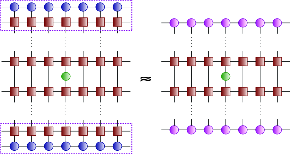
(a) Standard contraction strategy along the time direction.

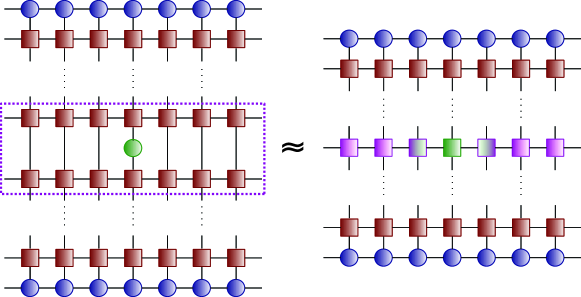
(b) Contraction in the Heisenberg picture.

Figure 3: Standard (tDMRG) and Heisenberg picture strategies to contract the tensor network

A different contraction strategy is the evolution of local operators using tDMRG in the Heisenberg picture [14, 33]. As illustrated in figure 3(b), this corresponds to contracting the problem tensor network also in the time direction, but from inside out, successively approximating the evolved operator, $\hat{O}(t)$, by a MPO. This strategy can beat the standard tDMRG approach when the evolved operators have a good approximation, or even an exact expression, as MPO, while the evolved state shows a linear increase of entanglement [34, 35], but in more general cases may require also exponential resources [36].

Other time evolution methods have been proposed based on a light cone strategy [37, 38]. They can also be understood as the contraction of an effective 2D tensor network.

\psfrag{contractL}[c][c]{contraction}\psfrag{contractR}[c][c]{}\psfrag{O}[c]{$E_{O}$}\psfrag{E}[c]{$E$}\psfrag{L}[c]{$\langle L|$}\psfrag{R}[c]{$|R\rangle$}\includegraphics[height=390.25534pt]{figure4a.eps}

(a) Transverse contraction along space direction.

\psfrag{O}[bc][bc]{$\tilde{E}_{O}$}\psfrag{E}[bc][bc]{$\tilde{E}$}\psfrag{L}[c][c]{$\langle\tilde{L}|$}\psfrag{R}[c][c]{$|\tilde{R}\rangle$}\psfrag{F}[cl][cl]{\parbox{86.72267pt}{folding axis}}\includegraphics[height=390.25534pt]{figure4b.eps}

(b) Folding of the network.

Figure 4: Contraction of the network for a local expectation value $\langle O(t)\rangle$ with the basic transverse strategy (a) and folding (b), where operators for the same time step are grouped together in a double effective operator.

Here we will focus on the transverse folding technique, introduced in [15]. Different to the approaches mentioned above, in this algorithm the tensor network is contracted along the spatial direction [see figure 4], thus avoiding the explicit truncation of the evolved state. In this scheme no TNS approximation for the state $|\Psi(t)\rangle$ is explicitly built.

Let us assume that the operator $\hat{O}$ is a single-body observable acting on site $M$.  By construction, every column in the tensor network is a MPO. For any site $k\neq M$, this MPO exactly corresponds to the transfer matrix of the evolved state [9], $E^{[k]}(t)=\sum_{i}{\bar{A}}^{[k]^{i}}(t)\otimes A^{[k]^{i}}(t)$, where $A^{[k]^{i}}(t)$ has itself a MPO structure, or more precisely, is a CTN as defined in [18]. Indeed, $A^{[k]^{i}}(t)$ is given by the local operators that act on site $k$ at all times, and represents exactly the evolved MPS. For site $M$, the MPO includes the application of the operator, $E_{O}^{[M]}(t)=\sum_{i,j}[{\bar{A}}^{[M]^{i}}(t)\otimes A^{[M]^{j}(t)}]\langle i|O|j\rangle$. In terms of the transfer matrices, the expectation value can be written

$$\langle\Psi(t)|O|\Psi(t)\rangle=\mathrm{tr}(E^{[1]}\ldots E_{O}^{[M]}\ldots E^{[N]}).$$ (2)

In the case of a finite chain, the contraction can be performed in an approximate way using the technique introduced in [26, 39]. The leftmost term, $E^{[1]}$, is a vector, with MPS structure. The product $E^{[1]}E^{[2]}$ is then read as the left action of a MPO on a MPS, which can be approximated by a MPS. Iterating this and proceeding in the same way for the right part of the network, $\langle\Psi(t)|O|\Psi(t)\rangle=\langle L_{M}|E_{O}^{[M]}|R_{M}\rangle$, where $\langle L_{M}|$ and $|R_{M}\rangle$ represent the vectors resulting from the contraction of the half-networks to the left and right of site $M$, respectively [see figure 4(a)]. If these vectors are approximated by MPS, the remaining contraction can be done exactly in an efficient way.

2.3 Transverse contraction for an infinite chain

The transverse approach is particularly convenient when dealing with an infinite chain. In this case, the resulting 2D tensor network for a given total evolution time $t$ is infinite in space, but finite in the time direction. Contraction techniques that follow the time direction typically rely on the translational invariance of the system [40, 3] for this scenario. This limits their applicability in situations that break the symmetry, as in the presence of impurities. The efficiency of the contraction in the space direction, in contrast, is not affected if the breaking of the translational symmetry occurs only for a finite sub-chain. Cases where the chain is periodic can also be treated in a similar manner.

In the thermodynamic limit, the time-dependent observable (2) will be given by

$$\langle\Psi(t)|O|\Psi(t)\rangle=\lim_{n\rightarrow\infty}\mathrm{tr}(E^{[-n+1]}\ldots E_{O}^{[M]}\ldots E^{[n-1]}).$$

If the system is translationally invariant, all columns will be identical, $E^{[k]}\equiv E(t)$, except for the one containing the application of the operator, $E_{O}$. If $\lambda$ is the eigenvalue of the transfer matrix $E$ with the largest magnitude, and it is the only one with this absolute value (the generic case for MPS [9]), $\left[E(t)\right]^{k}\sim\lambda^{k}|R\rangle\langle L|$ for large $k$. The infinite right and left half networks can thus be reduced to vectors which are proportional to the dominant right and left eigenvectors of $E(t)$, respectively $|R\rangle$ and $\langle L|$. The proportionality factors can be eliminated by normalizing,

$$\langle O(t)\rangle=\frac{\langle\Psi(t)|O|\Psi(t)\rangle}{\langle\Psi(t)|\Psi(t)\rangle}=\frac{\langle L|E_{O}|R\rangle}{\langle L|E|R\rangle}.$$ (3)

The networks that represent the numerator and denominator differ only in the single site where the operator acts, which for the latter contains the identity in the place of $\hat{O}$. If an even-odd decomposition of the Hamiltonian is used, the network is not translationally invariant, but we can recover this property blocking together pairs of sites, and the above procedure is still valid.

The dimension of the vector space on which operators $E(t)$ act grows exponentially with the number of time steps, so that in general it will not be possible to compute $|R\rangle$ and $\langle L|$ exactly. However, finite MPS tools can be used also in this case to perform the contraction in the space direction and find MPS approximations to the dominant eigenvectors. In particular, we implement the power method, by repeatedly applying the transfer matrix $E(t)$ (already written as a MPO along the time direction, see figure 4(a)) to the left and to the right of an arbitrary initial MPS vector and truncating the result to a given bond dimension, $D$, as described in [13, 39], until convergence is attained. This procedure yields a MPS approximation to the eigenvectors, with the truncation taking always place in the space of transverse vectors. The result of (3) is then obtained by computing two expectation values of MPO in states given by MPS.

If the non-degenerate dominant eigenvector of the transfer matrix $E(t)$ can be well approximated by a MPS with small bond dimension, the procedure described above will efficiently yield a good approximation to the time-dependent observable. But if the bond dimension required for the MPS approximation grows fast with time, the method will face a similar problem to the standard contraction in the time direction. Since, roughly speaking, MPS are best at describing states with small entanglement, the success of this approach will then be related to the amount of entanglement in the transverse dominant eigenvectors. We will discuss next how, in some cases, this amount can be dramatically reduced by folding.

2.4 Folding the tensor network

The folding technique combines the transverse contraction described above with a more efficient representation of the entanglement in the dominant eigenvectors. This strategy can be physically motivated by the picture of a freely propagating excitation, initially localized at one site of the chain. Although the initial state is a product, in the evolved state after time $t$, sites at a distance proportional to $2t$ become entangled. In the transverse direction this translates, after contracting from the right until a given position, $x$, into entanglement between time sites that correspond to the instant in which the excitation reaches $x$. Folding the network in two along the space-like line for the final time [see figure 1(b)] groups these sites together, and thus removes all the transverse entanglement.

On a given MPO column in figure 4(a), tensors that represent the same factor of the unitary decomposition, for the same time step in the state and its adjoint, are located at the same distance of the center of the network (corresponding to the final time, $t$). The folding transformation brings together these pairs and defines a new MPO, as shown in figure 4(b).

The folding operation can also be explained as the equivalent contraction $\langle\Psi(t)|O|\Psi(t)\rangle=\langle\Phi|O\otimes\mathbb{1}\left(|\Psi(t)\rangle\otimes|\bar{\Psi}(t)\rangle\right),$ where $|\bar{\Psi}(t)\rangle$ is the complex conjugate of $|\Psi(t)\rangle$. The bra corresponds to the product of (unnormalized) maximally entangled pairs between each site of the chain and its conjugate, $|\Phi\rangle=\left[\sum_{i_{k}=1}^{d}|i_{k}\bar{i}_{k}\rangle\right]^{\otimes N}$. We can now group together each tensor in the $|\Psi(t)\rangle$ network with the corresponding one in the adjoint, and define the effective tensors of the folded network in which the bond and physical dimensions are squared.

After folding, the network can be contracted using the transverse technique above. If the pattern of entanglement is similar to that in the intuitive picture, it will be possible to find good approximations to the dominant eigenvectors using MPS of reduced bond dimension.

3 Understanding the entanglement in the network

As evident from the discussion above, the various MPS techniques to compute time dependent expectation values will be sensitive to the amount of entanglement in the vectors or operators that each one of them needs to approximate. Here we will focus on the outside-in approaches in the time and space directions, where the partial contraction of the TN involves MPS approximations to different vectors. In the Heisenberg picture approach, the relevant quantity is the entanglement in the operator space, discussed in [34].

To better understand the different entanglement structures that can appear in the evolution network when contracted along different directions, we introduce a simple toy model, which mimics the dynamics of freely propagating excitations via a tensor network. We analyze the entanglement to which this simple model gives rise in each contraction direction. Although a true Hamiltonian dynamics generates a more complicated tensor network, this picture is useful to give us some intuition about the entanglement patterns that time-like and space-like strategies can handle efficiently. It also shows how identifying the main entanglement contribution may be the key to an efficient accurate approximation of the result of the contraction.

In the second part of the section, we make this statements more quantitative by looking at the real time evolution of a spin chain under a family of nearest-neighbour Hamiltonians. We consider in particular, a family of Hamiltonians

$$H=-\sum_{i}\left(\sigma_{z}^{i}\sigma_{z}^{i+1}+g\sigma_{x}^{i}+h\sigma_{z}^{i}\right),$$ (4)

with Ising $ZZ$ interactions and a magnetic field which may have components in the transverse, $g$, and parallel, $h$, directions. This family has two well studied limits. When $h=0$, we recover the integrable Ising model in a transverse field, critical at $g=1$, and for which the exact solution is known, whereas for $g=0$ we obtain a classical model, as the Hamiltonian is diagonal in the computational basis. Intermediate values of $g$ correspond to non-integrable models.

3.1 A tensor network toy model

We consider sites with physical dimension $d=4$. We can represent each site as composed by two two-level systems, $|a\rangle_{\ell}\otimes|b\rangle_{r}$, and identify the occupied state of the left (right) subsystem, $|1\rangle_{\ell(r)}$, with the presence in this position of a particle propagating to the left (right). The dynamics of these particles can be modelled by a simple MPO which acts as a tensor product on left- and right-moving particles, as depicted in figure 5,

$$\tilde{A}_{\tilde{\alpha}\tilde{\beta}}^{\tilde{i}\tilde{j}}\equiv\left(A_{L}\right)_{\alpha_{\ell}\beta_{\ell}}^{i_{\ell}j_{\ell}}\otimes\left(A_{R}\right)_{\alpha_{r}\beta_{r}}^{i_{r}j_{r}},$$ (5)

where $\tilde{i}\equiv i_{\ell}i_{r}$, and all the indices of tensors $A_{L}$ and $A_{R}$ have dimension two. The only non-vanishing components or the tensor are

$$\left(A_{L}\right)_{00}^{00}=\left(A_{L}\right)_{10}^{10}=\left(A_{L}\right)_{01}^{01}=\left(A_{L}\right)_{11}^{11} = 1,$$

$$\left(A_{R}\right)_{00}^{00}=\left(A_{R}\right)_{10}^{01}=\left(A_{R}\right)_{01}^{10}=\left(A_{R}\right)_{11}^{11} = 1.$$

\psfrag{L}[c][c]{$A_{L}$}\psfrag{R}[c][c]{$A_{R}$}\psfrag{a}[cl][cl]{$\alpha_{\ell}$}\psfrag{b}[cl][cl]{$\beta_{\ell}$}\psfrag{c}[cl][cl]{$i_{\ell}$}\psfrag{d}[cl][cl]{$j_{\ell}$}\psfrag{e}[cl][cl]{$\alpha_{r}$}\psfrag{f}[cl][cl]{$\beta_{r}$}\psfrag{g}[cl][cl]{$i_{r}$}\psfrag{h}[cl][cl]{$j_{r}$}\psfrag{A}[l][l]{$\equiv\tilde{A}_{\tilde{\alpha}\tilde{\beta}}^{\tilde{i}\tilde{j}}$}\includegraphics[width=195.12767pt]{figure5.eps}

Figure 5: Simple MPO that mimics the dynamics of freely propagating excitations.

This MPO is a unitary transformation which simply shifts type $\ell$ particles one site to the left, and type $r$ ones one site to the right. The graphical representation (figure 5) encompasses the actual action of the tensors, which swap the state of the physical (vertical) indices to the virtual (horizontal) ones. It is possible to easily characterize how entanglement develops in this tensor network depending on the initial state.

First we consider an initial product state in which each site is in a maximally entangled state of one particle moving to the left and one moving to the right, $\frac{1}{\sqrt{2}}\left(|1\rangle_{\ell}|0\rangle_{r}+|0\rangle_{\ell}|1\rangle_{r}\right)$. This mimics the intuitive picture of initially localized excitations that create entanglement when travelling away. Because the evolution affects left- and right-particles independently, we immediately see that after $t$ applications of the MPO the maximally entangled pairs, which were initially localized, stretch over a distance $2t$. Therefore the entanglement across any cut of the chain will grow linearly with time, and the bond dimension of the evolved state will grow exponentially.

We can easily compute the transverse dominant eigenvectors of the evolution network. The tensors acting on the transverse vectors are obtained by rotating $A_{L}$ and $A_{R}$ 90 degrees to the right, which has the effect of exchanging $L$ and $R$ terms. Taking into account that the adjoint of the MPO is also obtained by exchanging both terms, the transfer matrix will have a structure [figure 6]

$$E(t)=\langle B|\left(A_{R}\stackrel{{\scriptstyle(t)}}{{\ldots}}A_{R}A_{L}\stackrel{{\scriptstyle(t)}}{{\ldots}}A_{L}\right)\otimes\left(A_{L}\stackrel{{\scriptstyle(t)}}{{\ldots}}A_{L}A_{R}\stackrel{{\scriptstyle(t)}}{{\ldots}}A_{R}\right)|\bar{B}\rangle,$$ (6)

where $B$ is the tensor corresponding to the initial state and we have omitted the explicit left and right indices of each tensor for simplicity. The tensor product of the middle term reflects the separable evolution of the left- and right-particles. Both components can only be connected by the initial state which, in the case we are considering, is the maximally entangled state between both, so that the tensor $B$ has components $(B_{\Phi})_{i_{\ell}i_{r}}=\frac{1}{\sqrt{2}}\delta_{i_{\ell}i_{r}}$. It is easy to check that the following state is invariant under the transfer matrix, so it is an eigenvector with unit eigenvalue,

$$|R_{\Phi}\rangle=\otimes_{k=1}^{t}\left[\frac{1}{\sqrt{2}}\left(|0\rangle_{\ell_{k}}|0\rangle_{\ell_{\bar{k}}}+|1\rangle_{\ell_{k}}|1\rangle_{\ell_{\bar{k}}}\right)\otimes\frac{1}{\sqrt{2}}\left(|0\rangle_{r_{k}}|0\rangle_{r_{\bar{k}}}+|1\rangle_{r_{k}}|1\rangle_{r_{\bar{k}}}\right)\right],$$ (7)

where $|0\rangle_{\alpha_{k}}$ represents the state of the $\alpha$ ($\ell$ or $r$) subsystem at the time site corresponding to the $k-th$ application of the MPO. The subindex $\bar{k}$ refers to the symmetric time site, i.e. the $k-th$ application of the adjoint MPO.

\psfrag{k}[c][c]{$k$}\psfrag{b}[c][c]{$\bar{k}$}\includegraphics[height=650.43pt]{figure6a.eps}

\psfrag{k}[c][c]{$k$}\psfrag{l}[c][c]{$\ell_{k}$}\psfrag{r}[c][c]{$r_{k}$}\includegraphics[height=650.43pt]{figure6b.eps}

\psfrag{k}[c][c]{$k$}\psfrag{l}[c][c]{$\ell_{k}$}\psfrag{r}[c][c]{$r_{k}$}\includegraphics[height=650.43pt]{figure6c.eps}

Figure 6: Entanglement structures in the toy TN model. In (a) we show the transverse matrix $E(t=3)$ for the toy model tensor network (6); in (b) and (c) we represent the dominant right eigenvectors for this operator in the cases, respectively, of a maximally entangled and a product initial state, as described in the text.

Then, for each time step $k$, the dominant eigenvector contains a product of two maximally entangled pairs, one in the left and one in the right component of the network, stretching over a distance $2(t-k)$, which are represented in figure 6. The bond dimension required to write this vector as a MPS will then grow exponentially with time.

After folding, time sites $k$ and $\bar{k}$ are grouped in an effective site $\tilde{k}$, which will have folded $\tilde{\ell}$ and $\tilde{r}$ components. The dominant eigenvector in the folded representation can be written as

$$|R_{\Phi}\rangle=\otimes_{k=1}^{t}\left[|\Phi_{+}\rangle_{\tilde{\ell}_{k}}\otimes|\Phi_{+}\rangle_{\tilde{r}_{k}}\right],$$ (8)

where $|\Phi_{+}\rangle_{\tilde{\ell}_{k}}=\frac{1}{\sqrt{2}}\left(|0\rangle_{\ell_{k}}|0\rangle_{\ell_{\bar{k}}}+|1\rangle_{\ell_{k}}|1\rangle_{\ell_{\bar{k}}}\right)$ is a pure state of the $\ell$ component of the new effective site $\tilde{k}$, which contains exactly the two maximally entangled left-type sub-sites of $k$ and $\bar{k}$, so that the eigenvector is written as a product state.

It is also interesting to consider the opposite limit, a case in which the entanglement will not increase with time. In particular, we have considered the product state $|1\rangle_{\ell}|1\rangle_{r}$. This is an eigenstate, invariant under the evolution MPO, and contains no entanglement in space. Nevertheless, the dominant eigenvector of the transfer matrix can be checked to be of the form [see figure 6]

$$|R_{1\otimes 1}\rangle=\otimes_{k=1}^{t}\left[|1\rangle_{{\ell}_{k}}\otimes|1\rangle_{{\ell}_{\bar{k}}}\otimes\frac{1}{\sqrt{2}}\left(|0\rangle_{r_{k}}|0\rangle_{r_{\bar{k}}}+|1\rangle_{r_{k}}|1\rangle_{r_{\bar{k}}}\right)\right].$$ (9)

Therefore the transverse vector contains also nested maximally entangled pairs, in a number that grows linearly with $t$, but only half the maximum possible amount, which was attained in the case before. In a situation like this, the transverse contraction of the original network will fail, while the standard contraction is trivial. However, folding the network reduces again the dominant eigenvector to a product, thus allowing the transverse contraction. The initial product $|0\rangle_{\ell}|0\rangle_{r}$, which could be understood as having no excitation in the system, behaves in an analogous way.

3.2 Entropy in the transverse contraction for Ising-like Hamiltonians

To make our statements more quantitative, we have compared the behaviour of entanglement in the transverse contractions, with and without folding, for time evolution under the family of Hamiltonians defined in (4). As a figure of merit we compute the maximum entanglement entropy, $S_{\mathrm{max}}$, with respect to all possible bipartitions, in the dominant right eigenvectors  at different times, and we compare this quantity before and after the folding for different Hamiltonians and initial states. Although the truncation error of the dominant eigenvectors would properly evaluate the accuracy of the transverse approaches, this entropy has a more physical interpretation. It is the analogue to the entanglement in the time direction, and allows us to connect our observations to the intuitive models.

In particular, we have studied three representative scenarios. First, we simulate a sudden quench in the integrable Ising model, starting from an initial product state, for which the entropy in the standard picture is known to grow linearly with time. Second, we take the opposite limit, and set the initial state to be the ground state of the evolving Hamiltonian. Naively, these two scenarios correspond to the cases described for the toy model in the previous section. Finally, we consider a more general quench, in which the initial state is the entangled ground state of (4) for certain values of $g$, $h$, and evolves under a different set of parameters, not corresponding to any integrable limit.

Figure 7 shows the results corresponding to the first of these cases, when the chain is initialized in a product state, $|X+>\equiv\left[\frac{1}{\sqrt{2}}(|0\rangle+|1\rangle)\right]^{\otimes N}$, in which all spins are aligned along the positive $\hat{x}$ direction, and evolves under the Ising Hamiltonian (4) with fixed transverse field $g=1.1$ (and $h=0$). In this limit, the Hamiltonian is equivalent to a free fermion model, and the initial state $|X+\rangle$ corresponds to the fermionic Fourier vacuum [41], containing a superposition of all products of pairs of diagonal modes with opposite momenta $k$ and $-k$. Therefore, one may expect that this scenario shows the closest similarity to the intuitive picture of freely propagating excitations described in section 2.4. Actually, the entropy in the evolved state is known to grow linearly with time. In our toy model such a situation led to linearly growing entanglement in the transverse contraction, which could be completely removed by folding. From the numerical results we observe that the entropy in the transverse eigenvector grows indeed linearly with time (the apparent saturation obeys to truncation in the eigenvector at a given bond dimension $D$, an effect shown explicitly in figure 8), and the maximal entropy of the folded eigenvector, while having a value different from zero, saturates very fast, in agreement with the intuitive expectation, and remains constant at longer times. The actual asymptotic value of $S_{max}^{\mathrm{(folded)}}$ and the slope of $S_{max}^{\mathrm{(unfolded)}}$ depend on the particular parameter $g$. As $g$ decreases, the latter grows slower, until for $g=0$, the classical model is recovered and both values coincide.

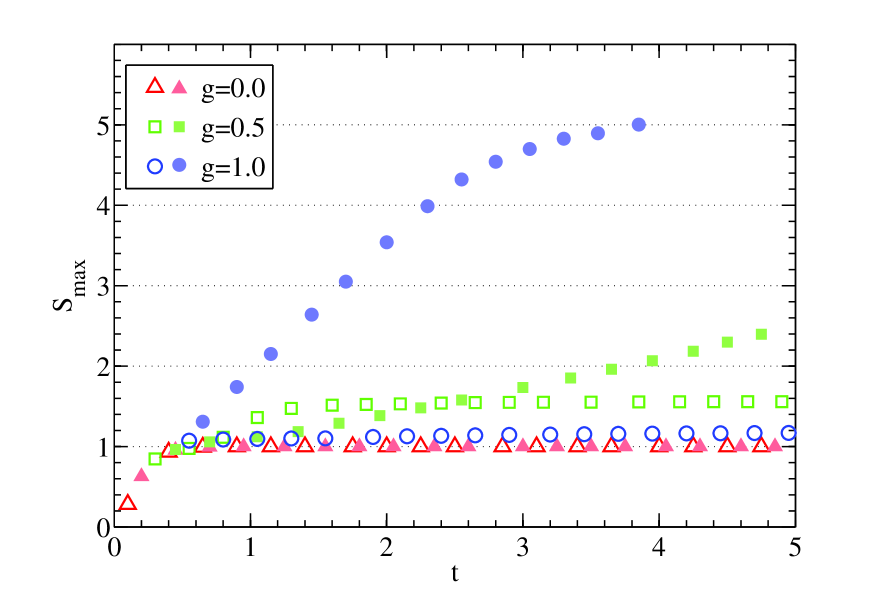
Figure 7: Maximal entropy in the transverse dominant eigenvectors as a function of time in the evolution of a product state $|X+\rangle$ under the exactly solvable Ising model (vanishing parallel field $h=0$) with transverse field $g=1$ (blue circles), $0.5$ (green squares) and $0$ (red triangles). The solid symbols correspond to the original network and the empty ones to the folded case.

These observations corroborate the simplified picture for out-of-equilibrium situations in which we can expect excitations propagating in the state and creating correlations at long distances as time evolves. In those scenarios, the growing correlation length makes it difficult for a standard MPS approach to describe the evolved state, and we thus expect the maximum gain from folding the tensor network.

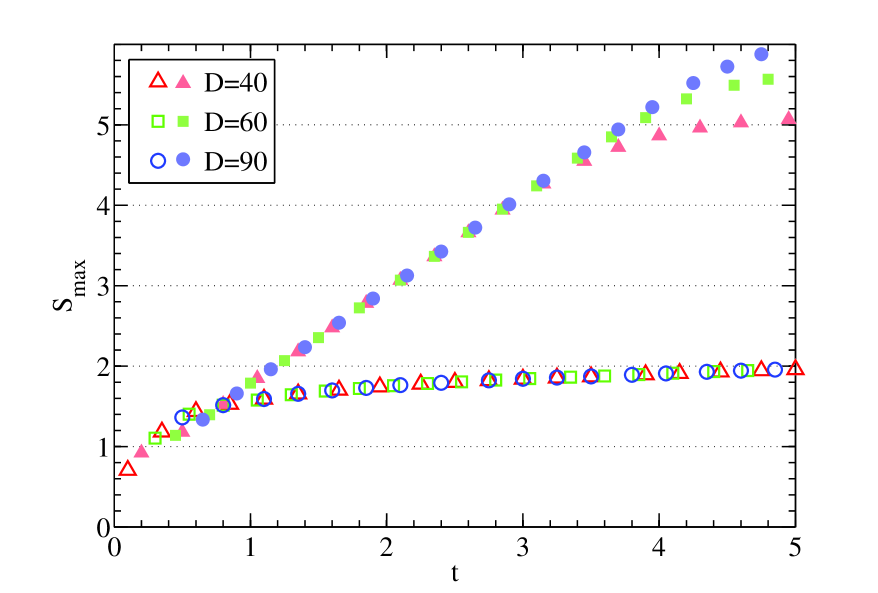
Figure 8: Maximal entropy in the transverse dominant eigenvectors as a function of time in the integrable Ising model with $g=1.1$, $h=0$, for initial ground state. The solid (empty) symbols correspond to the original (folded) network, using bond dimension $D=40$ (red triangles), $60$ (green squares) and $90$ (blue circles) for the eigenvector. As apparent from the curves for the original network, a fixed $D$ can keep track of the linear increase in entropy only for a certain time, after which truncation is evident.

The opposite situation would be that of an eigenstate of the Hamiltonian, which along the evolution will only acquire a time-dependent phase. If the state was well described by an MPS, as will often be the case for the ground state, it will still be a MPS at any later time, but the transverse picture may introduce entanglement in the contraction, as for the invariant state under the toy model in section 3.1. We have thus looked at the entropy in the transverse eigenvectors, both with and without folding, starting from an MPS approximation to the ground state of the integrable Ising model ($g=1.1$, $h=0$). The initial MPS approximation was found via the iTEBD algorithm [3] with bond dimension $\chi=8$, to an accuracy in energy of the order or $10^{-7}$. The entropy results are shown in figure 8. We observe good agreement with the intuitive understanding from section 3.1, with entropy growing linearly in the transverse contraction before folding, whereas after folding it grows very slowly for long times, appearing almost saturated.

Finally, we want to explore the entropy properties of a more general case, which does not correspond to the toy model described above. To this end, we consider a more general dynamics ($h\neq 0$) where the free fermion picture does not apply, and we simulate a global quench in which we start from the ground state for $g=1.1$, $h=0$, as above, and evolve the system under various Hamiltonians, with fixed $g$ and varying $h$.

The results are shown in figure 9. We observe that for small $h$, the behaviour is close to that in figure 8, most favourable for the folding strategy. As the parallel component of the magnetic field $h$ grows, the difference between entropies before and after folding seems to decrease, and at some point, the maximum entropy is smaller before the folding. Even in these cases, the folded entropy lies well below the upper bound $2S_{\mathrm{max}}^{\mathrm{(unfolded)}}$, which would be reached if there was no entanglement between the pairs of tensors the folding brings together. A more determinant property than the absolute value of $S_{\mathrm{max}}$ at a certain moment, at least concerning the utility of these algorithms, is its scaling with time, as this will ultimately determine the length of the evolution we can simulate with these techniques. Remarkably, for the case $h\simeq g$ we observe that both curves have a similar pattern, with the entropy saturating or growing very slowly for long times. This seems to indicate that in this case, both techniques would support long time calculations.

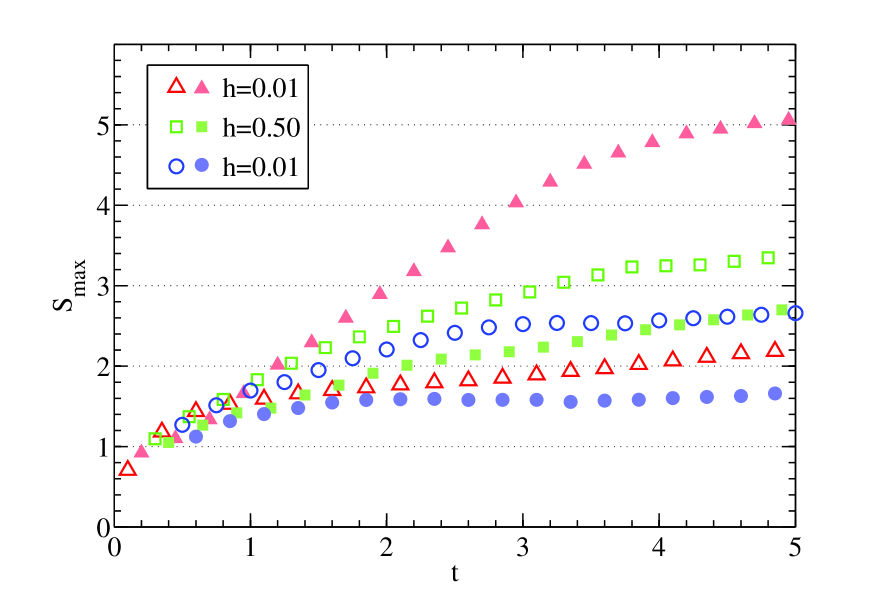
Figure 9: Maximal entropy in the transverse dominant eigenvectors as a function of time, after a quench of the parallel field $h$. The system starts in the ground state of (4) with $g=1.1$, $h=0$ and evolves under a different Hamiltonian with fixed transverse $g=1.1$ and varying parallel field $h=0.01$ (red triangles), $0.5$ (green squares) and $1$ (blue circles). Solid (empty) symbols correspond to the original (folded) network.

4 Applications and results

In this section, we describe several physical problems in which the transverse and folding techniques can be useful. We adapt the techniques to the various scenarios and illustrate these applications with the results for two families of spin models.

On one hand, we consider the Ising model, as defined in (4). To complete our analysis, we present results also for simulations of the XY model,

$$H_{XY}=-\sum_{i}\left(J_{x}\sigma_{x}^{i}\sigma_{x}^{i+1}+J_{y}\sigma_{y}^{i}\sigma_{y}^{i+1}+J_{z}\sigma_{z}^{i}\right),$$ (10)

equivalent to a free-fermion case, too, and thus expected to show similar features to our simplistic model.

In the following, we will exclusively consider chains in the thermodynamic limit. Although the basic techniques of folding and transverse contraction can be applied both to infinite and finite networks, the main advantage of using the folding strategy is due to the entanglement structure of the dominant eigenvectors that reduce the infinite network to a finite contraction. In a finite case, on the contrary, the 2D network to be contracted spans the whole range of spatial sites, and in general the entanglement content of the transverse vectors will be complicated due to the boundary effects.

4.1 Out of equilibrium evolution

A particularly interesting problem for these transverse strategies is given by the out-of-equilibrium evolution of an infinite chain after a global quench. This kind of dynamics can create fast growing entanglement between spatial sites. According to our intuitive model and the entropy analysis discussed in the previous sections, the transverse folding strategy should be best suited for this scenario, being most advantageous when the scaling of the spatial entanglement with time is the largest possible.

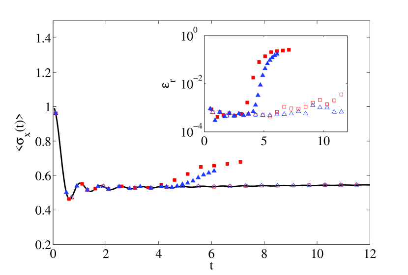
Figure 10: Transverse magnetization per site $\langle\sigma_{x}(t)\rangle$ as a function of time for the evolution under the Ising model with $g=1.05$ of the initial product state $|X+\rangle$. The solid line is the exact result, and the solid (empty) symbols show the results obtained with the transverse (folded) contraction using bond dimension $D=60$ (red squares) and $120$ (blue triangles) for the eigenvectors. The inset shows the relative error.

Following from the study of the transverse entropies in the last section, a good realization of this intuitive picture occurs in the evolution, under the exactly solvable Ising model, of an initial product state $|X+\rangle$. In this situation, the Hamiltonian is equivalent to a free-fermion model, and the entanglement in the space direction is known to grow linearly with time. This scenario was already discussed in [15], where we computed the time dependent local magnetization as a function of time (shown in figure 10), and checked the adequacy of the folding transverse contraction to compute time-dependent local observables.

Another instance of a free-fermion model is the XY chain of (10). In [42] the entanglement entropy of a block was analytically computed and it was shown that, as for the Ising model, it can grow linearly with time after a global quench. It is then interesting to check how accurately this scenario connects to the free-propagating picture. We have therefore explored the transverse entanglement in this model for what should be the closest scenario to the ideal case of freely propagating excitations, i.e. the evolution of the Fourier fermionic vacuum. The initial state corresponds now to the product of all spins aligned along the negative $\hat{z}$ direction, $|Z-\rangle\equiv\left[|1\rangle\right]^{\otimes N}$. Figure 11 shows the compared maximal entropies for transverse and transverse-folded dominant right eigenvectors in this case. Qualitatively, the difference in scaling reproduces the situation for the analogous Ising case depicted in figure 7, with a dramatic change of slope for the folded case which leads to a very slow increase at long times. This change, however, occurs at a later time, and for larger absolute values of entropy in the case of the XY chain than for the Ising model. Therefore, even if the transverse folded eigenvectors can be well approximated by MPS of bound dimension at long times, the largest difference with respect to the transverse contraction without folding is likely to be evident only at much longer times. The XY Hamiltonian, however, does not admit such an efficient decomposition of the evolution operator as in the case of the Ising model [16]. Even for the lowest Trotter order, the XY evolution requires at least twice as many MPO per step as in the Ising case, what increases the computational cost of the simulations in an equivalent factor.

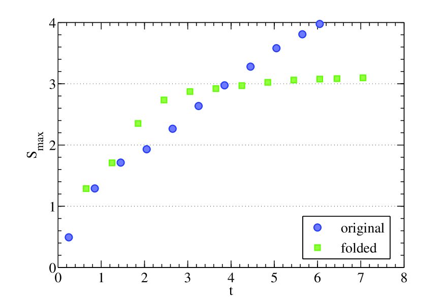
Figure 11: Maximal entropy in the transverse dominant eigenvectors as a function of time in the evolution of the product state $|Z-\rangle$ under the exactly solvable XY model (10) with parameters $J_{x}=1.5$, $J_{y}=0.5$ and $J_{z}=0$. The simulations were run using a first order Trotter expansion and maximum bond dimension $D=90$ for the dominant right eigenvectors in the original network (green triangles) and the folded one (blue circles).

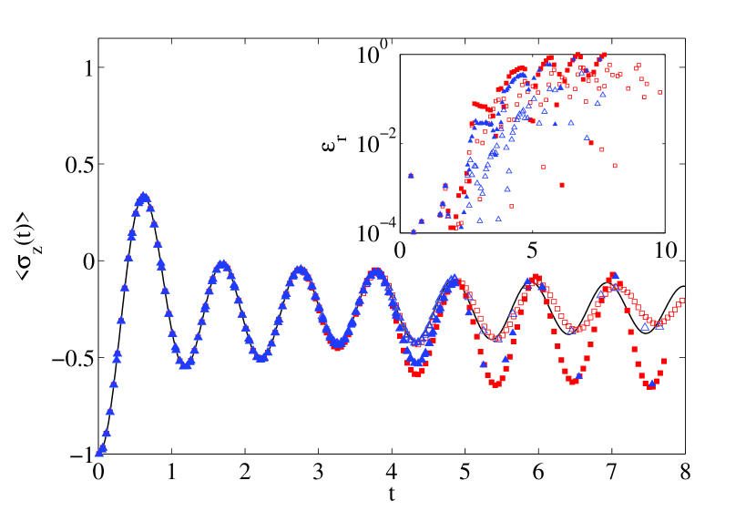
Figure 12: Magnetization per site $\langle\sigma_{z}(t)\rangle$ as a function of time for the evolution, under the XY model with $J_{x}=-1$, $J_{y}=0.5$, $J_{z}=0$, of the initial product state $|Z-\rangle$. The solid line is the exact result, and the solid (empty) symbols show the results obtained with the transverse (folded) contraction using bond dimension $D=60$ (red squares) and $90$ (blue triangles) for the eigenvectors. The inset shows the relative error.

Figure 12 shows the results for the time-dependent polarization per site, $\langle\sigma_{z}(t)\rangle$, when evolving the product state $|Z-\rangle$ under the XY Hamiltonian. The folded strategy with bond dimension $D=90$ attains an accuracy of the order of $10^{-2}$ at times $t\simeq 6$, which compares positively to results obtained with a light-cone based method for a similar model in [37].  Moreover, we can observe the different behaviour of errors before and after folding. The unfolded contraction deviates clearly from the exact curve after $t\simeq 4$ and increasing the bond dimension from $D=60$ to $90$ does not significantly improve the error. The folded version, instead, seems to oscillate around the proper mean value, albeit somehow slower. Increasing the bond dimension from $D=60$ to $90$ in this case has the effect of bringing the oscillations closer to the exact pattern, corroborating the smoother onset of errors which was already detected in [15].

4.2 Dynamical correlators

Often, specially relevant observables are given by another kind of dynamical quantities, namely time-dependent two-point correlation functions, $\langle O_{2}^{[i_{2}]}(t_{2})O_{1}^{[i_{1}]}(t_{1})\rangle$, computed in the ground state of the system, and it is then desirable that the numerical methods are able to evaluate them.

\psfrag{A}[l][l]{$t_{2}-t_{1}$}\psfrag{B}[l][l]{$t_{1}$}\psfrag{C}[bc][bc]{$i_{1}$}\psfrag{D}[bc][bc]{$i_{2}$}\includegraphics[height=390.25534pt]{figure13a.eps}

(a) 2D network representing the two-point correlator $C_{12}(i_{1}\ t_{1},i_{2}\ t_{2})$ in the general case.

\psfrag{C}[c]{$i_{1}$}\psfrag{D}[c]{$i_{2}$}\psfrag{A}[c][c]{$\langle L|$}\psfrag{B}[c][c]{$|R\rangle$}\includegraphics[height=390.25534pt]{figure13b.eps}

(b) Transverse contraction reduces to a finite network.

Figure 13: Scheme of the tensor network for the two-point time dependent correlator $\langle O_{2}^{[i_{2}]}(t_{2})O_{1}^{[i_{1}]}(t_{1})\rangle$ for $i_{2}>i_{1}$ and $t_{2}>t_{1}$.

Even if the ground state possesses translational invariance, an expectation value of this type breaks it, and any contraction technique in the time direction will see its efficiency reduced, as it will have to keep track of the causal cone of different tensors spreading from the application of the first operator. The transverse techniques, on the other hand, can be easily adapted to compute these observables with the same cost as correlators at equal times.

Let us consider times $t_{2}>t_{1}$, and distance $\Delta=i_{2}-i_{1}>0$. The two-body correlator computed in a general (not necessarily the fundamental) state $|\Psi\rangle$ can be written as

$$C_{12}^{(\Psi)}(i_{1}\ t_{1},i_{2}\ t_{2}) \equiv \langle\Psi|O_{2}^{[i_{2}]}(t_{2})O_{1}^{[i_{1}]}(t_{1})|\Psi\rangle$$

$$= \langle\Psi|U(t_{2},0)^{\dagger}O_{2}^{[i_{2}]}U(t_{2},t_{1})O_{1}^{[i_{1}]}U(t_{1},0)|\Psi\rangle,$$

where $U(t_{2},t_{1})$ is the evolution operator from time $t_{1}$ to $t_{2}$. If the state $|\Psi\rangle$ is expressed as a MPS, we can again represent this quantity by a tensor network, by approximating each of the evolution operators in this expression as a product of MPO terms [figure 13(a)]. The infinite part of the network is the same as in the case of a single body observable acting at time $t_{2}$, and can then be reduced to the left and right dominant eigenvectors of the transfer matrix,

$$C_{12}(i_{1}\ t_{1},i_{2}\ t_{2})=\frac{\langle L|E_{O_{2}(t_{2})}E^{\Delta-1}E_{O_{1}(t_{1})}|R\rangle}{\langle L|E^{\Delta+1}|R\rangle},$$ (11)

where now $E=E(t_{2})$ is the transfer matrix resulting from evolution until the longest time $t_{2}$, and $E_{O_{i}(t_{i})}$ is the column MPO operator corresponding to site $i$, on which a single-body operator acts at time $t_{i}$ [see figure 13(b)]. The cost of finding the dominant eigenvectors is determined by the time $t_{2}$, as in the case of a single-body expectation value. The width of the finite network left to be contracted after this step is $\Delta+3$. In particular, if both operators act on the same site, the computation has the same cost as that of $\langle O_{2}(t_{2})\rangle$.

It is also possible to apply the folding method to the TN in 13(a). From the toy model and the entropy results in figure 8, we expect that for the dynamical correlators computed in the ground state the folded eigenvectors have a more efficient description in terms of MPS and produce better approximations.

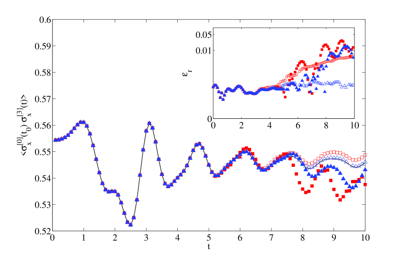
Figure 14: Two-spin dynamical correlator $\langle\sigma_{x}^{[i]}(t_{0})\sigma_{x}^{[i+\Delta]}(t_{0}+t)\rangle$ as a function of time, in the ground state of the Ising model ($g=1.1$, $h=0$), at distance $\Delta=3$ using $t_{0}=0.1$. Shown are the exact result (solid line) and the results from the transverse (solid symbols) and folded transverse (empty symbols) contractions, using bond dimension $D=60$ (red squares) and $90$ (blue triangles), and a fourth order Trotter expansion with $\delta=0.1$. The inset shows the relative error for each series of data. The approximation to the ground state, with an accuracy in energy of $10^{-7}$, was computed with iTEBD, using bond dimension $\xi=16$.

To apply the transverse techniques to these quantities, we need to express also the state in which the correlator is to be computed, in this case the ground state of the model, as a tensor network.

We could find an appropriate TN description of the ground state by combining real and time evolution steps in the same TN, so that the first part of the evolution is in imaginary time, and produces a TN approximation to the ground state and the second part, in real time, approximates the dynamics. Here we proceed with a simpler alternative, which consists in first finding a MPS approximation to the ground state by means of the iTEBD method, and then using the obtained tensor as the initial state in our dynamical TN.

We have checked the algorithm with the computation of the two-spin correlation function $\langle\sigma_{x}^{[i]}(t_{0})\sigma_{x}^{[i+\Delta]}(t_{0}+t)\rangle$ in the ground state of the Ising model with $g=1.1$, using the transverse and folding strategies and comparing them to the exact values. Our results, in figure 14, show that the folding strategy achieves better accuracy for the same bond dimension, $D=90$, and is able to reach a relative error $\epsilon_{r}\approx 10^{-4}$ at times $t\approx 10$. We also observe again the smoother appearance of errors in the folded algorithm.

\psfrag{D}[l][l]{$t_{2}-t_{1}$}\psfrag{e}[r][l]{}\includegraphics[width=173.44534pt]{figure15.eps}

Figure 15: Minimal TN for the calculation of dynamical two-point correlators in the ground state, to which the network in figure 13(a) is reduced if the MPS initial state is the ground state of the evolving Hamiltonian.

The combined use of iTEBD and the transverse technique provides us with another, yet more efficient way of computing the dynamical correlators (11) in the ground state. Indeed, if $|\Psi\rangle=|\phi_{0}\rangle$ is the ground state of the Hamiltonian, with energy $E_{0}$, the correlator can be simplified, $C_{12}^{(\phi)}(i_{1}\ t_{1},i_{2}\ t_{2})=e^{i(t_{2}-t_{1})E_{0}}\langle\Psi|O_{2}^{[i_{2}]}e^{-i(t_{2}-t_{1})H}O_{1}^{[i_{1}]}|\Psi\rangle$. The contraction in this expression admits a simpler TN description than the general case (see figure 15), which again can be efficiently contracted in the transverse direction.

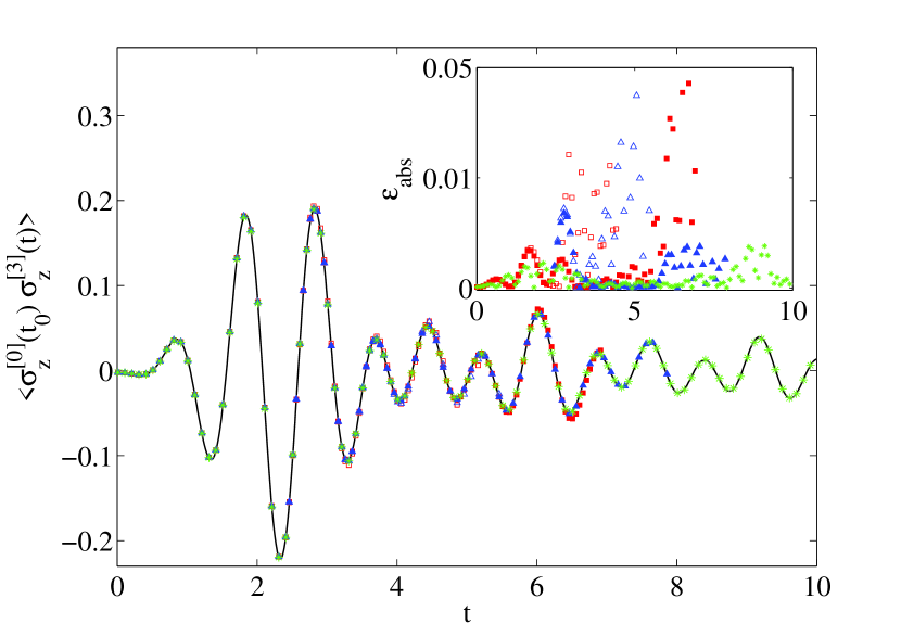
Figure 16: Two-spin correlator $\langle\sigma_{z}^{[i]}(t_{0})\sigma_{z}^{[i+\Delta]}(t_{0}+t)\rangle$ as a function of time, in the ground state of the XY model with $J_{x}=1.5$, $J_{y}=0.5$, $J_{z}=0$), at distance $\Delta=3$ using $t_{0}=0.01$. Shown are the exact result (solid line) and the results from the transverse (solid symbols) and folded transverse (empty symbols) contractions, using bond dimension $D=60$ (red squares) and $90$ (blue triangles), and a first order Trotter expansion with $\delta=0.01$. The green stars show the results for the minimal TN transverse contraction with $D=60$. The inset shows the absolute error for each series. The iTEBD approximation to the ground state was obtained, using bond dimension $\xi=8$, with an accuracy in energy of $10^{-6}$.

We have checked the performance of this description and compared it to the other transverse strategies in the case of the XY model. The results, in figure 16, show the clear advantage of the minimal TN contraction, which achieves good agreement with the exact values to times $t\approx 10$ with bond dimension as small as $D=60$. The transverse and folded contraction of the original network were performed with bond dimensions up to $D=90$. At the times simulated, the contraction without folding achieves better results than after folding. These relatively short times simulated are however not enough to conclude whether that will still be the case at longer times. The entropy scaling, shown in figure 17, suggests the opposite.

We can compare the maximal entropy $S_{max}$ in the dominant eigenvectors for each of the three methods (figure 17). Qualitatively, the behaviour of the transverse and folded strategies agrees with the previous observations for the ground state in the Ising case (figure 8), with seemingly linear increase in the case of the original TN and a much slower growth in the case of the folded network for long times. The maximal entropy for the minimal TN is much lower and also grows slower than the others, in agreement to the much better results achieved with this technique.

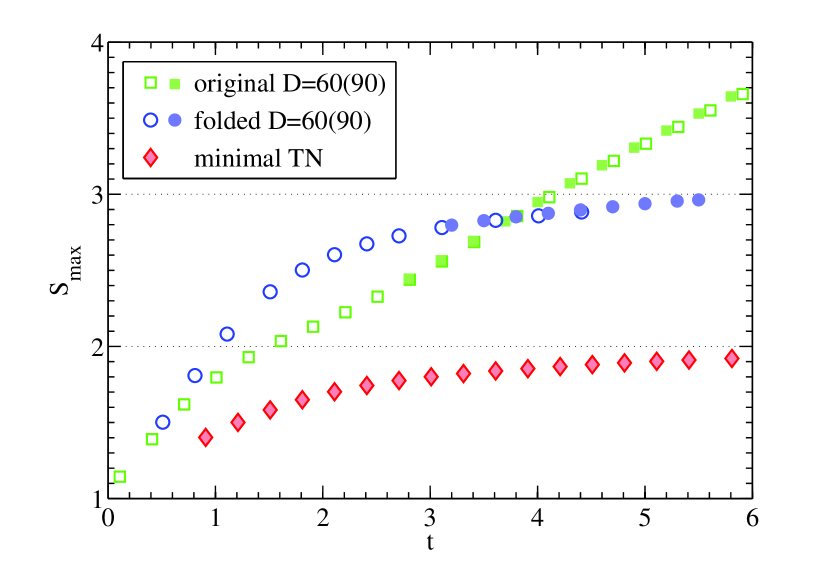
Figure 17: Maximal entropy as a function of time for the transverse dominant eigenvectors in the tensor networks that describe the dynamical correlators in the XY model with $J_{x}=1.5$, $J_{y}=0.5$ and $J_{z}=0$. The ground state approximation was a MPS with bond dimension $\xi=8$. Shown are the results for the original transverse network (green squares), the folded network (blue circles) and the minimal TN (red diamonds).

4.3 Imaginary time evolution

The basic technique described in Sect. 2.1 to approximate the action of an evolution operator as a composition of locally acting MPO can also be used for a real exponential. Therefore the same methods can be used to simulate imaginary time evolution of infinite chains and to compute their ground state properties. Since the ground state is the limit

$$|\Psi_{0}\rangle=\lim_{\tau\rightarrow\infty}\frac{e^{-H\tau}|\Phi_{0}\rangle}{\|e^{-H\tau}|\Phi_{0}\rangle\|},$$

we may compute the expectation value of any observable in the ground state as

$$\langle O\rangle_{\Psi_{0}}\approx\frac{\langle\Phi_{0}|e^{-H\tau}Oe^{-H\tau}|\Phi_{0}\rangle}{\langle\Phi_{0}|e^{-2H\tau}|\Phi_{0}\rangle}$$ (12)

in the limit of large $\tau$. This quantity can be also estimated by contracting a two dimensional tensor network, obtained in this case from the application of small steps of imaginary time evolution, $e^{-H\delta}$, approximated in terms of non-unitary MPO factors. The structure of the resulting network is similar, with the transfer matrix replaced by an operator whose left and right dominant eigenvectors, if not degenerate, are enough to reduce the network to a finite one. Notice that in this case, the maximum eigenvalue of the transfer matrix does not need to be one. It is possible to use the same techniques described before to find a MPS approximation to the dominant eigenvectors and compute the observables. The transverse operators appearing in this problem are closely related to those in the transfer matrix DMRG approach [23, 24].

Although the equilibrium properties of local Hamiltonians are typically well described by the standard approach, i.e. by approximating the ground (or thermal) state by a MPS, there are cases in which the transverse strategy can be advantageous. This will be particularly true in the thermodynamic limit, in any situation that breaks the translational invariance.

Here we describe how the transverse (folded) tensor network can be adapted to describe two types of equilibrium observables which can benefit from this alternative, namely the ground state properties in the presence of impurities and the computation of thermal properties.

4.3.1 Ground states of non-translationally invariant problems (impurities)

The problem of finding the ground state of an infinite spin chain with one or more impurities breaks the translational invariance and thus poses a problem for a time-like contraction method, like iTEBD, which will need to keep track of an increasing number of tensors (the causal cone generated by the impurity) along the imaginary time evolution. On the contrary, the transverse picture can deal with the problem with similar computational cost as in the purely translationally invariant case.

As a test case, we considered a modification of the Ising chain in a transverse field $H=-\left(\sum_{i}\sigma_{z}^{i}\sigma_{z}^{i+1}+g_{i}\sigma_{x}^{i}\right)$, with the magnetic impurity at position $i=0$, i.e. the magnetic field is constant over the chain, $g_{i}\equiv g$ $\forall i\neq 0$, except at the origin, where it takes the value $g_{0}$. This case was already analyzed in [15], and we only summarize here the results for completeness.

The tensor network that represents the ground state obtained by imaginary time evolution will be very similar to the translationally invariant one obtained for uniform magnetic field. Since the impurity affects only a localized term in the Hamiltonian, only the column operators neighbouring $i=0$ will change.  In particular, the computation of the left and right dominant eigenvectors will not be affected by the impurity, which will only appear in the final contraction of the finite tensor network. The particular network to be contracted will depend then on the observable we want to calculate. Figure 18 pictures the resulting tensor network for the computation of the site dependent magnetization, $\langle\sigma_{x}^{[i]}\rangle$, i.e. the magnetization at distance $i$ from the impurity. The numerical results, in figure 19, illustrate the success of the algorithm at describing the screening of the impurity for different values of the magnetic field at the origin.

\psfrag{i0}[c]{$i=0$}\psfrag{ix}[c]{$i=x$}\psfrag{langle}{$\langle L|$}\psfrag{rangle}{$|R\rangle$}\includegraphics[width=173.44534pt]{figure18.eps}

Figure 18: Scheme of the tensor network for the magnetization at a distance $x$ of the magnetic impurity. The leftmost operator (green) represents the only column which is affected by the presence of the impurity.

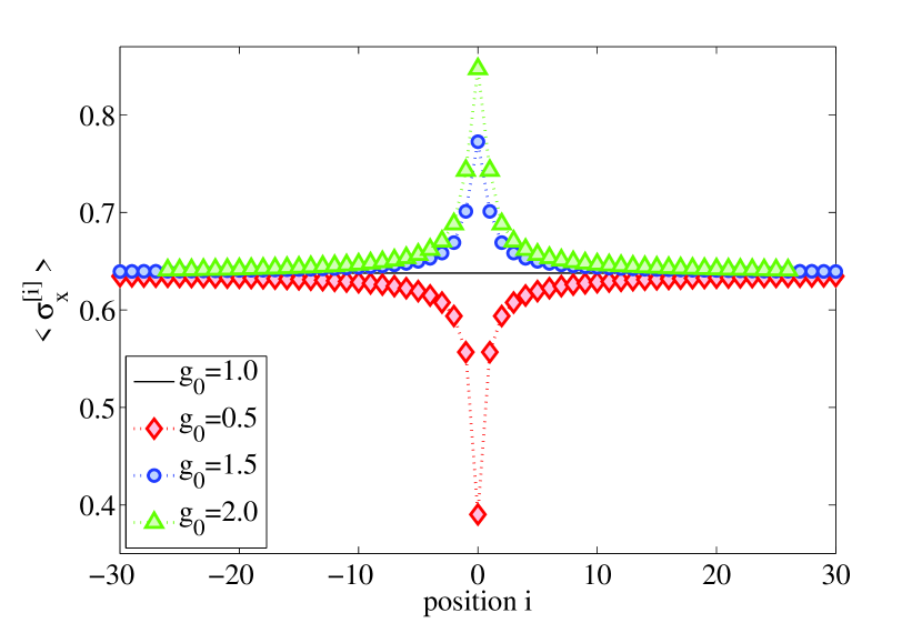
Figure 19: Ground state magnetization as a function of the distance to the localized impurity in the Ising chain, for $g=1$ on every site except at the origin, where $g_{0}=0.5$ (red diamonds), $1.5$ (blue circles) and $2$ (green triangles). The solid line shows the magnetization in the uniform case ($g_{0}=1$). The results were obtained using bond dimension $D=40$ for the transverse eigenvectors, without folding the network, with imaginary time evolution long enough for convergence ($10^{-6}$ in the energy) of the critical Ising ground state.

4.3.2 Thermal states

The transverse folded network can be modified to represent the thermal equilibrium state of a local Hamiltonian. Although it is possible to efficiently approximate such thermal state by a MPO [44], and there are efficient algorithms to find this kind of description [13], it is worth mentioning that the standard approach already proceeds in a folded space, as it must work with MPO and not MPS. Therefore folding the network does not increase the effective dimension of the sites with respect to the standard direction of contraction. Additionally, since the folding contraction does not construct the MPO description of the state, it can avoid some difficulties the standard method needs to face, such as imposing positivity of the density matrix. Moreover, the transverse approach can be specially useful when the translational invariance is broken, as could be in the localized impurity problem. Finally, imaginary and real time evolutions can also be combined to compute time dependent observables from the thermal state, such as dynamical correlators at finite temperature.

The thermal density matrix at inverse temperature $\beta$, for the Hamiltonian $H$, up to normalization, is given by the exponential $\rho_{th}(\beta)\propto\mathrm{e}^{-\beta H}=\mathrm{e}^{-\frac{\beta}{2}H}\mathbb{1}\mathrm{e}^{-\frac{\beta}{2}H}$. This is formally identical to the evolution of the identity operator in imaginary time ${\beta}/{2}$ under the Hamiltonian $H$. The exponential operators in this expression can be also approximated by the same Trotter expansion described in section 2.1, so that the density matrix can be expressed as a two dimensional tensor network, as shown in figure 20(a). To compute the expectation value of a given local observable we need to evaluate the trace $\mathrm{tr}[\hat{O}\rho_{th}(\beta)]$. To this end, we apply the operator $O$ and sum over all indices which, in the pictorial representation of the tensor network, corresponds to connecting pairs of open legs. The result [see figure 20(b)] is a naturally folded network, where the folding axis is taken to lie along the initial identity operator. This network is very similar to the one obtained after folding for the imaginary time evolution of a pure state, differing only in the tensors that occupy the place of the initial state. In fact, the thermal network is equivalent to the asymmetric contraction $\langle\Phi|(\hat{O}\mathrm{e}^{-\frac{\beta}{2}H}\otimes\mathrm{e}^{-\frac{\beta}{2}\bar{H}})|\Phi\rangle$. The network can be thus contracted using the transverse method in a completely analogous manner to the imaginary time evolution of a pure state after folding, and the remaining norm factor can be computed in the same way for the identity operator $\hat{O}=\mathbb{1}$.

\psfrag{contractL}[c][c]{contraction}\psfrag{contractR}[c][c]{}\psfrag{identity}[bc][bc]{$\mathbb{1}$}\psfrag{step}[bc][bc]{$\mathrm{e}^{-\delta\beta H}$}\includegraphics[height=390.25534pt]{figure20a.eps}

(a) 2D network representing the unnormalized thermal state $\rho(\beta)$.

\psfrag{op}[c][c]{$O$}\psfrag{tra}[c][c]{\parbox{130.08731pt}{traced indices}}\psfrag{langle}[c][c]{$\langle\tilde{L}|$}\psfrag{rangle}[c][c]{$|\tilde{R}\rangle$}\psfrag{fol}[cl][cl]{\parbox{86.72267pt}{folding axis}}\includegraphics[height=390.25534pt]{figure20b.eps}

(b) Transverse contraction of the network for a thermal expectation value.

Figure 20: Expectation values in thermal states correspond naturally to a folded network.

We checked the accuracy of thermal expectation values computed with this method using the exactly solvable Ising model as a benchmark. As shown in the figures, very accurate results are obtained with a modest bond dimension. A relative error in the energy below $\varepsilon=10^{-5}$ is achieved for bond dimension $D=20$ (figure 21). In figure 22 we show also the good convergence of the spin-spin correlations with a bond dimension of only $D=10$ for the transverse eigenvectors.

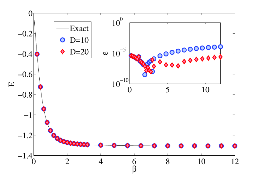
Figure 21: Energy per particle as a function of the inverse temperature $\beta$ in the thermal state for the integrable Ising model with $g=1.05$. The plot shows the exact result (solid line) and the energy computed with the folding method for bond dimension 10 (blue circles) and 20 (red stars), using a fourth order Trotter expansion with step $\delta=0.1$. The inset shows the relative error.

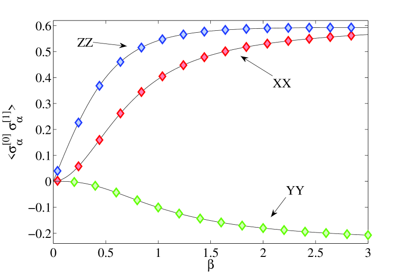
Figure 22: Nearest-neighbour correlations in the thermal state as a function of the inverse temperature $\beta$ in the thermal state for the integrable Ising model with $g=1.05$. The plot shows the exact result (solid line) for three types of spin-spin correlations, and the numerical results (diamonds) obtained with the folding method for bond dimension 10, using a fourth order Trotter expansion with step $\delta=0.1$.

5 Discussion

In this work we have analyzed in some depth the properties of the transverse folding method, recently introduced for the dynamical simulation of infinite quantum spin chains. The folding method restates the problem of computing time dependent observables as a two dimensional tensor network contraction, in which the second dimension corresponds to time. Some of the previously existing algorithms for simulating time evolution can also be reinterpreted as different strategies for the contraction of this network. The performance of the various methods is then related to the entanglement structures that appear in the network, depending on its boundaries, which include the initial state, and on the direction chosen to perform the contraction.

We have presented a dynamical model defined by a tensor network that, despite its simplicity, exhibits the main characteristics of the contraction that depend on the direction and the initial state. In particular, the scaling of entanglement with time can be very different depending on the contraction strategy, thus deciding the success or failure of one approach or another. Notably, some of the extreme cases in which one technique overpowers the other can be easily understood from the features of the toy model.

We have also studied the reduction of transverse entanglement achieved by folding in the case of a real Hamiltonian evolution, under a family of models of the Ising type. We have found that the folding strategy often results in a more favourable scaling of the entanglement with time, even in some cases that are far from the ideal picture of free-propagating excitations that motivates this approach.

We can conclude that, although in most problems the time extent that can be simulated by these methods will remain limited, understanding the entanglement contents in the state and also in the time direction can be determinant to decide on the feasibility of a given simulation, and to choose the most convenient simulation method for a particular scenario.

As we have discussed, transverse contraction strategies, including the folding of the TN, can be applied to a variety of physical problems involving infinite chains. In particular, to situations that break translational invariance, as can be the presence of impurities, and to the computation of two-body correlations at different times.

References

- [1] G. Vidal. Efficient classical simulation of slightly entangled quantum computations. Phys. Rev. Lett., 91(14):147902, 2003.
- [2] A. J. Daley, C. Kollath, U. Schollwöck, and G. Vidal. Time-dependent density-matrix renormalization-group using adaptive effective hilbert spaces. J. Stat. Mech., 2004(04):P04005, 2004.
- [3] G. Vidal. Classical simulation of infinite-size quantum lattice systems in one spatial dimension. Phys. Rev. Lett., 98:070201, 2007.
- [4] I. Affleck, T. Kennedy, E. H. Lieb, and H. Tasaki. Valence bond ground states in isotropic quantum antiferromagnets. Commun. Math. Phys., 115:477, 1988.
- [5] A. Klumper, A. Schadschneider, and J. Zittartz. Equivalence and solution of anisotropic spin-1 models and generalized t-j fermion models in one dimension. J. Phys. A, 24(16):L955–L959, 1991.
- [6] A. Klumper, A. Schadschneider, and J. Zittartz. Groundstate properties of a generalized vbs-model. Z. Phys. B, 87:281, 1992.
- [7] M. Fannes, B. Nachtergaele, and R. F. Werner. Finitely correlated states on quantum spin chains. Commun. Math. Phys., 144:443–490, 1992.
- [8] F. Verstraete, D. Porras, and J. I. Cirac. Density matrix renormalization group and periodic boundary conditions: A quantum information perspective. Phys. Rev. Lett., 93:227205, 2004.
- [9] D. Perez-García, F. Verstraete, M. M. Wolf, and J. I. Cirac. Matrix product state representations. Quantum Inf. Comput., 7:401, 2007.
- [10] P. Calabrese and J. Cardy. Evolution of entanglement entropy in one-dimensional systems. J. Stat. Mech., 2005(04):P04010, 2005.
- [11] N. Schuch, M. M. Wolf, F. Verstraete, and J. I. Cirac. Entropy scaling and simulability by matrix product states. Phys. Rev. Lett., 100(3):030504, 2008.
- [12] T. Osborne. Efficient approximation of the dynamics of one-dimensional quantum spin systems. Phys. Rev. Lett., 97:157202, 2006.
- [13] F. Verstraete, J. J. García-Ripoll, and J. I. Cirac. Matrix product density operators: Simulation of finite-temperature and dissipative systems. Phys. Rev. Lett., 93(20):207204, 2004.
- [14] S R Clark, J Prior, M J Hartmann, D Jaksch, and M B Plenio. Exact matrix product solutions in the heisenberg picture of an open quantum spin chain. New Journal of Physics, 12(2):025005, 2010.
- [15] Mari-Carmen Bañuls, Matthew B. Hastings, Frank Verstraete, and J. Ignacio Cirac. Matrix product states for dynamical simulation of infinite chains. Phys. Rev. Lett., 102:240603, 2009.
- [16] B. Pirvu, V. Murg, J. I. Cirac, and F. Verstraete. Matrix product operator representations. New Journal of Physics, 12(2):025012, 2010.
- [17] H. F. Trotter. On the product of semi-groups of operators. Proc. Amer. Math. Soc., 10(4):545–551, 1959.
- [18] R. Hübener, V. Nebendahl, and W. Dür. Concatenated tensor network states. New Journal of Physics, 12(2):025004, 2010.
- [19] M. Suzuki. Fractal decomposition of exponential operators with applications to many-body theories and monte carlo simulations. Phys. Lett. A, 146(6):319–323, 1990.
- [20] M. Suzuki. General theory of fractal path integrals with applications to many-body theories and statistical physics. J. Math. Phys., 32(2):400–407, 1991.
- [21] M. Suzuki. General decomposition theoory of ordered exponentials. Proc. Japan Acad., 69(B):161–166, 1993.
- [22] Norbert Schuch, Michael M. Wolf, Frank Verstraete, and J. Ignacio Cirac. Computational complexity of projected entangled pair states. Phys. Rev. Lett., 98:140506, Apr 2007.
- [23] R. J. Bursill, T. Xiang, and G. A. Gehring. The density matrix renormalization group for a quantum spin chain at non-zero temperature. J. Phys. Condens. Matter, 8(40):L583–L590, 1996.
- [24] X. Wang and T. Xiang. Transfer-matrix density-matrix renormalization-group theory for thermodynamics of one-dimensional quantum systems. Phys. Rev. B, 56(9):5061–5064, Sep 1997.
- [25] Tomotoshi Nishino and Kouichi Okunishi. Corner transfer matrix renormalization group method. Journal of the Physical Society of Japan, 65(4):891–894, 1996.
- [26] F. Verstraete and J. I. Cirac, 2004.
- [27] H. H. Zhao, Z. Y. Xie, Q. N. Chen, Z. C. Wei, J. W. Cai, and T. Xiang. Renormalization of tensor-network states. Phys. Rev. B, 81:174411, May 2010.
- [28] Ling Wang, Iztok Pižorn, and Frank Verstraete. Monte carlo simulation with tensor network states. Phys. Rev. B, 83:134421, Apr 2011.
- [29] Román Orús and Guifré Vidal. Simulation of two-dimensional quantum systems on an infinite lattice revisited: Corner transfer matrix for tensor contraction. Phys. Rev. B, 80:094403, Sep 2009.
- [30] A. García-Saez and J. I. Latorre. Renormalization group contraction of tensor networks in three dimensions. arXiv:1112.1412v1 [cond-mat.str-el], 2011.
- [31] Steven R. White and Adrian E. Feiguin. Real-time evolution using the density matrix renormalization group. Phys. Rev. Lett., 93(7):076401, Aug 2004.
- [32] U. Schollwöck and S. White. Methods for time dependence in dmrg. In G. G. Batrouni and D. Poilblanc, editors, Effective Models for Low-Dimensional Strongly Correlated Systems, volume 816 of American Institute of Physics Conference Series, pages 155–185, 2006.
- [33] Dominik Muth, Razmik G. Unanyan, and Michael Fleischhauer. Dynamical simulation of integrable and nonintegrable models in the heisenberg picture. Phys. Rev. Lett., 106:077202, Feb 2011.
- [34] Toma ž Prosen and Iztok Pižorn. Operator space entanglement entropy in a transverse ising chain. Phys. Rev. A, 76:032316, Sep 2007.
- [35] Iztok Pižorn and Toma ž Prosen. Operator space entanglement entropy in spin chains. Phys. Rev. B, 79:184416, May 2009.
- [36] Toma ž Prosen and Marko Žnidarič. Is the efficiency of classical simulations of quantum dynamics related to integrability? Phys. Rev. E, 75:015202, Jan 2007.
- [37] M. B. Hastings. Observations outside the light-cone: Algorithms for nonequilibrium and thermal states. Phys. Rev. B, 77:144302, 2008.
- [38] Tilman Enss and Jesko Sirker. Light cone renormalization and quantum quenches in one-dimensional hubbard models. New Journal of Physics, 14(2):023008, 2012.
- [39] V. Murg, F. Verstraete, and J. I. Cirac. Variational study of hard-core bosons in a two-dimensional optical lattice using projected entangled pair states. Phys. Rev. A, 75(3):033605, 2007.
- [40] Stellan Östlund and Stefan Rommer. Thermodynamic limit of density matrix renormalization. Phys. Rev. Lett., 75(19):3537–3540, Nov 1995.
- [41] Subir Sachdev. Quantum phase transitions. Cambridge University Press, 1999.
- [42] Maurizio Fagotti and Pasquale Calabrese. Evolution of entanglement entropy following a quantum quench: Analytic results for the chain in a transverse magnetic field. Phys. Rev. A, 78:010306, Jul 2008.
- [43] F. Naef, X. Wang, X. Zotos, and W. von der Linden. Autocorrelations from the transfer-matrix density-matrix renormalization-group method. Phys. Rev. B, 60(1):359–368, Jul 1999.
- [44] M. B. Hastings. Solving gapped hamiltonians locally. Phys. Rev. B, 73:085115, Feb 2006.