The generalized Krawtchouk polynomials and the fifth Painlevé equation

Abstract

We study the recurrence coefficients of the orthogonal polynomials with respect to a semi-classical extension of the Krawtchouk weight. We derive a coupled discrete system for these coefficients and show that they satisfy the fifth Painlevé equation when viewed as functions of one of the parameters in the weight.

2010 MSC: 34M55, 33E17, 33C47, 42C05, 65Q30

Keywords: discrete orthogonal polynomials; semi-classical extension of the Krawtchouk weight; recurrence coefficients; Painlevé equations

1 Introduction

1.1 Orthogonal polynomials

It is well-known (see, for instance, [4, 19]) that a sequence of orthonormal polynomials $(p_{n})_{n\in\mathbb{N}}$, i.e.,

$$\int p_{m}(x)p_{n}(x)\,d\mu(x)=\delta_{m,n},$$ (1.1)

where $\mu$ is a positive measure with support on the real line and $\delta_{m,n}$ is the Kronecker delta, satisfies a three-term recurrence relation

$$xp_{n}(x)=a_{n+1}p_{n+1}(x)+b_{n}p_{n}(x)+a_{n}p_{n-1}(x)$$ (1.2)

with the recurrence coefficients given by the following integrals

$$a_{n}=\int xp_{n}(x)p_{n-1}(x)\,d\mu(x),\qquad b_{n}=\int xp_{n}^{2}(x)\,d\mu(x).$$ (1.3)

Here it is assumed that $p_{-1}=0$.

We will consider discrete orthogonal polynomials for which the weight is supported on an equidistant lattice $\{hn+n_{0}|\,n\in A\subset\mathbb{Z}\}$ with parameters $h$ and $n_{0}$. In case of the lattice $\mathbb{N}_{0}=\{0,1,\ldots\}$ the orthogonality condition (1.1) reads

$$\sum_{k=0}^{\infty}p_{m}(k)p_{n}(k)\,w(k)=\delta_{m,n}.$$ (1.4)

The examples of (classical) discrete orthogonal polynomials on an equidistant lattice include the Meixner and Charlier polynomials with the lattice $\mathbb{N}_{0}$ and the Krawtchouk and Hahn polynomials ($N+1$ polynomials orthogonal on $\{0,1,$ $\ldots,$ $N\}$). For more information about discrete (classical) orthogonal polynomials, we refer to [19, 26] (see also [2, 9, 10] for the definitions of classical weights and their semi-classical extensions and further references).

A useful characterization of classical polynomials is the Pearson equation

$$[\sigma(x)w(x)]^{\prime}=\tau(x)w(x),$$

where $\sigma$ and $\tau$ are polynomials satisfying $\deg\sigma\leq 2$ and $\deg\tau=1$. In case of discrete polynomials on a linear lattice the Pearson equation reads

$$\nabla[\sigma(x)w(x)]=\tau(x)w(x),$$

where $\nabla$ is the backward difference operator

$$\nabla f(x)=f(x)-f(x-1).$$

Semi-classical orthogonal polynomials are defined as orthogonal polynomials for which the weight satisfies a Pearson equation for which $\deg\sigma>2$ or $\deg\tau\neq 1$ (see [18, 23]). The recurrence coefficients in the three-term recurrence relation (1.2) for classical orthogonal polynomials (e.g., Hermite, Laguerre, Jacobi, Charlier, Meixner, Krawtchouk and others) can be found explicitly in contrast to non-classical weights. The recurrence coefficients of semi-classical weights usually obey nonlinear recurrence relations, which, in many cases, can be identified as discrete Painlevé equations; see for instance [3, 22] and the references therein. Moreover, when viewed as functions of one of the parameters in the weight, the recurrence coefficients satisfy (continuous) Painlevé equations (see [2, 9, 10] in case of the discrete semi-classical Meixner and Charlier weights and [11] and the references therein for other semi-classical continuous weights). This paper gives another example of the connection between discrete orthogonal polynomials and the Painlevé equations.

1.2 Statement of the results

The classical Krawtchouk polynomials for each $N\in\mathbb{N}$ and $n\leq N$ are defined by

$$K_{n}(x)={}_{2}F_{1}\left(-n,-x;-N;\frac{1}{p}\right),\quad p\in(0,1),$$ (1.5)

where

$${}_{2}F_{1}\left(a,b;c;z\right)=\sum_{s=0}^{\infty}\frac{(a)_{s}(b)_{s}}{(c)_{s}s!}z^{s},$$

with the Pochhammer symbol $(a)_{n}$ being defined by

$$(a)_{n}=\prod_{j=0}^{n-1}(a+j)=a(a+1)\cdots(a+n-1),$$

is the hypergeometric function; cf. [8, Chapter 15]. They satisfy orthogonality conditions with respect to the binomial weight

$$w(k)=\binom{N}{k}p^{k}(1-p)^{N-k},\quad k\in\{0,1,\ldots,N\}.$$

The polynomials satisfy (1.2) for $n=0,\ldots,N-1$ with $K_{-1}=0$ and $a_{0}=0$. The Krawtchouk polynomials are, in fact, the Meixner polynomials

$$M_{n}(x)={}_{2}F_{1}\left(-n,-x;\beta;1-\frac{1}{\ell}\right)$$

with $\beta=-N$ and $\ell=p/(p-1)$. The recurrence coefficients for the orthonormal Krawtchouk polynomials are given by

$$a_{n}^{2}=np(1-p)(N+1-n),\quad b_{n}=p(N-n)+n(1-p).$$ (1.6)

Observe that $a_{0}^{2}=0=a_{N+1}^{2}$.

In this paper, we are concerned with a semi-classical generalization of Krawtchouk polynomials with the weight function defined by

$$w(x)=\binom{N}{x}\frac{c^{x}}{(1-\alpha)_{x}},\qquad x\in\{0,\ldots,N\},$$ (1.7)

where $\alpha<1$ and $c>0$ are two real parameters. Note that we can recover the Krawtchouk weight from (1.7) by letting $c$ and $-\alpha$ tend to infinity and $-\frac{c}{\alpha}\to\frac{p}{1-p}$. Our first result gives a discrete system satisfied by the recurrence coefficients.

Theorem 1.1.

Let $a_{n}$ and $b_{n}$ be the recurrence coefficients in (1.2) for the weight (1.7). We then have that

$$x_{n} =\frac{1}{N}\left(\frac{a_{n}^{2}}{c}+n\right),$$ (1.8)

$$y_{n} =-\frac{b_{n}+N+1+c-n-\alpha}{N},$$ (1.9)

satisfy the following discrete system

$$\begin{cases}(x_{n}+y_{n})(x_{n+1}+y_{n})=\displaystyle-\frac{y_{n}(N+1+Ny_{n})(N+1-\alpha+Ny_{n})}{cN},\\ \\ (x_{n}+y_{n})(x_{n}+y_{n-1})=\displaystyle\frac{x_{n}(-N-1+Nx_{n})(\alpha-N-1+Nx_{n})}{N(Nx_{n}-n)},\end{cases}$$ (1.10)

with initial conditions

$$x_{0}=0,\quad y_{0}=-\frac{N+1+c-\alpha}{N}-\frac{c}{1-\alpha}\frac{M(-N+1,2-\alpha,-c)}{M(-N,1-\alpha,-c)},$$ (1.11)

where $M(a,b,z)$ is the confluent hypergeometric function ${}_{1}F_{1}(a;b;z)$ defined by

$${}_{1}F_{1}(a;b;z)=\sum_{s=0}^{\infty}\frac{(a)_{s}}{(b)_{s}s!}z^{s};$$

(cf. [8, Chapter 13]).

Recall that a truncated confluent hypergeometric function is a Laguerre polynomial, in particular $M(-N,1-\alpha,-c)=\frac{N!}{(1-\alpha)_{N}}L_{N}^{(-\alpha)}(-c)$; see [8, Eq. 13.6.19]. Hence the initial value $y_{0}$ is in terms of a ratio of Laguerre polynomials.

The system (1.10) can be obtained by a limiting procedure from $\alpha$-dP${}_{\textup{I}V}$ [15, 32] given by

$$\begin{cases}(X_{n}+Y_{n})(X_{n+1}+Y_{n})=\displaystyle\frac{(Y_{n}-\widetilde{A})(Y_{n}-\widetilde{B})(Y_{n}-\widetilde{C})(Y_{n}-\widetilde{D})}{(Y_{n}+\Gamma-Z_{n})(Y_{n}-\Gamma-Z_{n})},\\ \\ (X_{n}+Y_{n})(X_{n}+Y_{n-1})=\displaystyle\frac{(X_{n}+\widetilde{A})(X_{n}+\widetilde{B})(X_{n}+\widetilde{C})(X_{n}+\widetilde{D})}{(X_{n}+\Delta-Z_{n+1/2})(X_{n}-\Delta-Z_{n+1/2})},\end{cases}$$ (1.12)

with $\widetilde{A}+\widetilde{B}+\widetilde{C}+\widetilde{D}=0$. Indeed, by taking

$$X_{n}=x_{n}-1/\varepsilon,\quad Y_{n}=y_{n}+1/\varepsilon,$$

$$\widetilde{A}=1/\varepsilon,\quad\widetilde{B}=-3/\varepsilon+(2N+2-\alpha)/N,$$

$$\widetilde{C}=1/\varepsilon-(N+1)/N,\quad\widetilde{D}=1/\varepsilon-(N+1-\alpha)/N,$$

$$Z_{n}=(2n-1)/(2N)+1/\varepsilon,\quad\Gamma^{2}=4c/(N\varepsilon),\quad\Delta=2/\varepsilon,$$

and letting $\varepsilon$ tend to zero, we get (1.10).

It is worthwhile to point out that if we take $\alpha=0$ and $c=\frac{p}{1-p}$, the weight function (1.7) reduces to the one considered in [1], where the author derived a discrete system for the recurrence coefficients. We also observe that the system in [31], which was also used in [10] for the generalized Meixner weight, can be obtained from (1.10) with an appropriate choice of the parameters and scaling of $x_{n}$ and $y_{n}$.

Since there are two parameters in the weight (1.7), the recurrence coefficients are dependent on these parameters as well. Our next theorem shows that, when viewed as a function of $c$, the recurrence coefficients $a_{n}(c)$ and $b_{n}(c)$ are related to the fifth Painlevé equation.

Theorem 1.2.

With $x_{n}(c)$ and $y_{n}(c)$ defined in (1.8) and (1.9), we have

$$x_{n}(c)=\frac{(cy^{\prime}+n-N)^{2}-2(n-N)(n-N+cy^{\prime})y-A_{1}y^{4}+A_{2}y^{3}-A_{3}y^{2}}{4cN(y-1)y^{2}},$$ (1.13)

$$y_{n}(c)=\frac{N-n+y(1+n+c-\alpha+(\alpha-N-1)y)-cy^{\prime}}{2N(y-1)y},$$ (1.14)

where

$$A_{1}=(1+N-\alpha)^{2},\;\;A_{2}=2(1+N-\alpha)(1+c+N-\alpha),\;\;A_{3}=(1+c+n-\alpha)(1+c-n+2N-\alpha)$$

and $y=y(c)$ is the solution of the fifth Painlevé equation P${}_{\textup{V}}$

$$y^{\prime\prime}=\left(\displaystyle\frac{1}{2y}+\displaystyle\frac{1}{y-1}\right)(y^{\prime})^{2}-\displaystyle\frac{y^{\prime}}{c}+\displaystyle\frac{(y-1)^{2}}{c^{2}}\left(Ay+\displaystyle\frac{B}{y}\right)+\displaystyle\frac{Cy}{c}+\,\,\displaystyle\frac{Dy(y+1)}{y-1},$$ (1.15)

with the parameters given by

$$A=\frac{(\alpha-N-1)^{2}}{2},\;\;B=-\frac{(n-N)^{2}}{2},\;\;C=-(n+\alpha),\;\;D=-\frac{1}{2}.$$ (1.16)

Theorem 1.2 gives the relationship between $x_{n},\,y_{n}$ (and hence $a_{n}^{2},\;b_{n}$) and solutions of P${}_{\textup{V}}$  explicitly.

The Painlevé equations possess the so-called Painlevé property: the solutions have no movable branch points. They were discovered by Painlevé and his colleagues at the beginning of the twentieth century while classifying all second-order ordinary differential equations of the form

$$w^{\prime\prime}=\mathcal{R}(z,w,w^{\prime}),$$ (1.17)

where ${}^{\prime}=d/dz$, the function $\mathcal{R}$ is rational in $w$ and $w^{\prime}$, meromorphic in $z$, which possess the Painlevé property. It turns out that, up to Möbius transformations, only fifty equations of the form (1.17) have the Painlevé property [13, 29, 30]. Forty-four of these equations can either be linearized, be transformed to a Riccati equation or be solved in terms of elliptic functions. The six remaining equations are now known as the Painlevé equations, which are often referred to as nonlinear special functions [6] and have numerous applications in mathematics and mathematical physics.

The Painlevé equations cannot be solved in terms of elementary functions or known classical special functions in general. For certain combinations of parameters, however, P${}_{\textup{II}}$–P${}_{\textup{VI}}$ have solutions expressed in terms of special functions. For P${}_{\textup{V}}$, the choice of parameters (1.16) is exactly when P${}_{\textup{V}}$ admits classical solutions expressible in terms of confluent hypergeometric functions (equivalently, Kummer functions or Whittaker functions), see [8, $\S$ 32.10 (v)]. In fact, it is the case when confluent hypergeometric functions have the associated Laguerre polynomials as special cases. Hence, the condition (1.16) on the parameters in P${}_{\textup{V}}$ is actually that when P${}_{\textup{V}}$ has rational solutions (see [8, $\S$ 32.8 (v)]). This is also consistent with the initial condition (1.11) for $y_{0}$. For more information about classical and rational solutions about P${}_{\textup{V}}$ and the associated $\tau$-functions, we refer to [5, 6, 12, 16, 17, 21, 24, 25, 27, 28, 33].

The rest of this paper is devoted to the proofs of Theorems 1.1 and 1.2. They are given in Sections 2 and 3, respectively. In Section 4 we study recurrence coefficients numerically. We conclude this paper with a discussion in Section 5.

2 Proof of Theorem 1.1

The proof of Theorem 1.1 relies on the ladder operators for discrete orthogonal polynomials, which were studied in [20]. We start with a brief description of this aspect.

2.1 Ladder operators for discrete orthogonal polynomials

Given a weight function $w$, we define a potential

$$u(x)=-\frac{\nabla w(x)}{w(x)}=\frac{w(x-1)-w(x)}{w(x)},$$ (2.1)

which is a discrete analogue of the external field generated by $w$. The action of the forward difference operator

$$\Delta f(x)=f(x+1)-f(x)$$

on orthogonal polynomials $p_{n}$ is given by

$$\Delta p_{n}(x)=A_{n}(x)p_{n-1}(x)-B_{n}(x)p_{n}(x).$$ (2.2)

In case of a weight $w$ on the lattice $\mathbb{N}_{0}$ with $w(-1)=0$, the coefficients $A_{n}(x)$ and $B_{n}(x)$ in (2.2) are given by

$$A_{n}(x)=a_{n}\sum_{k\in\mathbb{N}_{0}}p_{n}(k)p_{n}(k-1)\frac{u(x+1)-u(k)}{x+1-k}w(k),$$ (2.3)

and

$$B_{n}(x)=a_{n}\sum_{k\in\mathbb{N}_{0}}p_{n}(k)p_{n-1}(k-1)\frac{u(x+1)-u(k)}{x+1-k}w(k).$$ (2.4)

In the case of a weight $w$ supported on a finite lattice $\{0,1,\ldots,N\}$ with boundary conditions $w(-1)=0$ and $w(N+1)=0$, the coefficients $A_{n}(x)$ and $B_{n}(x)$ in (2.2) are given by

$$A_{n}(x)=a_{n}\frac{p_{n}(N+1)p_{n}(N)}{N-x}w(N)+a_{n}\sum_{k=0}^{N}p_{n}(k)p_{n}(k-1)\frac{u(x+1)-u(k)}{x+1-k}w(k),$$ (2.5)

and

$$B_{n}(x)=a_{n}\frac{p_{n}(N+1)p_{n-1}(N)}{N-x}w(N)+a_{n}\sum_{k=0}^{N}p_{n}(k)p_{n-1}(k-1)\frac{u(x+1)-u(k)}{x+1-k}w(k).$$ (2.6)

In both cases, when the lattices are finite or infinite, the following compatibility relations between the functions $A_{n}$ and $B_{n}$ hold:

$$B_{n}(x)+B_{n+1}(x)=\frac{x-b_{n}}{a_{n}}A_{n}(x)-u(x+1)+\sum_{j=0}^{n}\frac{A_{j}(x)}{a_{j}},$$ (2.7)

$$a_{n+1}A_{n+1}(x)-a_{n}^{2}\frac{A_{n-1}(x)}{a_{n-1}}=(x-b_{n})B_{n+1}(x)-(x+1-b_{n})B_{n}(x)+1.$$ (2.8)

2.2 Proof of Theorem 1.1

To prove Theorem 1.1, we follow the theme in [1], which made use of the compatibility relations between the ladder operators.

It is readily seen that, with $w$ defined in (1.7), $w(-1)=0$ and $w(N+1)=0$. By (2.1), we have

$$u(x)=-1+\frac{x(x-\alpha)}{c(N+1-x)}.$$ (2.9)

It then follows from (2.5) and (2.6) that

$$A_{n}(x)=a_{n}R_{n}\frac{x}{N-x}+a_{n}T_{n}\frac{1}{N-x},$$

where

$$R_{n}=\frac{1}{c}\sum_{k=0}^{N}p_{n}(k)p_{n}(k-1)w(k),$$

$$T_{n}=p_{n}(N+1)p_{n}(N)w(N)+\frac{1}{c}\sum_{k=0}^{N}p_{n}(k)p_{n}(k-1)\frac{Nk+(N+1)(1-\alpha)}{N-k+1}w(k),$$

and

$$B_{n}(x)=\frac{x}{N-x}r_{n}+\frac{1}{N-x}t_{n}$$

with $t_{0}=0$ and

$$r_{n}=\frac{a_{n}}{c}\sum_{k=0}^{N}p_{n}(k)p_{n-1}(k-1)w(k),$$

$$t_{n}=a_{n}p_{n}(N+1)p_{n-1}(N)w(N)+\frac{a_{n}}{c}\sum_{k=0}^{N}p_{n}(k)p_{n-1}(k-1)\frac{Nk+(N+1)(1-\alpha)}{N+1-k}w(k).$$

Using the orthonormality of the polynomials one immediately gets that

$$R_{n}=\frac{1}{c},\qquad r_{n}=0,$$

since $p_{n}(k-1)=p_{n}(k)+$lower order terms. Thus, we obtain

$$A_{n}(x)=a_{n}\frac{x}{c(N-x)}+a_{n}T_{n}\frac{1}{N-x},$$

$$B_{n}(x)=\frac{t_{n}}{N-x},$$

with $t_{0}=0.$

Next we use the compatibility relations (2.7) and (2.8). The first compatibility relation (2.7) gives rise to the following two equations, after collecting coefficients of equal powers of $x$:

$$c(t_{n}+t_{n+1}+b_{n}T_{n})=-1+\alpha+cN+c\sum_{j=0}^{n}T_{j},$$ (2.10)

$$cT_{n}-b_{n}-1+\alpha-c+n=0.$$ (2.11)

From the second compatibility relation we get

$$a_{n+1}^{2}T_{n+1}-a_{n}^{2}T_{n-1}=-b_{n}t_{n+1}+(b_{n}-1)t_{n}+N,$$ (2.12)

$$a_{n+1}^{2}-a_{n}^{2}=c(t_{n+1}-t_{n}-1).$$ (2.13)

From (2.13) we find, using telescopic summation, that

$$a_{n}^{2}=c(t_{n}-n).$$ (2.14)

Equation (2.11) gives

$$b_{n}=-1-c+n+\alpha+cT_{n}.$$ (2.15)

After multiplying (2.12) by $T_{n}$ we can replace $-b_{n}T_{n}$ using (2.10), which allows us to take a telescopic sum. As a result we get

$$c^{2}(t_{n}-n)T_{n}T_{n-1}=ct_{n}^{2}+cN\sum_{j=0}^{n-1}T_{j}-ct_{n}\sum_{j=0}^{n-1}T_{j}-t_{n}(cN-1+\alpha).$$ (2.16)

One can also replace $a_{n}^{2}$ and $a_{n+1}^{2}$ in equation (2.12) using (2.14) and rewrite the obtained equation by collecting the coefficients of $t_{n+1}$ and $t_{n}$. Taking a telescopic sum and using (2.15) gives

$$c(t_{n}-n)(T_{n}+T_{n-1})+t_{n}(\alpha+n-c-2)=nN-c\sum_{j=0}^{n-1}T_{j}.$$ (2.17)

Multiplying (2.17) by $T_{n}$, using (2.16) on the left-hand side and (2.10) on the right-hand side and eliminating the sum using (2.10) we finally obtain

$$(N+cT_{n})(1-\alpha-cN+ct_{n+1}+cT_{n}(\alpha-c-2+cT_{n}))\\ +ct_{n}(N-t_{n+1}+cT_{n})=0.$$ (2.18)

Replacing the sum in equation (2.17) with the aid of (2.16) we get

$$t_{n}(1-2n+(2n-2+\alpha)(N+1)+c(n+N)T_{n}+c(n+N+cT_{n})T_{n-1})\\ =n(N+cT_{n-1})(N+cT_{n})+t_{n}^{2}(n-2+\alpha+c(T_{n}+T_{n-1})).$$ (2.19)

Setting

$$x_{n}=\frac{t_{n}}{N},\quad y_{n}=-\frac{cT_{n}}{N}-1$$ (2.20)

in the last two equations, we obtain the system (1.10).

Finally, we note that the initial conditions for the recurrence coefficients, in terms of the moments $\mu_{1}$ and $\mu_{0}$, are given by $a_{0}^{2}=0$ and

$$b_{0}=\frac{\mu_{1}}{\mu_{0}}=\frac{cN}{(1-\alpha)}\frac{M(-N+1,2-\alpha,-c)}{M(-N,1-\alpha,-c)},$$

where $M(a,b,z)$ is the confluent hypergeometric function ${}_{1}F_{1}(a;b;z)$. This, together with (1.8) and (1.9), implies initial conditions (1.11) for $x_{n}$ and $y_{n}$.

This completes the proof of Theorem 1.1.

3 Proof of Theorem 1.2

We use the method proposed in [2, 10] and system (1.10) to prove Theorem 1.2. We repeat the main steps to be self-contained.

To prove the theorem, we derive the differential equation for $y_{n}$. In [2, 10] we have used the Toda system

$$\begin{cases}\displaystyle\left(a_{n}^{2}\right)^{\prime}:=\frac{d}{dc}\left(a_{n}^{2}\right)=\frac{a_{n}^{2}}{c}(b_{n}-b_{n-1}),\\ \displaystyle b_{n}^{\prime}:=\frac{d}{dc}b_{n}=\frac{1}{c}(a_{n+1}^{2}-a_{n}^{2}),\end{cases}$$ (3.1)

which also holds in the present case. Solving the first equation (1.10) for $x_{n+1}$ and the second equation for $y_{n-1}$ and substituting into the Toda system (3.1) (where we have replaced $a_{n}^{2}$ and $b_{n}$ by their expressions in terms of $x_{n}$ and $y_{n}$ from Theorem 1.1), we get two equations

$$x_{n}^{\prime} = \frac{Nx_{n}-n}{c}\left(-x_{n}-y_{n}+\frac{x_{n}(-N-1+Nx_{n})(\alpha-N-1+Nx_{n})}{N(Nx_{n}-n)(x_{n}+y_{n})}\right)$$

and

$$y_{n}^{\prime} = x_{n}+y_{n}+\frac{y_{n}(N+1+Ny_{n})(N+1-\alpha+Ny_{n})}{cN(x_{n}+y_{n})},$$ (3.2)

where the differentiation is with respect to $c$. By differentiating equation (3.2) and substituting the expression for $x_{n}^{\prime}$ we obtain an equation for $y_{n}^{\prime\prime}$ as a function of $y_{n}^{\prime},y_{n},x_{n}$:

$$y_{n}^{\prime\prime} = -\frac{1}{c}(Nx_{n}-n)(x_{n}+y_{n})+\frac{x_{n}(-N-1+Nx_{n})(\alpha-N-1+Nx_{n})}{cN(x_{n}+y_{n})}+y_{n}^{\prime}$$

$$+ \frac{y_{n}^{\prime}}{Nc(x_{n}+y_{n})}\left((N+1+Ny_{n})(N+1-\alpha+Ny_{n})+Ny_{n}(2N+2-\alpha+2Ny_{n})\right)$$

$$- \frac{y_{n}}{Nc^{2}(x_{n}+y_{n})^{2}}(N+1+Ny_{n})(N+1-\alpha+Ny_{n})$$

$$\times \left(x_{n}+y_{n}+cy_{n}^{\prime}-(Nx_{n}-n)(x_{n}+y_{n})+\frac{x_{n}(-N-1+Nx_{n})(\alpha-N-1+Nx_{n})}{N(x_{n}+y_{n})}\right).$$

Eliminating $x_{n}$ between this equation and (3.2) gives a nonlinear second order second degree equation for $y_{n}$:

$$G(y_{n}^{\prime\prime},y_{n}^{\prime},y_{n},c)=0.$$ (3.3)

We have used Mathematica to compute this long expression. It can be checked by direct computations, that applying a transformation

$$y_{n}(c)=\frac{v(z)+2\alpha-4N+2n-3}{4N},\;\;c=z^{2}$$

this equation simplifies considerably and can be written as

$$(v^{\prime\prime}-6v^{2}-\alpha_{1}v-\beta_{1})^{2}=(v/z-2z)^{2}(v^{\prime 2}-4v^{3}-\alpha_{1}v^{2}-2\beta_{1}v-\gamma_{1}),$$

where $v=v(z)$ and

$$\alpha_{1}=4(2\alpha-4N+6n-1),$$

$$\beta_{1}=2(2n+1)(6n-8N-5)+8(2n+1)\alpha-8\alpha^{2},$$

$$\gamma_{1}=4(2\alpha-4N+2n-3)(4n^{2}+4n+1-4\alpha^{2}).$$

The last equation appears in [7] (equation (A.8)) and is known to be related to the fifth Painlevé equation. This is similar to the case of generalized Meixner polynomials (see [2]).

By taking $y_{n}(c)$ in a form as shown in (1.14), we get the fifth Painlevé equation P${}_{\textup{V}}$ (1.15) with parameters (1.16).

A similar approach can be used to obtain a (second order second degree) differential equation for $x_{n}$. To get the expression (1.13) for $x_{n}(c)$ in terms of the solutions of the fifth Painlevé equation we use (3.2), substitute (1.14) and find $x_{n}(c)$ by solving a quadratic equation. One can check with Mathematica that one of the roots of this equation, i.e. (1.13), indeed gives the statement of Theorem 1.2. This completes the proof of Theorem 1.2.

Note that we can derive a nonlinear discrete second order equation for $y_{n}(c)$. From the first equation of (1.10) with $n$ and the second equation with $n+1$ we eliminate $x_{n+1}$ by computing the resultant. The obtained equation and the second equation of (1.10) with $n$ then allow us to eliminate $x_{n}$. As a result, we obtain a nonlinear discrete equation for $y_{n}(c)$ which we denote by

$$F_{1}(y_{n-1},y_{n},y_{n+1},c)=0.$$ (3.4)

The equation was again obtained by using Mathematica but it is too long and too complicated to include here explicitly. Similarly, a nonlinear discrete equation for $x_{n}(c)$ can be obtained:

$$F_{2}(x_{n-1},x_{n},x_{n+1},c)=0.$$

One can, similarly to [2, Sect. 3], check that the functions $y_{n-1}$, $y_{n}$ and $y_{n+1}$ in (3.4) are connected by using the Bäcklund transformation of the fifth Painlevé equation [8, $\S$ 32.7 (v)]. In particular, one can express all of them using only $y$ and $y^{\prime}$ (the solution of P${}_{\textup{V}}$ with parameters (1.16)). When these expressions are substituted into (3.4), it becomes identically zero. Moreover, equation (3.4) can essentially (up to a factor depending on $y_{n}$) be obtained by eliminating $y$ between

$$y_{n+1}=\frac{-(1+N+Nyy_{n})(N-n+(1+N-\alpha+Ny_{n})y)}{N(N-n+(1+n+Ny_{n})y)}$$

and

$$y_{n-1}=\frac{(1+c+N-\alpha+Ny_{n}-(1+N-\alpha+Ny_{n})y)P}{N(y-1)(nc+N(1+c+N-\alpha+Ny_{n}-(1+N-\alpha+Ny_{n})y)y_{n})},$$

where $P=(N+1)c+N(c-n+2+2N-\alpha+Ny_{n}+(n-2N-2+\alpha-Ny_{n})y)y_{n}.$

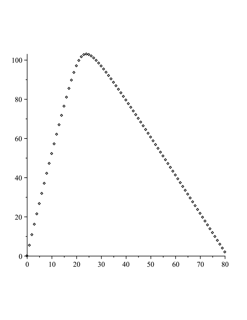
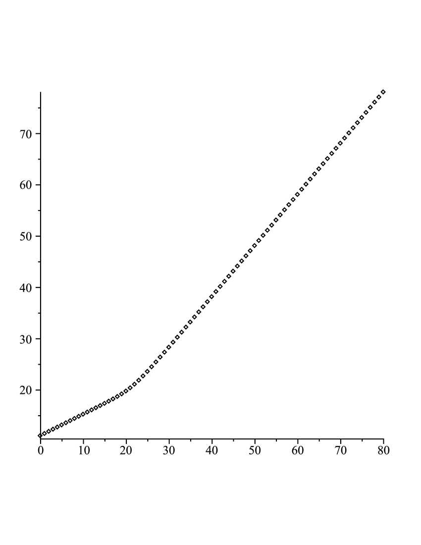
Figure 1: Recurrence coefficients ($a_{n}^{2}$ on the left, $b_{n}$ on the right) for generalized Krawtchouk polynomials ($N=80$, $\alpha=-1$, $c=2$)

Figure 2: Recurrence coefficients ($a_{n}^{2}$ on the left, $b_{n}$ on the right) for generalized Krawtchouk polynomials ($N=80$, $\alpha=0.8$, $c=2$).

4 Computing the recurrence coefficients

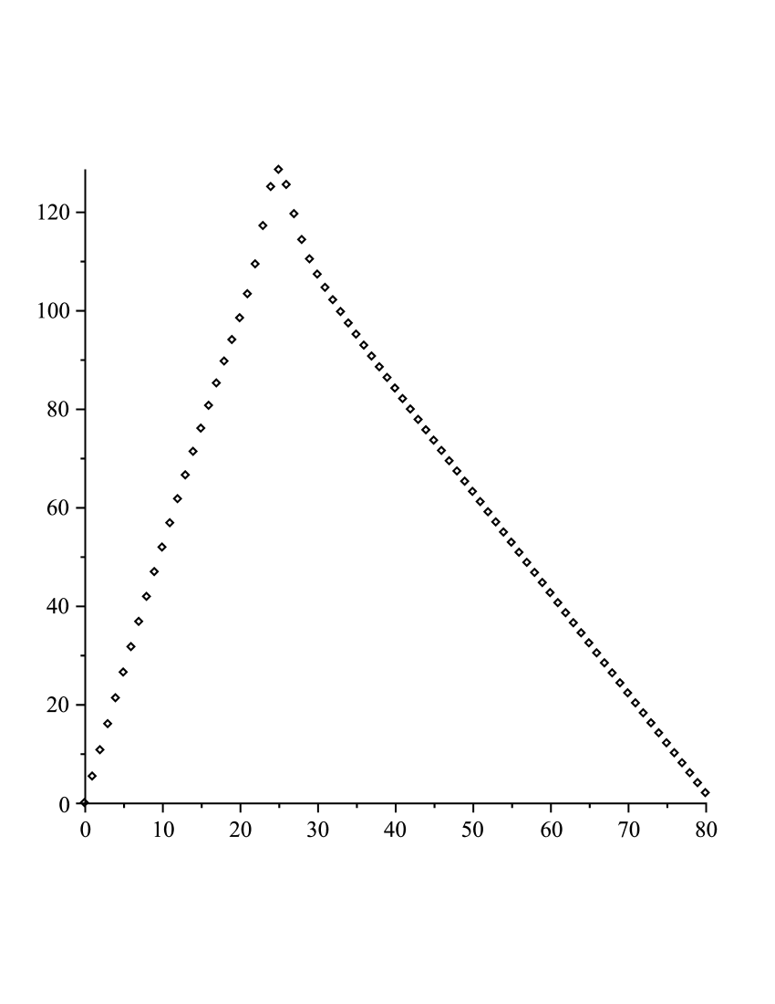
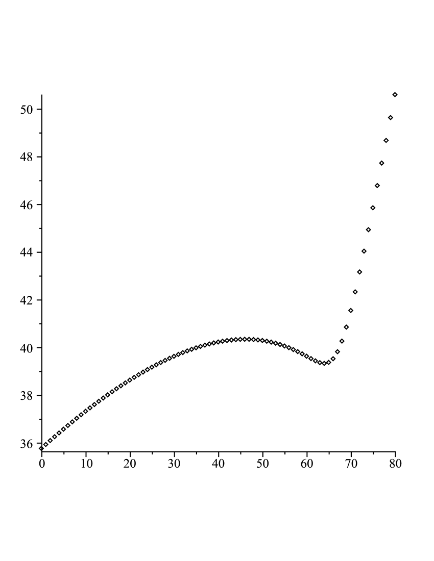
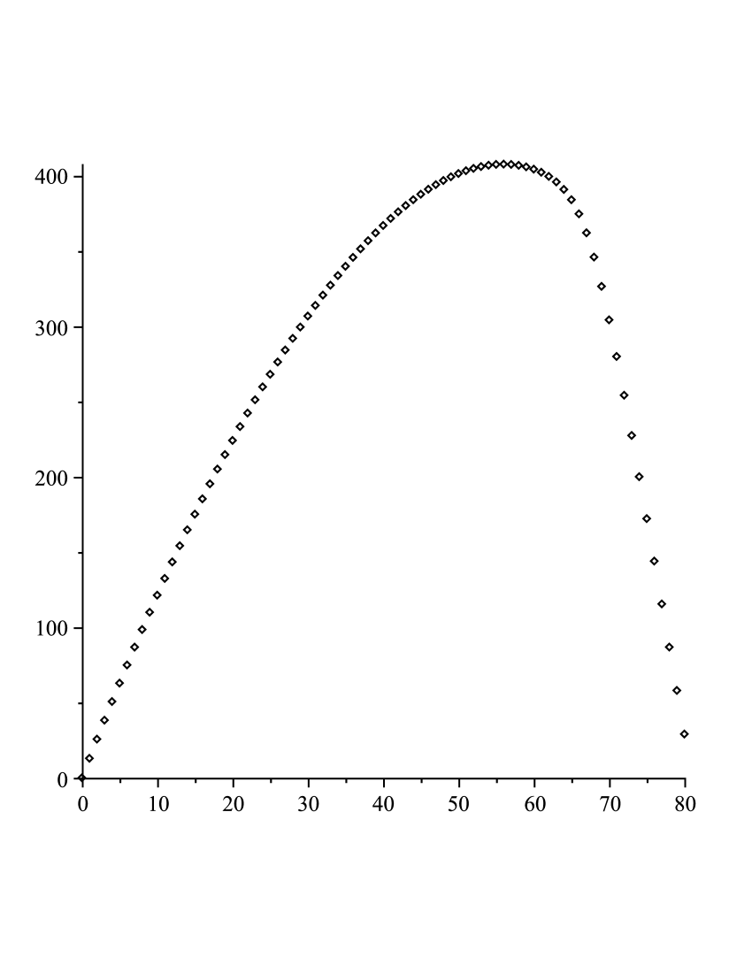
Figure 3: Recurrence coefficients ($a_{n}^{2}$ on the left, $b_{n}$ on the right) for generalized Krawtchouk polynomials ($N=80$, $\alpha=-1$, $c=30$).

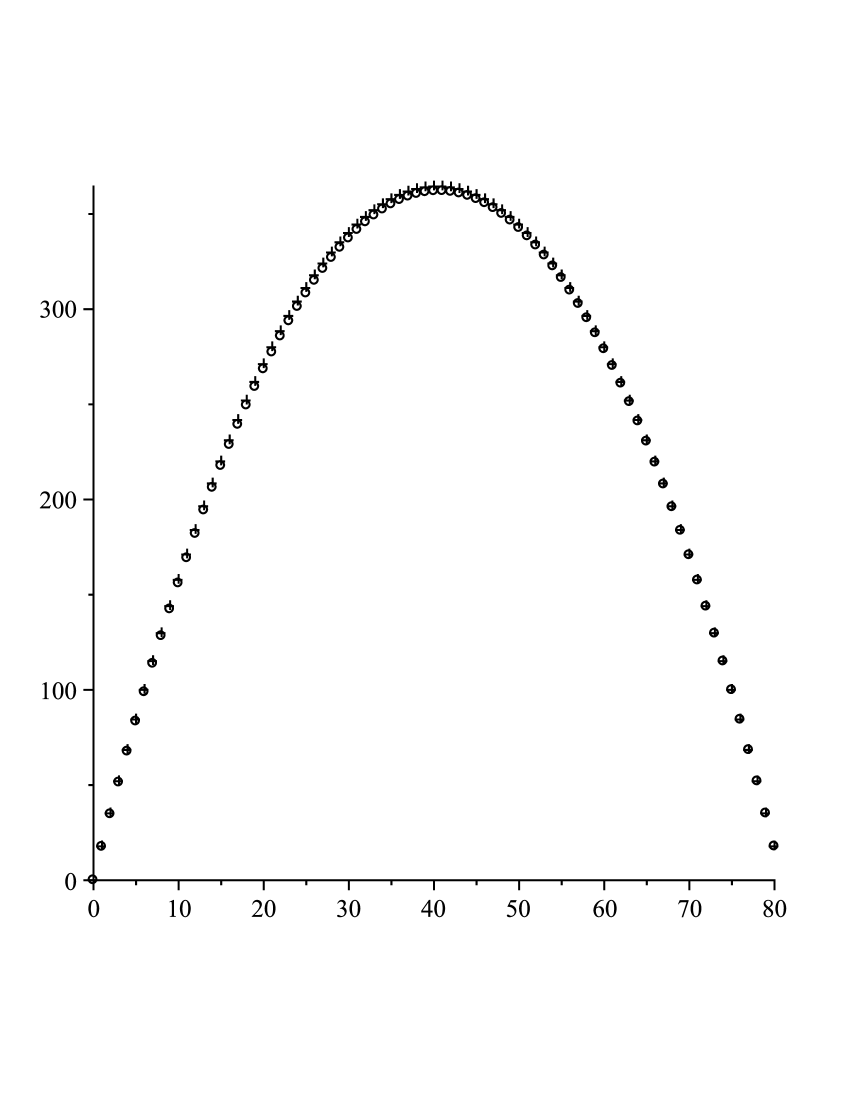
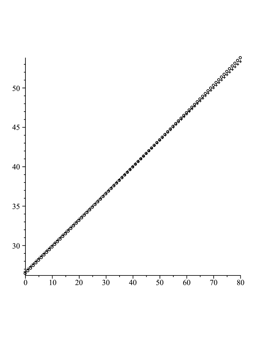
Figure 4: Recurrence coefficients ($a_{n}^{2}$ on the left, $b_{n}$ on the right) for generalized Krawtchouk polynomials ($N=80$, $\alpha=-2000$, $c=1000$, circles) and for Krawtchouk polynomials ($N=80$, $p=1/3$, crosses)

The system (1.10), together with the definitions (1.8) and (1.9), can be used to compute the recurrence coefficients starting with the initial values $x_{0}$ and $y_{0}$ given in (1.11). Figures 1-3 show these coefficients for $N=80$ and for some different choices of the parameters $c>0$ and $\alpha<1$. Recall that the recurrence coefficients (1.6) for the Krawtchouk polynomials are such that $a_{n}^{2}$ is quadratic in $n$, with $a_{0}^{2}=0=a_{N+1}^{2}$, and that $b_{n}$ is of degree 1 in $n$. Also recall that when $c$ and $-\alpha$ tend to infinity and $-\frac{c}{\alpha}\to\frac{p}{1-p}$ we recover the Krawtchouk weight. Figure 4 shows this observation. For the generalized Krawtchouk polynomials the $a_{n}^{2}$ are first increasing until they reach their maximum, and then decreasing, with $a_{0}^{2}=0=a_{N+1}^{2}$. The $b_{n}$ are no longer linear but change from concave to convex. The point where $a_{n}^{2}$ reaches its maximum and the inflection point for the $b_{n}$ depend on the parameter $c$, these two points do not coincide. Moreover, for $\alpha$ values close to $1$, the $b_{n}$ change once more to concave, as can be seen (albeit not very clearly) in Figure 2.

To get these values (they were obtained using Maple), one has to work with quite high accuracy, for it turns out that even a very small perturbation ($10^{-100}$ for $N=80$) in the initial value $y_{0}$ quickly leads to very bad results. An explanation for this behaviour is the following: the system (1.10) allows to compute the $x_{n}$, from which the coefficients $a_{n}^{2}$ can be obtained by (1.8). There is, however, no a priori reason why these $a_{n}^{2}$ should be positive and $a_{N+1}^{2}=0$. This is not a new observation: in [1] (Section 6.5, about discrete $q$-Hermite I polynomials) it was conjectured that the initial value needed to obtain the recurrence coefficients for these polynomials, is the only real value which leads to positive values for $a_{n}^{2}$ for every $n>0$. Since in this generalized Krawtchouk case there is only a finite number of coefficients ($a_{1}^{2},\ldots,a_{N}^{2}$) which need to be positive, this conjecture obviously does not hold here, but we conjecture that there is only one initial value $y_{0}$ for which $a_{N+1}^{2}=0$ and the $a_{1}^{2},\ldots,a_{N}^{2}$ are positive. An alternative, and numerically more stable way, would be to use a fixed point algorithm for which the fixed point satisfies (1.10).

Following a referee’s remark, we also used the Stieltjes approach to calculate the recurrence coefficients, see e.g. [14, §2.2.3.1]. In this method, one uses (1.3) to calculate $a_{n}$ and $b_{n}$ from $p_{n}$ and $p_{n-1}$. Then (1.2) can be used to obtain $a_{n+1}p_{n+1}(x)$, which after normalization gives $p_{n+1}$. The initial values needed are $p_{-1}=0$ and $p_{0}=\frac{1}{\sqrt{\sum_{k=0}^{N}w(k)}}$. Numerical calculations show that this method needs less precision in the initial conditions but requires more computations.

5 Conclusion and future directions

In this paper we have been dealing with the recurrence coefficients of the discrete orthogonal polynomials, namely the generalized Krawtchouk polynomials, and have shown that they are related to the classical solutions (in terms of confluent hypergeometric functions) of the fifth Painlevé equation. A possible further direction is to consider more factors in (2.9) and find out whether the sixth Painlevé equation or some equation from the Painlevé hierarchy is related to the recurrence coefficients of such a weight. A reason that leads to this conjecture follows from the observation that the initial conditions for such a weight correspond to special solutions of the sixth Painlevé equation.

Galina Filipuk
Faculty of Mathematics, Informatics and Mechanics
University of Warsaw
Banacha 2 Warsaw 02-097, Poland
filipuk@mimuw.edu.pl


Lies Boelen, Christophe Smet, Walter Van Assche, Lun Zhang
Department of Mathematics
KU Leuven
Celestijnenlaan 200 B box 2400
BE-3001 Leuven
Belgium
lies.boelen@gmail.com
christophe@wis.kuleuven.be
walter@wis.kuleuven.be
lun.zhang@wis.kuleuven.be

References

• [1] L. Boelen, Discrete Painlevé Equations and Orthogonal Polynomials, Ph.D. diss., Department of Mathematics K.U.Leuven, Leuven, Belgium, 2010.
• [2] L. Boelen, G. Filipuk, and W. Van Assche, Recurrence coefficients of generalized Meixner polynomials and Painlevé equations, J. Phys. A: Math. Theor. 44 (2011), 035202 (19p).
• [3] L. Boelen and W. Van Assche, Discrete Painlevé equations for recurrence coefficients of semiclassical Laguerre polynomials, Proc. Amer. Math. Soc. 138 (2010), pp. 1317–1331.
• [4] T.S. Chihara, An Introduction to Orthogonal Polynomials, Gordon and Breach, New York, 1978.
• [5] P.A. Clarkson, Special polynomials associated with rational solutions of the fifth Painlevé equation, J. Comput. Appl. Math. 178 (2005), pp. 111–129.
• [6] P.A. Clarkson, Painlevé Equations–Nonlinear Special Functions, Lecture Notes in Mathematics, vol. 1883, Berlin: Springer, 2006, pp. 331–411.
• [7] C.M. Cosgrove, Chazy’s second-degree Painlevé equations, J. Phys. A: Math. Gen. 39 (2006), pp. 11955-11971.
• [8] Digital Library of Mathematical Functions, National Institute of Standards and Technology, http://dlmf.nist.gov/
• [9] G. Filipuk and W. Van Assche, Recurrence coefficients of generalized Charlier polynomials and the fifth Painlevé equation, Proc. Amer. Math. Soc. DOI:10.1090/S0002-9939-2012-11468-6.
• [10] G. Filipuk and W. Van Assche, Recurrence coefficients of a new generalization of the Meixner polynomials, SIGMA 7 (2011), 068 (11p).
• [11] G. Filipuk, W. Van Assche, and L. Zhang, The recurrence coefficients of semi-classical Laguerre polynomials and the fourth Painlevé equation, J. Phys. A: Math. Theor 45 (2012), 205201 (13pp).
• [12] P.J. Forrester and N.S. Witte, Application of the τ𝜏\tau-function theory of Painlevé equations to random matrices: PVsubscriptPV\rm P_{V}, PIIIsubscriptPIII\rm P_{III}, the LUE, JUE, and CUE, Comm. Pure Appl. Math. 55 (2002), pp. 679–727.
• [13] B. Gambier, Sur les équations différentielles du second ordre et du premier degré dont l’intégrale générale est à points critiques fixés, Acta Math. 33 (1910), pp. 1–55.
• [14] W. Gautschi, Orthogonal Polynomials: Computation and Approximation, Numerical Mathematics and Scientific Computation, Oxford University Press, 2004.
• [15] B. Grammaticos and A. Ramani, Discrete Painlevé equations: a review, Lect. Notes Phys., 644, Springer, 2004, pp. 245–321.
• [16] V.I. Gromak, The solutions of Painlevé’s fifth equation, Differential Equations 12 (1976), pp. 519–521.
• [17] V.I. Gromak, I. Laine, and S. Shimomura, Painlevé Differential Equations in the Complex Plane, Studies in Mathematics 28, de Gruyter, Berlin, 2002.
• [18] E. Hendriksen and H. van Rossum, Semi-classical orthogonal polynomials, in Polynômes Orthogonaux et Applications, Lect. Notes in Math. 1171, Springer-Verlag, Berlin, 1985, pp. 354–361.
• [19] M.E.H. Ismail, Classical and Quantum Orthogonal Polynomials in One Variable, Encyclopedia of Mathematics and its Applications 98, Cambridge University Press, 2005.
• [20] M.E.H. Ismail, I. Nikolova, and P. Simeonov, Difference equations and discriminants for discrete orthogonal polynomials, Ramanujan J. 8 (2004), pp. 475–502.
• [21] A.V. Kitaev, C.K. Law, and J.B. McLeod, Rational solutions of the fifth Painlevé equation, Differential Integral Equations 7 (1994), pp. 967–1000.
• [22] A.P. Magnus, Freud’s equations for orthogonal polynomials as discrete Painlevé equations, in Symmetries and Integrability of Difference Equations, London Math. Soc. Lecture Note Ser. 255, Cambridge University Press, 1999, pp. 228–243.
• [23] P. Maroni, Prolégomènes à l’étude des polynômes orthogonaux semi-classiques, Ann. Mat. Pura Appl. 149 (1987), pp. 165–184.
• [24] T. Masuda, Classical transcendental solutions of the Painlevé equations and their degeneration, Tohoku Math. J. 56 (2004), pp. 467–490.
• [25] T. Masuda, Y. Ohta, and K. Kajiwara, A determinant formula for a class of rational solutions of Painlevé V equation, Nagoya Math. J. 168 (2002), pp. 1–25.
• [26] A.F. Nikiforov, S.K. Suslov, and V.B. Uvarov, Classical Orthogonal Polynomials of a Discrete Variable, Springer Series in Computational Physics, Springer-Verlag, Berlin, 1991.
• [27] M. Noumi and Y. Yamada, Umemura polynomials for the Painlevé V equation, Phys. Lett. A 247 (1998), pp. 65–69.
• [28] K. Okamoto, Studies on the Painlevé equations. II. Fifth Painlevé equation PVV{}_{\textup{V}}, Japan. J. Math. (N.S.) 13 (1987), pp. 47–76.
• [29] P. Painlevé, Mémoire sur les équations différentielles dont l’intégrale générale est uniforme, Bull. Soc. Math. Phys. Fr. 28 (1900), pp. 201–61.
• [30] P. Painlevé, Sur les équations différentielles du second ordre et d’ordre supérieure dont l’intégrale générale est uniforme, Acta Math. 21 (1902), pp. 1–85.
• [31] C. Smet and W. Van Assche, Orthogonal polynomials on a bi-lattice, Constr. Approx. 36 (2) (2012), pp. 215–242.
• [32] W. Van Assche, Discrete Painlevé equations for recurrence coefficients of orthogonal polynomials, in Difference Equations, Special Functions and Orthogonal Polynomials (S. Elaydi et al., eds.), World Scientific, 2007, pp. 687–725.
• [33] H. Watanabe, Solutions of the fifth Painlevé equation. I., Hokkaido Math. J. 24 (1995), pp. 231–267.