All sky CMB map from cosmic strings integrated Sachs-Wolfe effect

Abstract

By actively distorting the cosmic microwave background (CMB) over our past light cone, cosmic strings are unavoidable sources of non-Gaussianity. Developing optimal estimators able to disambiguate a string signal from the primordial type of non-Gaussianity requires calibration over synthetic full sky CMB maps, which untill now had been numerically unachievable at the resolution of modern experiments. In this paper, we provide the first high resolution full sky CMB map of the temperature anisotropies induced by a network of cosmic strings since the recombination. The map has about 200 million sub-arcminute pixels in the healpix format which is the standard in use for CMB analyses ($N_{\mathrm{side}}=4096$). This premiere required about 800,000 cpu hours; it has been generated by using a massively parallel ray tracing method piercing through thousands of state of art Nambu-Goto cosmic string numerical simulations which pave the comoving volume between the observer and the last scattering surface. We explicitly show how this map corrects previous results derived in the flat sky approximation, while remaining completely compatible at the smallest scales.

I Introduction

As all topological defects Kibble (1976), cosmic strings incessantly generate gravitational perturbations all along the universe history Pen et al. (1997); Durrer and Kunz (1998); Durrer and Zhou (1996). Their amplitude is directly given by the string energy density per unit length, $GU\ll 1$ (in Planck unit), which is also the typical energy scale at which these objects are formed, eventually redshifted by warped extra-dimension for the so-called cosmic superstrings Copeland et al. (2004); Davis and Kibble (2005); Sakellariadou (2009); Copeland and Kibble (2010). Although the theory of cosmological perturbations can be applied to defects Durrer et al. (2002), predicting string induced anisotropies in the CMB is challenging. As opposed to the perturbations of inflationary origin, which are generated once and for all in the early universe, active sources require the complete knowledge of their evolution at all times, from their formation till today Pen et al. (1994); Magueijo et al. (1996a, b); Achucarro et al. (1999); Contaldi et al. (1999).

For these reasons, cosmological analyses often rely on analytical, or semi-analytical defect models Pogosian and Vachaspati (1999); Gangui et al. (2001); Siemens et al. (2006); Jeong and Smoot (2007); Pogosian and Wyman (2008); Pshirkov and Tuntsov (2010); Danos and Brandenberger (2010); Tuntsov and Pshirkov (2010); Danos et al. (2010); Demorest et al. (2012); Kamada et al. (2012) which may not be accurate enough in view of the incoming flow of high precision CMB data, such as those from the Planck satellite and the other sub-orbital experiments Huffenberger and Seljak (2005); Ruhl et al. (2004); R. Barker et al. (2006) (AMI Collaboration); Ade et al. (2011). The theoretical understanding of cosmic string evolution in a Friedmann-Lemaître-Robertson-Walker (FLRW) universe is still an active field of research which has led to the development of various theoretical models Austin et al. (1993); Copeland et al. (1998); Martins and Shellard (2002); Polchinski and Rocha (2006); Dubath et al. (2008); Rocha (2008); Copeland and Kibble (2009); Martins (2009); Lorenz et al. (2010); Pourtsidou et al. (2011); Avgoustidis et al. (2011) and numerical simulations, the latter having the advantage of incorporating all the defect dynamics Bennett and Bouchet (1989); Albrecht and Turok (1989); Bennett and Bouchet (1990); Allen and Shellard (1990); Vincent et al. (1998); Moore et al. (2001); Wu et al. (2002); Ringeval et al. (2007); Vanchurin et al. (2005); Olum and Vanchurin (2007); Martins and Shellard (2006); Blanco-Pillado et al. (2011). However, within simulations, the dynamical range remains limited such that one has to extrapolate numerical results over orders of magnitude by means of their scale invariant properties. The CMB temperature and polarization angular power spectra have been derived for local strings only within the Abelian Higgs model Bevis et al. (2007a, b, 2010). As simulations do have only one free parameter that is $GU$, they provide a robust correspondence between string tension and CMB amplitude. From current data, Ref. Urrestilla et al. (2011) reports the two-sigma confidence limit $GU<4.2\times 10^{-7}$, whereas semi-analytical methods find bounds ranging from $10^{-9}$ to $10^{-6}$ Fraisse (2007); Sadegh Movahed and Khosravi (2011); Battye and Moss (2010); Dvorkin et al. (2011).

Among other signatures, non-Gaussianities are unavoidable consequences of the presence of cosmic strings (see Ref. Ringeval (2010); Hindmarsh (2011) for a review). The determination of the power spectrum, i.e. the two-points function, from numerical simulations is not easy, and the situation is even worse for any higher n-point function. A way around this is to include photons inside a string simulation to produce a realization of the expected CMB temperature anisotropies. In that respect, the resulting map contains all the statistical content, non-Gaussianities included. This method has originally been introduced for Nambu-Goto strings in Ref. Bouchet et al. (1988) and revived in Ref. Fraisse et al. (2008) to create a collection of statistically independent small angle CMB maps. As shown by Hindmarsh, Stebbins and Veeraraghavan, the small angle limit happens to be very convenient as the perturbed photon propagation equations, namely the string induced integrated Sachs-Wolfe (ISW) effect Gott III (1985); Kaiser and Stebbins (1984), reduces to a more tractable two-dimensional problem Hindmarsh (1994); Stebbins and Veeraraghavan (1995). Those maps have been shown to be accurate as they correctly reproduce the small scale power spectrum of Abelian strings Bevis et al. (2010) as well as the analytically expected one-point Takahashi et al. (2009); Yamauchi et al. (2010a, b) and higher n-point functions Hindmarsh et al. (2009, 2010); Regan and Shellard (2010). Although flat sky maps are adequate to devise new string-oriented searches in small scale CMB data Hammond et al. (2009); Niemack et al. (2010); Dunkley et al. (2011), current searches for non-Gaussianities are mainly driven by the primordial type and based on full sky optimized estimators Liguori et al. (2010); Regan et al. (2010); Fergusson et al. (2010); Curto et al. (2011) (see Ref. Huterer et al. (2010) for a review).

In this paper, we generalize the method used in Ref. Fraisse et al. (2008) and go beyond the flat sky approximation to generate a full sky CMB map induced by Nambu-Goto strings. The most unequivocal signature from strings are the temperature discontinuities they induce, which are naturally most striking at small scales; our efforts thus have been to achive a high resolution over the complete sky. In a hierarchical equal area isolatitude pixelisation of the sky, we have been able to maintain an angular resolution of $\theta_{\mathrm{res}}=0.85^{\prime}$, i.e. using the publicly available HEALPix code Gorski et al. (2005), our map has $N_{\mathrm{side}}=4096$, i.e. $2\times 10^{8}$ pixels. As detailed in the following, our method includes all string effects from the last scattering surface till today, but does not include the Doppler contributions induced by the strings into the plasma prior to recombination. As a result, our map represents the ISW contribution from strings, which is dominant at small scales but underestimates the signal on intermediate length scales. Including the Doppler effects requires the addition of matter in the simulations, an approach which has been implemented in Refs. Landriau and Shellard (2003, 2004) and recently used to generate a full sky map in Ref. Landriau and Shellard (2011). As discussed in that reference, the computing resources required to include matter severely limit the achievable resolution to $14^{\prime}$ ($N_{\mathrm{side}}=256$, with 800 000 pixels). In that respect, our map is complementary to the one of Ref. Landriau and Shellard (2011) while extending the domain of applicability of existing small angle maps Fraisse et al. (2008). In particular, we recover the turnover in the spectrum observed around $\ell\simeq 200$ in Ref. Landriau and Shellard (2011), which was cut by the small field of view of the flat sky maps.

The paper is organized as follows. In Sec. II, we briefly recap the characteristics of our numerical simulations of cosmic string networks and describe the ray tracing method used to compute the full sky map. The map itself is presented in Sec. III and compared with the small angle maps in the applicable limit. We also compute the angular power spectrum and conclude in the last section.

II Method

II.1 All sky string ISW

Denoting by $X^{\mu}(\tau,\sigma)$ the string embedding functions, in the transverse temporal gauge, up to a dipole term, the integrated Sachs–Wolfe contribution sourced by the Nambu-Goto stress tensor reads Stebbins and Veeraraghavan (1995)

$$\Theta(\boldsymbol{\hat{n}})=-4GU\int_{\boldsymbol{X}\,\cap\,\boldsymbol{x}_{\gamma}}\negthickspace\negthickspace\negthickspace\negthickspace\boldsymbol{u}\cdot\dfrac{X\boldsymbol{\hat{n}}-\boldsymbol{X}}{\left(X\boldsymbol{\hat{n}}-\boldsymbol{X}\right)^{2}}\,\epsilon\,\mathrm{d}\sigma,$$ (1)

where $\Theta(\boldsymbol{\hat{n}})$ stands for the relative photon temperature shifts ($\Theta\equiv\Delta T/T$) in the observation direction $\boldsymbol{\hat{n}}$. The integral is performed over all string position vectors $\boldsymbol{X}=\{X^{i}\}$ intercepting our past line cone, the invariant string length element being $\mathrm{d}l=\epsilon\mathrm{d}\sigma$ with $\epsilon^{2}\equiv\boldsymbol{\acute{X}}^{2}/(1-\boldsymbol{\dot{X}}^{2})$. The string dynamical effects are encoded in

$$\boldsymbol{u}=\boldsymbol{\dot{X}}-\dfrac{(\boldsymbol{\hat{n}}\cdot\boldsymbol{\acute{X}})\cdot\boldsymbol{\acute{X}}}{1+\boldsymbol{\hat{n}}\cdot\boldsymbol{\dot{X}}},$$ (2)

where the “acute accent” and the “dot” denote differentiation with respect to the world sheet coordinates $\sigma$ and $\tau$, respectively. The small angle and flat sky approximations consists in taking the limit $X\boldsymbol{\hat{n}}\rightarrow\boldsymbol{X}$ which assumes that the observation direction matches with the string location and that all photon trajectories are parallel Hindmarsh (1994); Bouchet et al. (1988); Fraisse et al. (2008). Let us notice that Eq. (1) cannot be applied to a straight static string, but such a situation never occurs for the realistic string configurations studied in the following Stebbins and Veeraraghavan (1995); Veeraraghavan and Stebbins (1992).

In the following, we use the all sky expression of Eq. (1) to compute the induced temperature anisotropies $\Theta(\boldsymbol{\hat{n}})$ in each of the wanted $2\times 10^{8}$ pixelized directions. Equation (1) shows that, in each direction, one has to sum up the contribution of all string segments $\mathrm{d}l$ intercepting our past light cone since the last scattering surface and determine, for each of them, $\boldsymbol{\acute{X}}$ and $\boldsymbol{\dot{X}}$. Although one string lying behind the observer does not contribute more than a few percent to the overall signal, it is impossible to artificially cut it without adding spurious discontinuities in the map, which would dangerously mimic real string patterns. As discussed below, we have filled the comoving volume between today and the last scattering surface with a few thousand Nambu-Goto numerical simulations in Friedmann-Lemaître-Robertson-Walker (FLRW) space-time. Typically, hundreds of millions of string segments intercept on our past light cone, each of them has to be included in Eq. (1) to get the overall signal for one pixel. One can immediately understand the computing challenge to obtain a full sky map as the total number of expected iterations roughly sums up to $10^{16}$.

II.2 Nambu-Goto string simulations

In order to get a realistic string configuration between the last scattering surface and today, we have followed Refs. Bouchet et al. (1988); Fraisse et al. (2008) and stacked FLRW string simulations using an improved version of the Bennett and Bouchet Nambu-Goto cosmic string code Bennett and Bouchet (1990); Ringeval et al. (2007). The runs have the same characteristics as those used in Ref. Fraisse et al. (2008) and, in particular, we include only the loops having a size larger than a time-dependent cut-off. The reason being that loops smaller than this cut-off have a distribution which is known to be contaminated by relaxation effects from the numerical initial conditions. As explained in Ref. Fraisse et al. (2008), the cutoff is dynamically chosen by monitoring the time evolution of the energy density distribution associated with loops of different sizes. This ensures that we include only loops having an energy density evolving as in scaling, i.e. in $1/t^{2}$. One may be worried about the deficit due to the missing loops artificially removed by the cut-off. An upper bound of the systematic errors that could be induced by these relaxation effects can be found in that same reference (see Sec. II.D). It does not exceed $10\%$ on average and concerns only very small scales. In the following, we recap some of the relevant physical properties underlying our numerical simulations (see Sec. II.B in Ref. Fraisse et al. (2008) for more details). Each simulation allows one to trace the time evolution of a network of cosmic strings in scaling over a cubic comoving volume of typical size

$$L_{\mathrm{sim}}\simeq 30\dfrac{1-\sqrt{\Omega_{\mathrm{rad}}/\Omega_{\mathrm{mat}}}\sqrt{1+z_{\mathrm{i}}}}{h\sqrt{\Omega_{\mathrm{mat}}}\sqrt{1+z_{\mathrm{i}}}}\,\textrm{Gpc}.$$ (3)

In this expression, $z_{\mathrm{i}}$ is the redshift at which the simulation is started, $h$ is the reduced Hubble parameter today and $\Omega_{\mathrm{mat}}$, $\Omega_{\mathrm{rad}}$ are the density parameters of matter and radiation today. Starting at the last scattering surface, $z_{\mathrm{i}}=1089$, gives a simulation comoving box of $L_{\mathrm{sim}}\simeq 1.7\,\textrm{Gpc}$, which corresponds to an angular size of $7.2^{\circ}$. At the same time strings are evolved, we propagate photons along the three spatial directions and record all $\boldsymbol{\acute{X}}$ and $\boldsymbol{\dot{X}}$ for each string segment intercepting those light cones. Depending on the simulation realization, and its location, this corresponds to typically $10^{4}$–$10^{5}$ projected string segments. One run is limited in time, as we use periodic boundary conditions, and ends after a 30-fold increase in the expansion factor, i.e. at a redshift $z_{\mathrm{e}}=36$. As a result, covering the whole sky requires stacking side-by-side many different simulations, all starting at $z_{\mathrm{i}}=1089$ and ending at $z_{\mathrm{e}}=36$. The missing redshift range can be dealt exactly in the same manner by stacking another set of runs which start at $z_{\mathrm{i}}=36$ and end at $z_{\mathrm{e}}=0.2$. From Eq. (3), we see that the low-redshift simulations have a size of $L_{\mathrm{sim}}\simeq 13\,\textrm{Gpc}$ such that only a few of them are required to cover the whole comoving volume. Notice that the use of different simulations to fill the comoving space does not induce visible artifacts in the final map. The signal being only sourced by the subset of string segments intercepting the past light cone, the probability of seeing an edge is almost vanishing. Finally, as in Ref. Fraisse et al. (2008), we have skipped the last interval from $z=0.2$ to $z=0$ as almost no string intercepts our past line cone in that range.

In the next section, we describe in more detail how we cut and stack the cosmic string simulations.

II.3 Stacking simulations with healpix cones

The hierarchical equal area iso-latitude pixelisation (healpix) of the two-sphere is a efficient method to pixelize the sky which is well-suited to and commonly used for CMB analysis Gorski et al. (2005). Our stacking method relies on the voxelization of the three-dimensional ball using cones subtending healpix pixels on its boundaries, i.e. for the two redshifts at which we start and stop the numerical simulations. For the high-redshift contributions, the healpix cones fill the whole spherical volume in between the last scattering surface at $z_{\mathrm{i}}=1089$ and the two-sphere at $z_{\mathrm{e}}=36$ (see Fig. 1). The rest of the volume, associated with the low redshift simulations, can be voxelized exactly in the same way but starting on the two-sphere at $z_{\mathrm{i}}=36$ and ending at $z_{\mathrm{e}}=0.2$. The actual string dynamics simulations are evolved in cubic comoving boxes in which we take only strings living inside a healpix cone. In order to minimize the number of simulations required, the problem is now reduced to find the largest healpix cone fitting inside a cubic comoving box for all redshifts of interest. Moreover, one has to ensure that the photons intercepting the strings travel towards the observer. As seen in Fig. 1, both requirements can be implemented by adequately rotating the simulation box such that photons face the observer line of sight $\boldsymbol{\hat{n}}$, and the farthest healpix pixel fits inside the farthest squared face of the simulation box. As we propagate three photon waves in each simulation, one can use the same simulation rotated three times. Keeping only the strings living inside the healpix cones, one needs to patch them up till the whole comoving volume is filled. For this purpose, we have used the algorithms implemented within the HEALPix library Gorski et al. (2005).

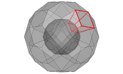
Figure 1: Voxelization of the comoving space between the two redshifts at which cosmic string simulations start and stop, here $z_{\mathrm{i}}=1089$ (outer sphere) and $z_{\mathrm{e}}=36$ (inner sphere). All strings living in each healpix cone are kept and stacked to fill the whole comoving volume. Our high redshift voxelization scheme uses $N_{\mathrm{side}}^{\mathrm{hz}}=16$, i.e. requires $3072$ string simulations while the low redshift one, starting at $z_{\mathrm{i}}=36$ and ending now, has $N_{\mathrm{side}}^{\mathrm{lz}}=1$, i.e. $12$ simulations.

For the high-redshift contribution, the above requirements are satisfied with a healpix voxelization having $N_{\mathrm{side}}^{\mathrm{hz}}=16$, i.e. $3072$ truncated cones from $z=1089$ to $z=36$, therefore calling for $3072$ cosmic string runs. As we can use one run three times, we have only performed $1024$ independent simulations as described in Sec. II.2 (and Ref. Fraisse et al. (2008)). Concerning the low-redshift contribution, the simulation volume $L_{\mathrm{sim}}$ being much larger, $N_{\mathrm{side}}^{\mathrm{lz}}=1$ or $12$ simulations are enough to cover the volume. Let us emphasize, at this stage, that the above-mentioned HEALPix resolutions only concern the simulation stacking method. In the next section, we discuss how we discretize the CMB sky using another, but more conventional, healpix scheme.

II.4 Healpix sky

Assuming we have stacked the cosmic string simulations as previously explained, we have at our disposal a realization of all $\boldsymbol{\dot{X}}$ and $\boldsymbol{\acute{X}}$ lying on our past light cone since the last scattering surface. From Eqs. (1) and (2), the remaining step is to actually perform the integral for each desired value of the observer direction $\boldsymbol{\hat{n}}$. Choosing the values of $\boldsymbol{\hat{n}}$ has been made by using another healpix pixelization scheme, this time on the simulated sky. A typical Planck-like CMB experiment requiring an angular resolution of $5^{\prime}$, we have chosen an angular resolution of $0.9^{\prime}$ to reduce sufficiently the small scale inaccuracies which are present at the subpixel scale. The corresponding healpix resolution is $N_{\mathrm{side}}=4096$, i.e. a sky map having $2\times 10^{8}$ pixels.

In the next section, after having briefly exposed how the above computing challenges have been solved, we present the simulated CMB map.

III String sky map

The method we have exposed in the previous section has the advantage to be completely factorizable into two independent numerical problems. The first is to perform string simulations and record only those events intercepting the light cones. The second is to use these events to actually perform the integration of Eq. (1), which gives the final signal $\Theta(\boldsymbol{\hat{n}})$.

III.1 Computing resources

Performing the one thousand cosmic string runs has required around $300,000$ cpu-hours on current x86-64 processors. The needed memory and disk space resources remaining reasonable, the computations have used local computing resources provided by the Planck-HFI computing centre at the “Institut d’Astrophysique de Paris” and the CP3 cosmo cluster at Louvain University. By the end of the runs, the total number of string segments recorded on the light cone account for typically $1\,\textrm{Tb}$ of storage data.

From the light cone data, performing $2\times 10^{8}$ line of sight integrals over $10^{8}$ string segments [see Eq. (1)] is a serious numerical problem. This part of the code has therefore been parallelized at three levels using the symmetries of the problem.

First, we have used a distributed memory parallelization as implemented in the message passing interface (MPI) to split the string contributions into sub-blocks. From our previous discussing, a natural implementation is an MPI-parallelization over the healpix cones which therefore allows different machines to deal with a subset of cones. More intuitively, it means that the final map is obtained by adding up full sky maps, each one being sourced by the strings contained in a few healpix cones only. Second, for each of those processes, the computation of the $2\times 10^{8}$ pixels has been parallelized using the shared memory OpenMP directives. In other words, pixels can be simultaneously computed using all of the available processors inside a single machine. Finally, for each of the above OpenMP threads, we have vectorized the most inner loop, i.e. the discrete version of Eq. (1). Doing this allows to use simultaneously multiple registers of each processing unit to add up a few string segments at once.

The computing resources have been provided by the National Energy Research Scientific Computing Center (NERSC) at the Lawrence Berkeley National Laboratory. The run has been performed on the hopper super-computer using $512$ MPI nodes at the first level of parallelization. On each node, we have deployed the OpenMP parallelization over the $24$ cores available. Each node is made of two twelve-cores “AMD MagnyCours” cpus which supports only a limited amount of vectorization. However, a vectorization over $16$ string segments significantly improves cache memory latency and gives a final speed-up of two compared to a pure scalar processing. All in all, the whole computation required $12,000$ cores and has been completed after $500,000$ cpu-hours.

III.2 Results

In Fig. 2, we have plotted the final map together with the two contributions coming from high and low redshift. As expected, most of the strings are at high redshift, the low redshift contribution showing only a few strings crossing the sky. For this reason, we have not included strings with $z<0.2$, as almost no strings are present.

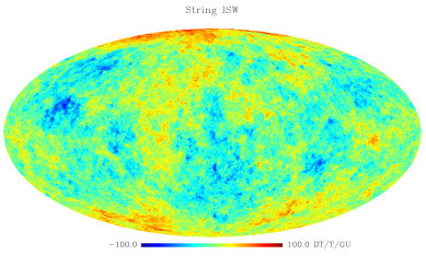
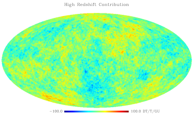
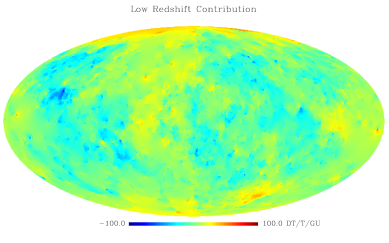
Figure 2: All sky CMB map of string induced ISW effect (upper panel) in a Mollweide projection. The two lower maps represent respectively the high redshift contribution (from last scattering to $z=36$) and the low redshift contribution (from $z=36$ to now). The color scale indicates the range of $\Theta/GU$ fluctuations which, once multiplied by the value of $GU$ and $T_{\mathrm{{\scriptscriptstyle{CMB}}}}$, would thus be in the tens of $\mu\mathrm{K}$ range for $GU\sim 10^{-6}$.

At first glance these maps may look Gaussian, which is because the string patterns essentially show up at small scales while they are averaged on the largest angular scales Landriau and Shellard (2011). In Fig. 3, we have represented a zoom over a $7.2^{\circ}$ region in which one recovers the same string discontinuities as previously derived within the flat sky approximation Fraisse et al. (2008). In order to make the comparison sharper, both the gnomic projection of our spherical patch and the flat sky map coming from the same string simulation are represented in Fig. 3. Up to some spherical distortions off-center, both maps predict the same structures.

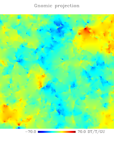
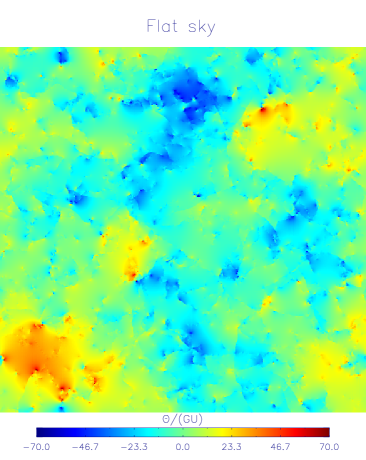
Figure 3: Comparison between full sky and flat sky / small angle approximation. The upper panel is a gnomic projection of a $7.2^{\circ}$ patch cut from the high redshift full sky map at the north pole. The lower panel is from Ref. Fraisse et al. (2008) and represents the high redshift flat sky calculation coming from the same string simulation. Both maps exhibit globally the same anisotropy patterns and amplitude. More precisely, there is essentially no difference in the center, whereas geometrical and amplitude distortions become increasingly apparent towards the edges. This is expected as spherical effects are not included in the flat sky approximation.

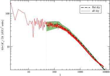
Figure 4: Angular power spectrum extracted from the string map of Fig. 2 (solid red curve) compared to the one estimated in Ref. Fraisse et al. (2008), using the small angle and flat sky approximation (dashed black curve). The shaded region represents the one-sigma fluctuations over various string realizations (flat sky).

Finally, in Fig. 4, we have plotted the angular power spectrum obtained from the full sky map. In this figure, the dashed curve represents the mean value previously derived using flat sky patches in Ref. Fraisse et al. (2008). We observe a very small loss of power compared to the flat sky result, which may not be significant as it does not exceed the one-sigma fluctuations expected between various string realizations. However, as Fig. 3 suggests, the flat sky maps are a bit sharper than the spherical ones due to some missing spherical effects and, as such, they may slightly overestimate the signal. This is not surprising as the flat sky maps are derived using the small angle approximated version of Eq. (1) where all scalar products are postulated to be either parallel or null Hindmarsh (1994). As our full sky map does not approximate anything, it should contain slightly less power.

Let us also notice that there is some extra power for $\ell>5000$ associated with the full sky power spectrum. This is a spurious aliasing effect coming from the slow decrease of the power spectrum at small scales combined with our ray tracing method. Each pixel of the map represents the real signal, but only in the centroid direction $\boldsymbol{\hat{n}}$. This has the effect of including string structures smaller than the pixel angular resolution thereby aliasing the final map.

In Fig. 4, the power spectrum turns-over for $\ell<200$ as those modes correspond to wavelengths larger than the correlation length at recombination. This property was also observed in the map derived in Ref. Landriau and Shellard (2011) but barely visible in the flat sky maps of Ref. Fraisse et al. (2008) due to their small field of view. We see, a posteriori, that this effect was however indeed present as the dash curve of Fig. 4 flattens at the same location than the full sky spectrum.

IV Conclusion

The main result of this article is the map displayed in Fig. 2 which provides a realization of the all sky CMB temperature anisotropies induced by a network of cosmic strings since the last scattering surface. The challenges underlying this map come from both the requirement of covering the whole sky and an unprecedented angular resolution of $0.85$ minute of arc, associated with a HEALPix resolution of $N_{\mathrm{side}}=4096$. However our map includes only the ISW string contribution. This is the dominant signal at small scales, but it misses the Doppler effects around the intermediate multipoles. As those effects have been computed in Ref. Landriau and Shellard (2011), at the expense of having a poor resolution, it will be interesting to investigate whether both results can be combined to obtain a fully accurate representation of the stringy sky over the full range of observable scales.