1 Introduction
Partial differential equations with singularities (PDEwS) have numerous applications in real life processes [1,2]. Most famous equation of this kind is Chaplygin’s equation [3], which can be written as
K ( y ) u x x + u y y = 0 𝐾 𝑦 subscript 𝑢 𝑥 𝑥 subscript 𝑢 𝑦 𝑦 0 K(y)u_{xx}+u_{yy}=0
or in some particular cases as
u x x + u y y + 1 3 y u y = 0 . subscript 𝑢 𝑥 𝑥 subscript 𝑢 𝑦 𝑦 1 3 𝑦 subscript 𝑢 𝑦 0 u_{xx}+u_{yy}+\frac{1}{3y}u_{y}=0.
Latter one called as Tricomi’s equation and was studied well by many authors [4-7]. Due to possible applications and natural mathematical interests for generalization, (PDEwS) were studied intensively and investigations are still going on. One can find bibliographic information on this in the monographs [8-10].
Omitting huge amount works, devoted to investigations of boundary problems and potentials for two dimensional cases of aforementioned equations, note works by A.V.Bitsadze [11], A.M.Nakhushev [12], M.S.Salakhitdinov and B.Islomov [13], where three dimensional mixed type equations with singularities were investigated reducing them into two dimensional case using Fourier transformation.
Dirichlet and Dirichlet-Neumann problems for elliptic equation with one singular coefficient in some part of ball were investigated by C.Agostinelli [14], M.N.Olevskii [15]. Recently, I.T.Nazipov published a paper devoted to the investigation of the Tricomi problem in a mixed domain consisting of hemisphere and cone [16]. We also note works [17-19], where fundamental solutions and boundary problems for elliptic equations with three singular coefficient were subject of investigation. By J.J.Nieto and E.T.Karimov [20] the Dirichlet problem for an equation
H α , β ( u ) ≡ u x x + u y y + u z z + 2 α x u x + 2 β y u y = 0 , 0 < 2 α , 2 β < 1 formulae-sequence subscript 𝐻 𝛼 𝛽
𝑢 subscript 𝑢 𝑥 𝑥 subscript 𝑢 𝑦 𝑦 subscript 𝑢 𝑧 𝑧 2 𝛼 𝑥 subscript 𝑢 𝑥 2 𝛽 𝑦 subscript 𝑢 𝑦 0 formulae-sequence 0 2 𝛼 2 𝛽 1 H_{\alpha,\beta}(u)\equiv u_{xx}+u_{yy}+u_{zz}+\frac{2\alpha}{x}u_{x}+\frac{2\beta}{y}u_{y}=0,\,\,\,0<2\alpha,2\beta<1 ( 1 ) 1
was studied in some part of ball.
In the present work handling the method of Green’s function we find explicit solution of a boundary problem with the Dirichlet-Neumann condition for elliptic equation with two singular coefficients in a quarter of a ball.
2 Main result
We consider Eq.(1) in a domain
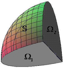
Ω = { ( x , y , z ) : x 2 + y 2 + z 2 < R 2 , x > 0 , y > 0 , − R < z < R } Ω conditional-set 𝑥 𝑦 𝑧 formulae-sequence superscript 𝑥 2 superscript 𝑦 2 superscript 𝑧 2 superscript 𝑅 2 formulae-sequence 𝑥 0 formulae-sequence 𝑦 0 𝑅 𝑧 𝑅 \Omega=\left\{(x,y,z):x^{2}+y^{2}+z^{2}<R^{2},\,x>0,y>0,-R<z<R\right\}
which is a quarter of a ball.
Figure 1: Domain Ω Ω \Omega
Problem D-N. Find a function u ( x , y , z ) ∈ C ( Ω ¯ ) ∩ C 2 ( Ω ) 𝑢 𝑥 𝑦 𝑧 𝐶 ¯ Ω superscript 𝐶 2 Ω u\left(x,y,z\right)\in C\left(\overline{\Omega}\right)\cap{C^{2}}\left(\Omega\right) satisfying Eq.(1) in Ω Ω \Omega
u ( x , y , z ) | x = 0 = τ 1 ( y , z ) , ( y , z ) ∈ Ω 1 ¯ , formulae-sequence evaluated-at 𝑢 𝑥 𝑦 𝑧 𝑥 0 subscript 𝜏 1 𝑦 𝑧 𝑦 𝑧 ¯ subscript Ω 1 u\left(x,y,z\right)|_{x=0}={\tau_{1}}\left(y,z\right),\,\left(y,z\right)\in\overline{\Omega_{1}}, ( 2 ) 2
y 2 β u ( x , y , z ) | y = 0 = ν 2 ( x , z ) , ( x , z ) ∈ Ω 2 , formulae-sequence evaluated-at superscript 𝑦 2 𝛽 𝑢 𝑥 𝑦 𝑧 𝑦 0 subscript 𝜈 2 𝑥 𝑧 𝑥 𝑧 subscript Ω 2 y^{2\beta}u\left(x,y,z\right)|_{y=0}=\nu_{2}\left(x,z\right),\,\,\,\left(x,z\right)\in\Omega_{2}, ( 3 ) 3
u ( x , y , z ) = φ ( x , y , z ) , ( x , y , z ) ∈ 𝕊 ¯ . formulae-sequence 𝑢 𝑥 𝑦 𝑧 𝜑 𝑥 𝑦 𝑧 𝑥 𝑦 𝑧 ¯ 𝕊 u\left(x,y,z\right)=\varphi\left(x,y,z\right),\,\,\,\left(x,y,z\right)\in\overline{\mathbb{S}}. ( 4 ) 4
Here
Ω 1 = { ( x , y , z ) : y 2 + z 2 < R 2 , x = 0 , y > 0 , − R < z < R } , Ω 2 = { ( x , y , z ) : x 2 + z 2 < R 2 , x > 0 , y = 0 , − R < z < R } , 𝕊 = { ( x , y , z ) : x 2 + y 2 + z 2 = R 2 , x > 0 , y > 0 , − R < z < R } , subscript Ω 1 conditional-set 𝑥 𝑦 𝑧 formulae-sequence superscript 𝑦 2 superscript 𝑧 2 superscript 𝑅 2 formulae-sequence 𝑥 0 formulae-sequence 𝑦 0 𝑅 𝑧 𝑅 subscript Ω 2 conditional-set 𝑥 𝑦 𝑧 formulae-sequence superscript 𝑥 2 superscript 𝑧 2 superscript 𝑅 2 formulae-sequence 𝑥 0 formulae-sequence 𝑦 0 𝑅 𝑧 𝑅 𝕊 conditional-set 𝑥 𝑦 𝑧 formulae-sequence superscript 𝑥 2 superscript 𝑦 2 superscript 𝑧 2 superscript 𝑅 2 formulae-sequence 𝑥 0 formulae-sequence 𝑦 0 𝑅 𝑧 𝑅 \begin{array}[]{l}\Omega_{1}=\left\{(x,y,z):y^{2}+z^{2}<R^{2},\,x=0,y>0,-R<z<R\right\},\hfill\\
\Omega_{2}=\left\{(x,y,z):x^{2}+z^{2}<R^{2},\,x>0,y=0,-R<z<R\right\},\hfill\\
\mathbb{S}=\left\{(x,y,z):x^{2}+y^{2}+z^{2}=R^{2},\,x>0,y>0,-R<z<R\right\},\hfill\\
\end{array}
τ 1 ( y , z ) , ν 2 ( x , z ) , φ ( x , y , z ) subscript 𝜏 1 𝑦 𝑧 subscript 𝜈 2 𝑥 𝑧 𝜑 𝑥 𝑦 𝑧
{\tau_{1}}\left(y,z\right),{\nu_{2}}\left(x,z\right),\varphi\left(x,y,z\right) τ 1 ( y , z ) | Υ 1 = φ ( x , y , z ) | Υ 1 , evaluated-at subscript 𝜏 1 𝑦 𝑧 subscript Υ 1 evaluated-at 𝜑 𝑥 𝑦 𝑧 subscript Υ 1 \left.{\tau_{1}\left(y,z\right)}\right|_{\Upsilon_{1}}=\left.{\varphi\left(x,y,z\right)}\right|_{\Upsilon_{1}}, ( Υ 1 := y 2 + z 2 = R 2 ) assign subscript Υ 1 superscript 𝑦 2 superscript 𝑧 2 superscript 𝑅 2 \left(\Upsilon_{1}:=y^{2}+z^{2}=R^{2}\right)
Remark. The uniqueness of solution of the problem D-N can be proved using classical ”a-b-c” method as in the work [20] or using extremume principle for elliptic equations [8]. We note also that the uniqueness theorem can be proved for more general domains.
First we give a definition of the Green’s function of the problem D-N.
Definition. We call the function G ( M , M 0 ) 𝐺 𝑀 subscript 𝑀 0 G\left(M,M_{0}\right)
1.
it satisfies equation
G x x + G y y + G z z + 2 α x u x + 2 β y u y = − δ ( M , M 0 ) subscript 𝐺 𝑥 𝑥 subscript 𝐺 𝑦 𝑦 subscript 𝐺 𝑧 𝑧 2 𝛼 𝑥 subscript 𝑢 𝑥 2 𝛽 𝑦 subscript 𝑢 𝑦 𝛿 𝑀 subscript 𝑀 0 G_{xx}+G_{yy}+G_{zz}+\frac{2\alpha}{x}u_{x}+\frac{2\beta}{y}u_{y}=-\delta\left(M,M_{0}\right)
in Ω Ω \Omega
2.
it satisfies boundary conditions
G | x = 0 = 0 , y 2 β G y | y = 0 = 0 , G | 𝕊 ¯ = 0 ; formulae-sequence evaluated-at 𝐺 𝑥 0 0 formulae-sequence evaluated-at superscript 𝑦 2 𝛽 subscript 𝐺 𝑦 𝑦 0 0 evaluated-at 𝐺 ¯ 𝕊 0 \left.G\right|_{x=0}=0,\,\,y^{2\beta}\left.G_{y}\right|_{y=0}=0,\,\,\left.G\right|_{\overline{\mathbb{S}}}=0;
3.
it can be represented as
G ( M , M 0 ) = q ( M , M 0 ) + q ∗ ( M , M 0 ¯ ) . 𝐺 𝑀 subscript 𝑀 0 𝑞 𝑀 subscript 𝑀 0 superscript 𝑞 𝑀 ¯ subscript 𝑀 0 G\left(M,M_{0}\right)=q\left(M,M_{0}\right)+q^{*}\left(M,\overline{M_{0}}\right). ( 5 ) 5
Here δ 𝛿 \delta M ( x , y , z ) 𝑀 𝑥 𝑦 𝑧 M(x,y,z) M 0 ( x , y , z ) subscript 𝑀 0 𝑥 𝑦 𝑧 M_{0}(x,y,z) Ω Ω \Omega M 0 ¯ ( x 0 ¯ , z 0 ¯ , z 0 ¯ ) ¯ subscript 𝑀 0 ¯ subscript 𝑥 0 ¯ subscript 𝑧 0 ¯ subscript 𝑧 0 \overline{M_{0}}\left(\overline{x_{0}},\overline{z_{0}},\overline{z_{0}}\right) M 0 subscript 𝑀 0 M_{0}
x 0 ¯ = − R 2 R 0 2 x 0 , y 0 ¯ = − R 2 R 0 2 y 0 , z 0 ¯ = − R 2 R 0 2 z 0 , R 0 2 = x 0 2 + y 0 2 + z 0 2 , formulae-sequence ¯ subscript 𝑥 0 superscript 𝑅 2 superscript subscript 𝑅 0 2 subscript 𝑥 0 formulae-sequence ¯ subscript 𝑦 0 superscript 𝑅 2 superscript subscript 𝑅 0 2 subscript 𝑦 0 formulae-sequence ¯ subscript 𝑧 0 superscript 𝑅 2 superscript subscript 𝑅 0 2 subscript 𝑧 0 superscript subscript 𝑅 0 2 superscript subscript 𝑥 0 2 superscript subscript 𝑦 0 2 superscript subscript 𝑧 0 2 \overline{x_{0}}=-\frac{R^{2}}{R_{0}^{2}}x_{0},\,\,\overline{y_{0}}=-\frac{R^{2}}{R_{0}^{2}}y_{0},\,\,\overline{z_{0}}=-\frac{R^{2}}{R_{0}^{2}}z_{0},\,\,R_{0}^{2}=x_{0}^{2}+y_{0}^{2}+z_{0}^{2},
q ( M , M 0 ) = k ( r 2 ) α − β − 3 2 ( x x 0 ) 1 − 2 α F 2 ( 3 2 − α + β , 1 − α , β ; 2 − 2 α , 2 β ; ξ , η ) 𝑞 𝑀 subscript 𝑀 0 𝑘 superscript superscript 𝑟 2 𝛼 𝛽 3 2 superscript 𝑥 subscript 𝑥 0 1 2 𝛼 subscript 𝐹 2 3 2 𝛼 𝛽 1 𝛼 𝛽 2 2 𝛼 2 𝛽 𝜉 𝜂 q\left(M,M_{0}\right)=k\left(r^{2}\right)^{\alpha-\beta-\frac{3}{2}}\left(xx_{0}\right)^{1-2\alpha}F_{2}\left(\frac{3}{2}-\alpha+\beta,1-\alpha,\beta;2-2\alpha,2\beta;\xi,\eta\right) ( 6 ) 6
is one of the fundamental solutions of Eq.(1) [20],
F 2 ( a ; b 1 , b 2 ; c 1 , c 2 ; x , y ) = ∑ i , j = 0 ∞ ( a ) i + j ( b 1 ) i ( b 2 ) j ( c 1 ) i ( c 2 ) j i ! j ! x i y j subscript 𝐹 2 𝑎 subscript 𝑏 1 subscript 𝑏 2 subscript 𝑐 1 subscript 𝑐 2 𝑥 𝑦
superscript subscript 𝑖 𝑗
0 subscript 𝑎 𝑖 𝑗 subscript subscript 𝑏 1 𝑖 subscript subscript 𝑏 2 𝑗 subscript subscript 𝑐 1 𝑖 subscript subscript 𝑐 2 𝑗 𝑖 𝑗 superscript 𝑥 𝑖 superscript 𝑦 𝑗 {F_{2}}\left({a;{b_{1}},{b_{2}};{c_{1}},{c_{2}};x,y}\right)=\sum\limits_{i,j=0}^{\infty}{\frac{{{{\left(a\right)}_{i+j}}{{\left({{b_{1}}}\right)}_{i}}{{\left({{b_{2}}}\right)}_{j}}}}{{{{\left({{c_{1}}}\right)}_{i}}{{\left({{c_{2}}}\right)}_{j}}i!j!}}{x^{i}}{y^{j}}}
is Appel’s hypergeometric function [21],
q ∗ ( M , M 0 ) = − ( R R 0 ) 3 − 2 α + 2 β q ( M , M ¯ 0 ) superscript 𝑞 𝑀 subscript 𝑀 0 superscript 𝑅 subscript 𝑅 0 3 2 𝛼 2 𝛽 𝑞 𝑀 subscript ¯ 𝑀 0 q^{*}\left(M,M_{0}\right)=-\left(\frac{R}{R_{0}}\right)^{3-2\alpha+2\beta}q\left(M,\overline{M}_{0}\right)
is a regular part of the Green’s function (5), i.e. satisfies Eq.(1) in any point of Ω Ω \Omega
ξ = 1 − r 1 2 r 2 , η = 1 − r 2 2 r 2 , r 2 = ( x − x 0 ) 2 + ( y − y 0 ) 2 + ( z − z 0 ) 2 , formulae-sequence 𝜉 1 superscript subscript 𝑟 1 2 superscript 𝑟 2 formulae-sequence 𝜂 1 superscript subscript 𝑟 2 2 superscript 𝑟 2 superscript 𝑟 2 superscript 𝑥 subscript 𝑥 0 2 superscript 𝑦 subscript 𝑦 0 2 superscript 𝑧 subscript 𝑧 0 2 \xi=1-\frac{r_{1}^{2}}{r^{2}},\,\,\eta=1-\frac{r_{2}^{2}}{r^{2}},\,\,r^{2}=(x-x_{0})^{2}+(y-y_{0})^{2}+(z-z_{0})^{2},
r 1 2 = ( x + x 0 ) 2 + ( y − y 0 ) 2 + ( z − z 0 ) 2 , r 2 2 = ( x − x 0 ) 2 + ( y + y 0 ) 2 + ( z − z 0 ) 2 , formulae-sequence superscript subscript 𝑟 1 2 superscript 𝑥 subscript 𝑥 0 2 superscript 𝑦 subscript 𝑦 0 2 superscript 𝑧 subscript 𝑧 0 2 superscript subscript 𝑟 2 2 superscript 𝑥 subscript 𝑥 0 2 superscript 𝑦 subscript 𝑦 0 2 superscript 𝑧 subscript 𝑧 0 2 r_{1}^{2}=(x+x_{0})^{2}+(y-y_{0})^{2}+(z-z_{0})^{2},\,\,r_{2}^{2}=(x-x_{0})^{2}+(y+y_{0})^{2}+(z-z_{0})^{2},
k = 1 2 π Γ ( 1 − α ) Γ ( β ) Γ ( 2 − 2 α + 2 β ) Γ ( 2 − 2 α ) Γ ( 2 β ) Γ ( 1 − α + β ) . 𝑘 1 2 𝜋 Γ 1 𝛼 Γ 𝛽 Γ 2 2 𝛼 2 𝛽 Γ 2 2 𝛼 Γ 2 𝛽 Γ 1 𝛼 𝛽 k=\frac{1}{2\pi}\frac{\Gamma(1-\alpha)\Gamma(\beta)\Gamma(2-2\alpha+2\beta)}{\Gamma(2-2\alpha)\Gamma(2\beta)\Gamma(1-\alpha+\beta)}. ( 7 ) 7
Excise from the domain Ω Ω \Omega M 0 subscript 𝑀 0 M_{0} ρ > 0 𝜌 0 \rho>0 C ρ subscript 𝐶 𝜌 C_{\rho} Ω ρ subscript Ω 𝜌 \Omega_{\rho} Ω Ω \Omega
Applying Green’s formula [22] in this domain, one can obtain the following:
∬ C ρ x 2 α y 2 β [ u ∂ G ∂ n − G ∂ u ∂ n ] 𝑑 s = ∬ Ω 1 y 2 β τ 1 ( y , z ) G ∗ ( M , M 0 ) 𝑑 y 𝑑 z + ∬ Ω 2 x 2 α ν 2 ( x , z ) G ∗ ∗ ( M , M 0 ) 𝑑 x 𝑑 z + ∬ 𝕊 x 2 α y 2 β φ ( σ ) ∂ G ∂ n 𝑑 σ . subscript double-integral subscript 𝐶 𝜌 superscript 𝑥 2 𝛼 superscript 𝑦 2 𝛽 delimited-[] 𝑢 𝐺 𝑛 𝐺 𝑢 𝑛 differential-d 𝑠 subscript double-integral subscript Ω 1 superscript 𝑦 2 𝛽 subscript 𝜏 1 𝑦 𝑧 superscript 𝐺 𝑀 subscript 𝑀 0 differential-d 𝑦 differential-d 𝑧 subscript double-integral subscript Ω 2 superscript 𝑥 2 𝛼 subscript 𝜈 2 𝑥 𝑧 superscript 𝐺 absent 𝑀 subscript 𝑀 0 differential-d 𝑥 differential-d 𝑧 subscript double-integral 𝕊 superscript 𝑥 2 𝛼 superscript 𝑦 2 𝛽 𝜑 𝜎 𝐺 𝑛 differential-d 𝜎 \begin{array}[]{l}\iint\limits_{C_{\rho}}{x^{2\alpha}y^{2\beta}\left[\displaystyle{u\frac{\partial G}{\partial n}-G\frac{\partial u}{\partial n}}\right]ds}=\iint\limits_{\Omega_{1}}y^{2\beta}\tau_{1}(y,z)G^{*}\left(M,M_{0}\right)dydz\hfill\\
+\iint\limits_{\Omega_{2}}x^{2\alpha}\nu_{2}(x,z)G^{**}\left(M,M_{0}\right)dxdz+\iint\limits_{\mathbb{S}}x^{2\alpha}y^{2\beta}\varphi(\sigma)\displaystyle{\frac{\partial G}{\partial n}}d\sigma.\hfill\\
\end{array} ( 8 ) 8
Here G ∗ ( M , M 0 ) = x 2 β ∂ G ( M , M 0 ) ∂ x | x = 0 superscript 𝐺 𝑀 subscript 𝑀 0 evaluated-at superscript 𝑥 2 𝛽 𝐺 𝑀 subscript 𝑀 0 𝑥 𝑥 0 G^{*}\left(M,M_{0}\right)=\left.x^{2\beta}\displaystyle{\frac{\partial G\left(M,M_{0}\right)}{\partial x}}\right|_{x=0} G ∗ ∗ ( M , M 0 ) = G ( M , M 0 ) | y = 0 superscript 𝐺 absent 𝑀 subscript 𝑀 0 evaluated-at 𝐺 𝑀 subscript 𝑀 0 𝑦 0 G^{**}\left(M,M_{0}\right)=\left.G\left(M,M_{0}\right)\right|_{y=0} n 𝑛 n ∂ Ω Ω \partial\Omega
Let us first evaluate an integral
I = ∬ C ρ x 2 α y 2 β u ∂ G ∂ n 𝑑 s . 𝐼 subscript double-integral subscript 𝐶 𝜌 superscript 𝑥 2 𝛼 superscript 𝑦 2 𝛽 𝑢 𝐺 𝑛 differential-d 𝑠 I=\iint\limits_{C_{\rho}}x^{2\alpha}y^{2\beta}u\frac{\partial G}{\partial n}ds. ( 9 ) 9
Based on (5) we write (9) as follows:
I = I 1 + I 2 = ∬ C ρ x 2 α y 2 β u ∂ q ∂ n 𝑑 s + ∬ C ρ x 2 α y 2 β u ∂ q ∗ ∂ n 𝑑 s , 𝐼 subscript 𝐼 1 subscript 𝐼 2 subscript double-integral subscript 𝐶 𝜌 superscript 𝑥 2 𝛼 superscript 𝑦 2 𝛽 𝑢 𝑞 𝑛 differential-d 𝑠 subscript double-integral subscript 𝐶 𝜌 superscript 𝑥 2 𝛼 superscript 𝑦 2 𝛽 𝑢 superscript 𝑞 𝑛 differential-d 𝑠 I=I_{1}+I_{2}=\iint\limits_{C_{\rho}}x^{2\alpha}y^{2\beta}u\frac{\partial q}{\partial n}ds+\iint\limits_{C_{\rho}}x^{2\alpha}y^{2\beta}u\frac{\partial q^{*}}{\partial n}ds,
where
∂ q ∂ n = ∂ q ∂ x cos ( n , x ) + ∂ q ∂ y cos ( n , y ) + ∂ q ∂ z cos ( n , z ) . 𝑞 𝑛 𝑞 𝑥 𝑛 𝑥 𝑞 𝑦 𝑛 𝑦 𝑞 𝑧 𝑛 𝑧 \frac{\partial q}{\partial n}=\frac{\partial q}{\partial x}\cos(n,x)+\frac{\partial q}{\partial y}\cos(n,y)+\frac{\partial q}{\partial z}\cos(n,z). ( 10 ) 10
Formal calculation gives
∂ q ∂ x = ∂ ∂ x [ k P 1 P 2 F 2 ( … ) ] = k [ ( ∂ P 1 ∂ x P 2 + P 1 ∂ P 2 ∂ x ) F 2 ( … ) + P 1 P 2 ( ∂ F 2 ∂ ξ ξ x + ∂ F 2 ∂ η η x ) ] , 𝑞 𝑥 𝑥 delimited-[] 𝑘 subscript 𝑃 1 subscript 𝑃 2 subscript 𝐹 2 … absent 𝑘 delimited-[] subscript 𝑃 1 𝑥 subscript 𝑃 2 subscript 𝑃 1 subscript 𝑃 2 𝑥 subscript 𝐹 2 … subscript 𝑃 1 subscript 𝑃 2 subscript 𝐹 2 𝜉 subscript 𝜉 𝑥 subscript 𝐹 2 𝜂 subscript 𝜂 𝑥 \begin{array}[]{l}\displaystyle{\frac{\partial q}{\partial x}=\frac{\partial}{\partial x}\left[kP_{1}P_{2}F_{2}(...)\right]\hfill}\\
\displaystyle{=k\left[\left(\frac{\partial P_{1}}{\partial x}P_{2}+P_{1}\frac{\partial P_{2}}{\partial x}\right)F_{2}(...)+P_{1}P_{2}\left(\frac{\partial F_{2}}{\partial\xi}\xi_{x}+\frac{\partial F_{2}}{\partial\eta}\eta_{x}\right)\right]},\hfill\\
\end{array}
where P 1 = ( r 2 ) α − β − 3 2 , P 2 = ( x x 0 ) 1 − 2 α formulae-sequence subscript 𝑃 1 superscript superscript 𝑟 2 𝛼 𝛽 3 2 subscript 𝑃 2 superscript 𝑥 subscript 𝑥 0 1 2 𝛼 P_{1}=\left(r^{2}\right)^{\alpha-\beta-\frac{3}{2}},\,\,P_{2}=\left(xx_{0}\right)^{1-2\alpha}
Using formula of differentiation for hypergeometric function F 2 ( … ) subscript 𝐹 2 … F_{2}(...)
∂ i + j F 2 ( a , b 1 , b 2 ; c 1 , c 2 ; x , y ) ∂ x i y j = ( a ) i + j ( b 1 ) i ( b 2 ) j ( c 1 ) i ( c 2 ) j F 2 ( a + i + j , b 1 + i , b 2 + j ; c 1 + i , c 2 + j ; x , y ) superscript 𝑖 𝑗 subscript 𝐹 2 𝑎 subscript 𝑏 1 subscript 𝑏 2 subscript 𝑐 1 subscript 𝑐 2 𝑥 𝑦 superscript 𝑥 𝑖 superscript 𝑦 𝑗 absent subscript 𝑎 𝑖 𝑗 subscript subscript 𝑏 1 𝑖 subscript subscript 𝑏 2 𝑗 subscript subscript 𝑐 1 𝑖 subscript subscript 𝑐 2 𝑗 subscript 𝐹 2 𝑎 𝑖 𝑗 subscript 𝑏 1 𝑖 subscript 𝑏 2 𝑗 subscript 𝑐 1 𝑖 subscript 𝑐 2 𝑗 𝑥 𝑦 \begin{array}[]{l}\displaystyle{\frac{\partial^{i+j}F_{2}\left(a,b_{1},b_{2};c_{1},c_{2};x,y\right)}{\partial x^{i}y^{j}}}=\hfill\\
\displaystyle{\frac{\left(a\right)_{i+j}\left(b_{1}\right)_{i}\left(b_{2}\right)_{j}}{\left(c_{1}\right)_{i}\left(c_{2}\right)_{j}}F_{2}\left(a+i+j,b_{1}+i,b_{2}+j;c_{1}+i,c_{2}+j;x,y\right)\hfill}\\
\end{array}
we get
∂ ∂ ξ F 2 ( 3 2 − α + β , 1 − α , β ; 2 − 2 α , 2 β ; ξ , η ) = ( 3 2 − α + β ) ( 1 − α ) ( 2 − 2 α ) F 2 ( 5 2 − α + β , 2 − α , β ; 3 − 2 α , 2 β ; ξ , η ) , 𝜉 subscript 𝐹 2 3 2 𝛼 𝛽 1 𝛼 𝛽 2 2 𝛼 2 𝛽 𝜉 𝜂 absent 3 2 𝛼 𝛽 1 𝛼 2 2 𝛼 subscript 𝐹 2 5 2 𝛼 𝛽 2 𝛼 𝛽 3 2 𝛼 2 𝛽 𝜉 𝜂 \begin{array}[]{l}\displaystyle{\frac{\partial}{\partial\xi}F_{2}\left(\frac{3}{2}-\alpha+\beta,1-\alpha,\beta;2-2\alpha,2\beta;\xi,\eta\right)\hfill}\\
\displaystyle{=\frac{\left(\frac{3}{2}-\alpha+\beta\right)\left(1-\alpha\right)}{\left(2-2\alpha\right)}F_{2}\left(\frac{5}{2}-\alpha+\beta,2-\alpha,\beta;3-2\alpha,2\beta;\xi,\eta\right)},\hfill\\
\end{array}
∂ ∂ η F 2 ( 3 2 − α + β , 1 − α , β ; 2 − 2 α , 2 β ; ξ , η ) = ( 3 2 − α + β ) β 2 β F 2 ( 5 2 − α + β , 1 − α , β + 1 ; 2 − 2 α , 2 β + 1 ; ξ , η ) . 𝜂 subscript 𝐹 2 3 2 𝛼 𝛽 1 𝛼 𝛽 2 2 𝛼 2 𝛽 𝜉 𝜂 absent 3 2 𝛼 𝛽 𝛽 2 𝛽 subscript 𝐹 2 5 2 𝛼 𝛽 1 𝛼 𝛽 1 2 2 𝛼 2 𝛽 1 𝜉 𝜂 \begin{array}[]{l}\displaystyle{\frac{\partial}{\partial\eta}F_{2}\left(\frac{3}{2}-\alpha+\beta,1-\alpha,\beta;2-2\alpha,2\beta;\xi,\eta\right)\hfill}\\
\displaystyle{=\frac{\left(\frac{3}{2}-\alpha+\beta\right)\beta}{2\beta}F_{2}\left(\frac{5}{2}-\alpha+\beta,1-\alpha,\beta+1;2-2\alpha,2\beta+1;\xi,\eta\right).\hfill}\\
\end{array}
Considering
∂ P 1 ∂ x = 2 ( x − x 0 ) r 2 ( α − β − 3 2 ) P 1 , ∂ P 2 ∂ x = 1 − 2 α x P 2 , formulae-sequence subscript 𝑃 1 𝑥 2 𝑥 subscript 𝑥 0 superscript 𝑟 2 𝛼 𝛽 3 2 subscript 𝑃 1 subscript 𝑃 2 𝑥 1 2 𝛼 𝑥 subscript 𝑃 2 \frac{\partial P_{1}}{\partial x}=\frac{2\left(x-x_{0}\right)}{r^{2}}\left(\alpha-\beta-\frac{3}{2}\right)P_{1},\,\,\frac{\partial P_{2}}{\partial x}=\frac{1-2\alpha}{x}P_{2},
ξ x = − 4 x 0 r 2 − 2 ( x − x 0 ) r 2 ξ , η x = − 2 ( x − x 0 ) r 2 η , formulae-sequence subscript 𝜉 𝑥 4 subscript 𝑥 0 superscript 𝑟 2 2 𝑥 subscript 𝑥 0 superscript 𝑟 2 𝜉 subscript 𝜂 𝑥 2 𝑥 subscript 𝑥 0 superscript 𝑟 2 𝜂 \xi_{x}=-\frac{4x_{0}}{r^{2}}-\frac{2\left(x-x_{0}\right)}{r^{2}}\xi,\,\eta_{x}=-\frac{2\left(x-x_{0}\right)}{r^{2}}\eta,
we have
∂ q ∂ x = k P 1 P 2 r 2 [ 2 ( x − x 0 ) ( α − β − 3 2 ) × F 2 ( 3 2 − α + β , 1 − α , β ; 2 − 2 α , 2 β ; ξ , η ) + 1 − 2 α x r 2 × F 2 ( 3 2 − α + β , 1 − α , β ; 2 − 2 α , 2 β ; ξ , η ) − 2 x 0 ( 3 2 − α + β ) × F 2 ( 5 2 − α + β , 2 − α , β ; 3 − 2 α , 2 β ; ξ , η ) − 2 ( x − x 0 ) ( 3 2 − α + β ) ξ 1 − α 2 − 2 α × F 2 ( 5 2 − α + β , 2 − α , β ; 3 − 2 α , 2 β ; ξ , η ) − 2 ( x − x 0 ) ( 3 2 − α + β ) η β 2 β × F 2 ( 5 2 − α + β , 1 − α , β + 1 ; 2 − 2 α , 2 β + 1 ; ξ , η ) ] . \begin{array}[]{l}\displaystyle{\frac{\partial q}{\partial x}=\frac{kP_{1}P_{2}}{r^{2}}\left[2\left(x-x_{0}\right)\left(\alpha-\beta-\frac{3}{2}\right)\right.\hfill}\\
\displaystyle{\times F_{2}\left(\frac{3}{2}-\alpha+\beta,1-\alpha,\beta;2-2\alpha,2\beta;\xi,\eta\right)+\frac{1-2\alpha}{x}r^{2}\hfill}\\
\displaystyle{\times F_{2}\left(\frac{3}{2}-\alpha+\beta,1-\alpha,\beta;2-2\alpha,2\beta;\xi,\eta\right)-2x_{0}\left(\frac{3}{2}-\alpha+\beta\right)\hfill}\\
\displaystyle{\times F_{2}\left(\frac{5}{2}-\alpha+\beta,2-\alpha,\beta;3-2\alpha,2\beta;\xi,\eta\right)-2\left(x-x_{0}\right)\left(\frac{3}{2}-\alpha+\beta\right)\xi\frac{1-\alpha}{2-2\alpha}\hfill}\\
\displaystyle{\times F_{2}\left(\frac{5}{2}-\alpha+\beta,2-\alpha,\beta;3-2\alpha,2\beta;\xi,\eta\right)-2\left(x-x_{0}\right)\left(\frac{3}{2}-\alpha+\beta\right)\eta\frac{\beta}{2\beta}\hfill}\\
\displaystyle{\left.\times F_{2}\left(\frac{5}{2}-\alpha+\beta,1-\alpha,\beta+1;2-2\alpha,2\beta+1;\xi,\eta\right)\right]}.\hfill\\
\end{array} ( 11 ) 11
Now we apply to (11) the following adjacent relation [21]
x b 1 c 1 F 2 ( a + 1 , b 1 + 1 , b 2 ; c 1 + 1 , c 2 ; x , y ) + y b 2 c 2 F 2 ( a + 1 , b 1 , b 2 + 1 ; c 1 , c 2 + 1 ; x , y ) = F 2 ( a + 1 , b 1 , b 2 ; c 1 , c 2 ; x , y ) − F 2 ( a , b 1 , b 2 ; c 1 , c 2 ; x , y ) 𝑥 subscript 𝑏 1 subscript 𝑐 1 subscript 𝐹 2 𝑎 1 subscript 𝑏 1 1 subscript 𝑏 2 subscript 𝑐 1 1 subscript 𝑐 2 𝑥 𝑦 𝑦 subscript 𝑏 2 subscript 𝑐 2 subscript 𝐹 2 𝑎 1 subscript 𝑏 1 subscript 𝑏 2 1 subscript 𝑐 1 subscript 𝑐 2 1 𝑥 𝑦 absent subscript 𝐹 2 𝑎 1 subscript 𝑏 1 subscript 𝑏 2 subscript 𝑐 1 subscript 𝑐 2 𝑥 𝑦 subscript 𝐹 2 𝑎 subscript 𝑏 1 subscript 𝑏 2 subscript 𝑐 1 subscript 𝑐 2 𝑥 𝑦 \begin{array}[]{l}\displaystyle{x\frac{b_{1}}{c_{1}}F_{2}\left(a+1,b_{1}+1,b_{2};c_{1}+1,c_{2};x,y\right)\hfill}\\
\displaystyle{+y\frac{b_{2}}{c_{2}}F_{2}\left(a+1,b_{1},b_{2}+1;c_{1},c_{2}+1;x,y\right)\hfill}\\
\displaystyle{=F_{2}\left(a+1,b_{1},b_{2};c_{1},c_{2};x,y\right)-F_{2}\left(a,b_{1},b_{2};c_{1},c_{2};x,y\right)\hfill}\\
\end{array}
and will obtain
∂ q ∂ x = k P 1 P 2 r 2 [ 2 ( x − x 0 ) ( α − β − 3 2 ) × F 2 ( 5 2 − α + β , 1 − α , β ; 2 − 2 α , 2 β ; ξ , η ) + 2 x 0 ( α − β − 3 2 ) F 2 ( 5 2 − α + β , 2 − α , β ; 3 − 2 α , 2 β ; ξ , η ) ] + k P 1 P 2 1 − 2 α x r 2 F 2 ( 3 2 − α + β , 1 − α , β ; 2 − 2 α , 2 β ; ξ , η ) . \begin{array}[]{l}\displaystyle{\frac{\partial q}{\partial x}=\frac{kP_{1}P_{2}}{r^{2}}\left[2\left(x-x_{0}\right)\left(\alpha-\beta-\frac{3}{2}\right)\right.\hfill}\\
\displaystyle{\times F_{2}\left(\frac{5}{2}-\alpha+\beta,1-\alpha,\beta;2-2\alpha,2\beta;\xi,\eta\right)\hfill}\\
\displaystyle{\left.+2x_{0}\left(\alpha-\beta-\frac{3}{2}\right)F_{2}\left(\frac{5}{2}-\alpha+\beta,2-\alpha,\beta;3-2\alpha,2\beta;\xi,\eta\right)\right]\hfill}\\
\displaystyle{+kP_{1}P_{2}\frac{1-2\alpha}{x}r^{2}F_{2}\left(\frac{3}{2}-\alpha+\beta,1-\alpha,\beta;2-2\alpha,2\beta;\xi,\eta\right)}.\hfill\\
\end{array} ( 12 ) 12
Similarly we get
∂ q ∂ y = k P 1 P 2 r 2 [ 2 ( y − y 0 ) ( α − β − 3 2 ) × F 2 ( 5 2 − α + β , 1 − α , β ; 2 − 2 α , 2 β ; ξ , η ) + 2 y 0 ( α − β − 3 2 ) F 2 ( 5 2 − α + β , 1 − α , β + 1 ; 2 − 2 α , 2 β + 1 ; ξ , η ) ] , \begin{array}[]{l}\displaystyle{\frac{\partial q}{\partial y}=\frac{kP_{1}P_{2}}{r^{2}}\left[2\left(y-y_{0}\right)\left(\alpha-\beta-\frac{3}{2}\right)\right.\hfill}\\
\displaystyle{\times F_{2}\left(\frac{5}{2}-\alpha+\beta,1-\alpha,\beta;2-2\alpha,2\beta;\xi,\eta\right)\hfill}\\
\displaystyle{\left.+2y_{0}\left(\alpha-\beta-\frac{3}{2}\right)F_{2}\left(\frac{5}{2}-\alpha+\beta,1-\alpha,\beta+1;2-2\alpha,2\beta+1;\xi,\eta\right)\right]},\hfill\\
\end{array} ( 13 ) 13
∂ q ∂ z = k P 1 P 2 r 2 2 ( z − z 0 ) ( α − β − 3 2 ) F 2 ( 5 2 − α + β , 1 − α , β ; 2 − 2 α , 2 β ; ξ , η ) . 𝑞 𝑧 𝑘 subscript 𝑃 1 subscript 𝑃 2 superscript 𝑟 2 2 𝑧 subscript 𝑧 0 𝛼 𝛽 3 2 subscript 𝐹 2 5 2 𝛼 𝛽 1 𝛼 𝛽 2 2 𝛼 2 𝛽 𝜉 𝜂 \frac{\partial q}{\partial z}=\frac{kP_{1}P_{2}}{r^{2}}2\left(z-z_{0}\right)\left(\alpha-\beta-\frac{3}{2}\right)F_{2}\left(\frac{5}{2}-\alpha+\beta,1-\alpha,\beta;2-2\alpha,2\beta;\xi,\eta\right). ( 14 ) 14
Taking (12)-(14) into account, from (10) we get the following:
∂ ∂ n q ( M , M 0 ) = ( α − β − 3 2 ) k P 1 P 2 × F 2 ( 5 2 − α + β , 1 − α , β ; 2 − 2 α , 2 β ; ξ , η ) ∂ ∂ n [ ln r 2 ] + k P 1 P 2 r 2 ( α − β − 3 2 ) × [ 2 x 0 F 2 ( 5 2 − α + β , 2 − α , β ; 3 − 2 α , 2 β ; ξ , η ) + 2 y 0 F 2 ( 5 2 − α + β , 1 − α , β + 1 ; 2 − 2 α , 2 β + 1 ; ξ , η ) ] + k P 1 P 2 1 − 2 α x F 2 ( 3 2 − α + β , 1 − α , β ; 2 − 2 α , 2 β ; ξ , η ) . \begin{array}[]{l}\displaystyle{\frac{\partial}{\partial n}q\left(M,M_{0}\right)=\left(\alpha-\beta-\frac{3}{2}\right)kP_{1}P_{2}\hfill}\\
\displaystyle{\times F_{2}\left(\frac{5}{2}-\alpha+\beta,1-\alpha,\beta;2-2\alpha,2\beta;\xi,\eta\right)\frac{\partial}{\partial n}\left[\ln{r^{2}}\right]+\frac{kP_{1}P_{2}}{r^{2}}\left(\alpha-\beta-\frac{3}{2}\right)\hfill}\\
\displaystyle{\times\left[2x_{0}F_{2}\left(\frac{5}{2}-\alpha+\beta,2-\alpha,\beta;3-2\alpha,2\beta;\xi,\eta\right)\right.\hfill}\\
\displaystyle{\left.+2y_{0}F_{2}\left(\frac{5}{2}-\alpha+\beta,1-\alpha,\beta+1;2-2\alpha,2\beta+1;\xi,\eta\right)\right]\hfill}\\
\displaystyle{+kP_{1}P_{2}\frac{1-2\alpha}{x}F_{2}\left(\frac{3}{2}-\alpha+\beta,1-\alpha,\beta;2-2\alpha,2\beta;\xi,\eta\right).\hfill}\\
\end{array} ( 15 ) 15
Now consider the integral
I 1 = ∬ C ρ x 2 α y 2 β u ∂ q ∂ n 𝑑 S = I 11 + I 12 + I 13 = ∬ C ρ x 2 α y 2 β ( α − β − 3 2 ) k P 1 P 2 × F 2 ( 5 2 − α + β , 1 − α , β ; 2 − 2 α , 2 β ; ξ , η ) ∂ ∂ n [ ln r 2 ] u ( M 0 ) d s + ∬ C ρ x 2 α y 2 β k P 1 P 2 r 2 ( α − β − 3 2 ) × [ 2 x 0 F 2 ( 5 2 − α + β , 2 − α , β ; 3 − 2 α , 2 β ; ξ , η ) + 2 y 0 F 2 ( 5 2 − α + β , 1 − α , β + 1 ; 2 − 2 α , 2 β + 1 ; ξ , η ) ] u ( M 0 ) d s + ∬ C ρ x 2 α y 2 β k P 1 P 2 1 − 2 α x F 2 ( 3 2 − α + β , 1 − α , β ; 2 − 2 α , 2 β ; ξ , η ) u ( M 0 ) 𝑑 s . \begin{array}[]{l}\displaystyle{I_{1}=\iint\limits_{C_{\rho}}{x^{2\alpha}y^{2\beta}u\frac{\partial q}{\partial n}dS}=I_{11}+I_{12}+I_{13}\hfill}\\
\displaystyle{=\iint\limits_{C_{\rho}}{x^{2\alpha}y^{2\beta}\left(\alpha-\beta-\frac{3}{2}\right)kP_{1}P_{2}\hfill}}\\
\displaystyle{\times F_{2}\left(\frac{5}{2}-\alpha+\beta,1-\alpha,\beta;2-2\alpha,2\beta;\xi,\eta\right)\frac{\partial}{\partial n}\left[\ln{r^{2}}\right]u\left(M_{0}\right)ds\hfill}\\
\displaystyle{+\iint\limits_{C_{\rho}}{x^{2\alpha}y^{2\beta}\frac{kP_{1}P_{2}}{r}^{2}\left(\alpha-\beta-\frac{3}{2}\right)\hfill}}\\
\displaystyle{\times\left[2x_{0}F_{2}\left(\frac{5}{2}-\alpha+\beta,2-\alpha,\beta;3-2\alpha,2\beta;\xi,\eta\right)\right.\hfill}\\
\displaystyle{\left.+2y_{0}F_{2}\left(\frac{5}{2}-\alpha+\beta,1-\alpha,\beta+1;2-2\alpha,2\beta+1;\xi,\eta\right)\right]u\left(M_{0}\right)ds\hfill}\\
\displaystyle{+\iint\limits_{C_{\rho}}{x^{2\alpha}y^{2\beta}kP_{1}P_{2}\frac{1-2\alpha}{x}F_{2}\left(\frac{3}{2}-\alpha+\beta,1-\alpha,\beta;2-2\alpha,2\beta;\xi,\eta\right)u\left(M_{0}\right)ds}}.\hfill\\
\end{array}
We use the following spherical system of coordinates [22]:
x = x 0 + ρ sin θ cos ψ , y = y 0 + ρ sin θ sin ψ , z = z 0 + ρ cos θ , 0 < θ < π , 0 < ψ < 2 π , 0 < ρ < ∞ . formulae-sequence 𝑥 subscript 𝑥 0 𝜌 𝜃 𝜓 formulae-sequence 𝑦 subscript 𝑦 0 𝜌 𝜃 𝜓 𝑧 subscript 𝑧 0 𝜌 𝜃 formulae-sequence 0 𝜃 𝜋 0 𝜓 2 𝜋 0 𝜌 \begin{array}[]{l}x={x_{0}}+\rho\sin\theta\cos\psi,\,\,y={y_{0}}+\rho\sin\theta\sin\psi,\,\,z={z_{0}}+\rho\cos\theta,\hfill\\
0<\theta<\pi,\,0<\psi<2\pi,\,0<\rho<\infty.\hfill\\
\end{array}
Then we have
I 11 = − 2 ( α − β − 3 2 ) k ∫ 0 2 π 𝑑 ψ ∫ 0 π x 0 1 − 2 α ( x 0 + ρ sin θ cos ψ ) ( y 0 + ρ sin θ sin ψ ) 2 β × u ( x 0 + ρ sin θ cos ψ , y 0 + ρ sin θ sin ψ , z 0 + ρ cos θ ) ( ρ 2 ) α − β − 1 × F 2 ( 5 2 − α + β , 1 − α , β ; 2 − 2 α , 2 β ; ξ s , η s ) sin θ d θ . subscript 𝐼 11 2 𝛼 𝛽 3 2 𝑘 superscript subscript 0 2 𝜋 differential-d 𝜓 superscript subscript 0 𝜋 superscript subscript 𝑥 0 1 2 𝛼 subscript 𝑥 0 𝜌 𝜃 𝜓 superscript subscript 𝑦 0 𝜌 𝜃 𝜓 2 𝛽 absent 𝑢 subscript 𝑥 0 𝜌 𝜃 𝜓 subscript 𝑦 0 𝜌 𝜃 𝜓 subscript 𝑧 0 𝜌 𝜃 superscript superscript 𝜌 2 𝛼 𝛽 1 absent subscript 𝐹 2 5 2 𝛼 𝛽 1 𝛼 𝛽 2 2 𝛼 2 𝛽 subscript 𝜉 𝑠 subscript 𝜂 𝑠 𝜃 𝑑 𝜃 \begin{array}[]{l}I_{11}=-2\left(\alpha-\beta-\frac{3}{2}\right)k\int\limits_{0}^{2\pi}d\psi\int\limits_{0}^{\pi}{x_{0}^{1-2\alpha}\left(x_{0}+\rho\sin\theta\cos\psi\right)\left(y_{0}+\rho\sin\theta\sin\psi\right)^{2\beta}\hfill}\\
\times u\left(x_{0}+\rho\sin\theta\cos\psi,\,y_{0}+\rho\sin\theta\sin\psi,\,z_{0}+\rho\cos\theta\right)\left(\rho^{2}\right)^{\alpha-\beta-1}\hfill\\
\times F_{2}\left(\frac{5}{2}-\alpha+\beta,1-\alpha,\beta;2-2\alpha,2\beta;\xi_{s},\eta_{s}\right)\sin\theta d\theta.\hfill\\
\end{array}
Let us first evaluate hypergeometric function F 2 subscript 𝐹 2 F_{2}
F 2 ( a , b 1 , b 2 ; c 1 , c 2 ; x , y ) = ∑ i = 0 ∞ ( a ) i ( b 1 ) i ( b 2 ) i ( c 1 ) i ( c 2 ) i i ! x i y i F 1 2 ( a + i , b 1 + i ; c 1 + i ; x ) ⋅ F 1 2 ( a + i , b 2 + i ; c 2 + i ; y ) , subscript 𝐹 2 𝑎 subscript 𝑏 1 subscript 𝑏 2 subscript 𝑐 1 subscript 𝑐 2 𝑥 𝑦 absent superscript subscript 𝑖 0 ⋅ subscript 𝑎 𝑖 subscript subscript 𝑏 1 𝑖 subscript subscript 𝑏 2 𝑖 subscript subscript 𝑐 1 𝑖 subscript subscript 𝑐 2 𝑖 𝑖 superscript 𝑥 𝑖 superscript 𝑦 𝑖 subscript subscript 𝐹 1 2 𝑎 𝑖 subscript 𝑏 1 𝑖 subscript 𝑐 1 𝑖 𝑥 subscript subscript 𝐹 1 2 𝑎 𝑖 subscript 𝑏 2 𝑖 subscript 𝑐 2 𝑖 𝑦 \begin{array}[]{l}F_{2}\left(a,b_{1},b_{2};c_{1},c_{2};x,y\right)=\hfill\\
\sum\limits_{i=0}^{\infty}\frac{\left(a\right)_{i}\left(b_{1}\right)_{i}\left(b_{2}\right)_{i}}{\left(c_{1}\right)_{i}\left(c_{2}\right)_{i}i!}x^{i}y^{i}{}_{2}F_{1}\left(a+i,b_{1}+i;c_{1}+i;x\right)\cdot{}_{2}F_{1}\left(a+i,b_{2}+i;c_{2}+i;y\right),\hfill\\
\end{array}
after then using auto transformation formula [23]
F 1 2 ( a , b , c ; x ) = ( 1 − x ) − b F 1 2 ( c − a , b , c ; x x − 1 ) subscript subscript 𝐹 1 2 𝑎 𝑏 𝑐 𝑥 superscript 1 𝑥 𝑏 subscript subscript 𝐹 1 2 𝑐 𝑎 𝑏 𝑐 𝑥 𝑥 1 {}_{2}{F_{1}}\left({a,b,c;x}\right)=\left(1-x\right)^{-b}{}_{2}F_{1}\left(c-a,b,c;\frac{x}{x-1}\right)
we obtain
F 2 ( 5 2 − α + β , 1 − α , β ; 2 − 2 α , 2 β ; ξ s , η s ) = × ∑ i = 0 ∞ ( 5 2 − α + β ) i ( 1 − α ) i ( β ) i ( 2 − 2 α ) i ( 2 β ) i i ! ξ s i η s i × F 1 2 ( 5 2 − α + β + i , 1 − α + i ; 2 − 2 α + i ; ξ s ) × F 1 2 ( 5 2 − α + β + i , β + i ; 2 β + i ; η s ) = ∑ i = 0 ∞ ( 5 2 − α + β ) i ( 1 − α ) i ( β ) i ( 2 − 2 α ) i ( 2 β ) i i ! ξ s i η s i ( 1 − ξ s ) α − 1 − i ( 1 − η s ) − β − i × F 1 2 ( − 1 2 − α − β , 1 − α + i ; 2 − 2 α + i ; ξ s ξ s − 1 ) × F 1 2 ( − 5 2 + α + β , β + i ; 2 β + i ; η s η s − 1 ) . \begin{array}[]{l}\displaystyle{F_{2}\left(\frac{5}{2}-\alpha+\beta,1-\alpha,\beta;2-2\alpha,2\beta;\xi_{s},\eta_{s}\right)=\hfill}\\
\displaystyle{\times\sum\limits_{i=0}^{\infty}{\frac{\left(\frac{5}{2}-\alpha+\beta\right)_{i}\left(1-\alpha\right)_{i}\left(\beta\right)_{i}}{\left(2-2\alpha\right)_{i}\left(2\beta\right)_{i}i!}\xi_{s}^{i}\eta_{s}^{i}\hfill}}\\
\displaystyle{\times{}_{2}F_{1}\left(\frac{5}{2}-\alpha+\beta+i,1-\alpha+i;2-2\alpha+i;\xi_{s}\right)\hfill}\\
\displaystyle{\times{}_{2}F_{1}\left(\frac{5}{2}-\alpha+\beta+i,\beta+i;2\beta+i;\eta_{s}\right)\hfill}\\
\displaystyle{=\sum\limits_{i=0}^{\infty}{\frac{\left(\frac{5}{2}-\alpha+\beta\right)_{i}\left(1-\alpha\right)_{i}\left(\beta\right)_{i}}{\left(2-2\alpha\right)_{i}\left(2\beta\right)_{i}i!}\xi_{s}^{i}\eta_{s}^{i}}\left(1-\xi_{s}\right)^{\alpha-1-i}\left(1-\eta_{s}\right)^{-\beta-i}\hfill}\\
\displaystyle{\times{}_{2}F_{1}\left(-\frac{1}{2}-\alpha-\beta,1-\alpha+i;2-2\alpha+i;\frac{\xi_{s}}{\xi_{s}-1}\right)\hfill}\\
\displaystyle{\times{}_{2}F_{1}\left(-\frac{5}{2}+\alpha+\beta,\beta+i;2\beta+i;\frac{\eta_{s}}{\eta_{s}-1}\right).\hfill}\\
\end{array}
Here
ξ s ξ s − 1 = 1 − ρ 2 r 1 s 2 , η s η s − 1 = 1 − ρ 2 r 2 s 2 , r 1 s 2 = 4 x 0 2 + 4 x 0 ρ sin θ cos ψ , r 2 s 2 = 4 y 0 2 + 4 y 0 ρ sin θ sin ψ , 1 − ξ s = r 1 s 2 ρ 2 , 1 − η s = r 2 s 2 ρ 2 . formulae-sequence subscript 𝜉 𝑠 subscript 𝜉 𝑠 1 1 superscript 𝜌 2 superscript subscript 𝑟 1 𝑠 2 formulae-sequence subscript 𝜂 𝑠 subscript 𝜂 𝑠 1 1 superscript 𝜌 2 superscript subscript 𝑟 2 𝑠 2 superscript subscript 𝑟 1 𝑠 2 4 superscript subscript 𝑥 0 2 4 subscript 𝑥 0 𝜌 𝜃 𝜓 formulae-sequence superscript subscript 𝑟 2 𝑠 2 4 superscript subscript 𝑦 0 2 4 subscript 𝑦 0 𝜌 𝜃 𝜓 formulae-sequence 1 subscript 𝜉 𝑠 superscript subscript 𝑟 1 𝑠 2 superscript 𝜌 2 1 subscript 𝜂 𝑠 superscript subscript 𝑟 2 𝑠 2 superscript 𝜌 2 \begin{array}[]{l}\displaystyle{\frac{\xi_{s}}{\xi_{s}-1}=1-\frac{\rho^{2}}{r_{1s}^{2}},\,\frac{\eta_{s}}{\eta_{s}-1}=1-\frac{\rho^{2}}{r_{2s}^{2}},\,r_{1s}^{2}=4x_{0}^{2}+4{x_{0}}\rho\sin\theta\cos\psi,\hfill}\\
\displaystyle{r_{2s}^{2}=4y_{0}^{2}+4{y_{0}}\rho\sin\theta\sin\psi,\,1-\xi_{s}=\frac{r_{1s}^{2}}{\rho^{2}},\,1-\eta_{s}=\frac{r_{2s}^{2}}{\rho^{2}}.\hfill}\\
\end{array}
After some evaluations we find
F 2 ( 5 2 − α + β , 1 − α , β ; 2 − 2 α , 2 β ; ξ s , η s ) = ( r 1 s 2 ) α − 1 ( r 2 s 2 ) − β ( ρ 2 ) 1 − α + β × ∑ i = 0 ∞ ( 5 2 − α + β ) i ( 1 − α ) i ( β ) i ( 2 − 2 α ) i ( 2 β ) i i ! ( ρ 2 r 1 s 2 − 1 ) i ( ρ 2 r 2 s 2 − 1 ) i × F 1 2 ( − 1 2 − α − β , 1 − α + i ; 2 − 2 α + i ; ξ s ξ s − 1 ) × F 1 2 ( − 5 2 + α + β , β + i ; 2 β + i ; η s η s − 1 ) . \begin{array}[]{l}\displaystyle{F_{2}\left(\frac{5}{2}-\alpha+\beta,1-\alpha,\beta;2-2\alpha,2\beta;\xi_{s},\eta_{s}\right)=\left(r_{1s}^{2}\right)^{\alpha-1}\left(r_{2s}^{2}\right)^{-\beta}\left(\rho^{2}\right)^{1-\alpha+\beta}\hfill}\\
\displaystyle{\times\sum\limits_{i=0}^{\infty}{\frac{\left(\frac{5}{2}-\alpha+\beta\right)_{i}\left(1-\alpha\right)_{i}\left(\beta\right)_{i}}{\left(2-2\alpha\right)_{i}\left(2\beta\right)_{i}i!}\left(\frac{\rho^{2}}{r_{1s}^{2}}-1\right)^{i}\left(\frac{\rho^{2}}{r_{2s}^{2}}-1\right)^{i}\hfill}}\\
\displaystyle{\times{}_{2}F_{1}\left(-\frac{1}{2}-\alpha-\beta,1-\alpha+i;2-2\alpha+i;\frac{\xi_{s}}{\xi_{s}-1}\right)\hfill}\\
\displaystyle{\times{}_{2}F_{1}\left(-\frac{5}{2}+\alpha+\beta,\beta+i;2\beta+i;\frac{\eta_{s}}{\eta_{s}-1}\right).\hfill}\\
\end{array}
Considering [23]
F 1 2 ( a , b , c ; 1 ) = ∑ n = 0 ∞ ( a ) n ( b ) n ( c ) n n ! = Γ ( c ) Γ ( c − a − b ) Γ ( c − a ) Γ ( c − b ) , c ≠ 0 , − 1 , − 2 , … , ℜ ( c − a − b ) > 0 . subscript subscript 𝐹 1 2 𝑎 𝑏 𝑐 1 superscript subscript 𝑛 0 subscript 𝑎 𝑛 subscript 𝑏 𝑛 subscript 𝑐 𝑛 𝑛 Γ 𝑐 Γ 𝑐 𝑎 𝑏 Γ 𝑐 𝑎 Γ 𝑐 𝑏 formulae-sequence 𝑐 0 1 2 …
𝑐 𝑎 𝑏 0 \begin{array}[]{l}\displaystyle{{}_{2}F_{1}\left(a,b,c;1\right)=\sum\limits_{n=0}^{\infty}{\frac{\left(a\right)_{n}\left(b\right)_{n}}{\left(c\right)_{n}n!}}=\frac{\Gamma\left(c\right)\Gamma\left(c-a-b\right)}{\Gamma\left(c-a\right)\Gamma\left(c-b\right)}},\hfill\\
c\neq 0,-1,-2,...,\,\Re\left({c-a-b}\right)>0.\hfill\\
\end{array}
we deduce
lim ρ → 0 F 1 2 ( − 1 2 − α − β , 1 − α + i ; 2 − 2 α + i ; 1 − ρ 2 r 1 s 2 ) = Γ ( 2 − 2 α + i ) Γ ( β + 3 2 ) Γ ( 5 2 − α + β + i ) Γ ( 1 − α ) , subscript → 𝜌 0 subscript subscript 𝐹 1 2 1 2 𝛼 𝛽 1 𝛼 𝑖 2 2 𝛼 𝑖 1 superscript 𝜌 2 superscript subscript 𝑟 1 𝑠 2 absent Γ 2 2 𝛼 𝑖 Γ 𝛽 3 2 Γ 5 2 𝛼 𝛽 𝑖 Γ 1 𝛼 \begin{array}[]{l}\displaystyle{\mathop{\lim}\limits_{\rho\to 0}{}_{2}F_{1}\left(-\frac{1}{2}-\alpha-\beta,1-\alpha+i;2-2\alpha+i;1-\frac{\rho^{2}}{r_{1s}^{2}}\right)\hfill}\\
\displaystyle{=\frac{\Gamma\left(2-2\alpha+i\right)\Gamma\left(\beta+\frac{3}{2}\right)}{\Gamma\left(\frac{5}{2}-\alpha+\beta+i\right)\Gamma\left(1-\alpha\right)}},\hfill\\
\end{array}
lim ρ → 0 F 1 2 ( − 5 2 + α + β , β + i ; 2 β + i ; 1 − ρ 2 r 2 s 2 ) = Γ ( 2 β + i ) Γ ( − α + 5 2 ) Γ ( 5 2 − α + β + i ) Γ ( β ) . subscript → 𝜌 0 subscript subscript 𝐹 1 2 5 2 𝛼 𝛽 𝛽 𝑖 2 𝛽 𝑖 1 superscript 𝜌 2 superscript subscript 𝑟 2 𝑠 2 absent Γ 2 𝛽 𝑖 Γ 𝛼 5 2 Γ 5 2 𝛼 𝛽 𝑖 Γ 𝛽 \begin{array}[]{l}\displaystyle{\mathop{\lim}\limits_{\rho\to 0}{}_{2}F_{1}\left(-\frac{5}{2}+\alpha+\beta,\beta+i;2\beta+i;1-\frac{\rho^{2}}{r_{2s}^{2}}\right)\hfill}\\
\displaystyle{=\frac{\Gamma\left(2\beta+i\right)\Gamma\left(-\alpha+\frac{5}{2}\right)}{\Gamma\left(\frac{5}{2}-\alpha+\beta+i\right)\Gamma\left(\beta\right)}.\hfill}\\
\end{array}
Now we get
lim ρ → 0 I 11 = − 2 π ⋅ k ⋅ ( α − β − 3 2 ) ⋅ 2 2 α − 2 β + 1 u ( M 0 ) × Γ ( 5 2 − α ) Γ ( 3 2 + β ) Γ ( 1 − α ) Γ ( β ) ⋅ 𝔓 , subscript → 𝜌 0 subscript 𝐼 11 ⋅ 2 𝜋 𝑘 𝛼 𝛽 3 2 superscript 2 2 𝛼 2 𝛽 1 𝑢 subscript 𝑀 0 absent ⋅ Γ 5 2 𝛼 Γ 3 2 𝛽 Γ 1 𝛼 Γ 𝛽 𝔓 \begin{array}[]{l}\displaystyle{\mathop{\lim}\limits_{\rho\to 0}I_{11}=-2\pi\cdot k\cdot\left(\alpha-\beta-\frac{3}{2}\right)\cdot 2^{2\alpha-2\beta+1}u\left(M_{0}\right)\hfill}\\
\displaystyle{\times\frac{\Gamma\left(\frac{5}{2}-\alpha\right)\Gamma\left(\frac{3}{2}+\beta\right)}{\Gamma\left(1-\alpha\right)\Gamma\left(\beta\right)}\cdot\mathfrak{P},\hfill}\\
\end{array}
where
𝔓 = ∑ i = 0 ∞ ( 5 2 − α + β ) i ( 1 − α ) i ( β ) i ( 2 − 2 α ) i ( 2 β ) i i ! ⋅ Γ ( 2 − 2 α + i ) Γ ( 2 β + i ) Γ 2 ( 5 2 − α + β + i ) . 𝔓 superscript subscript 𝑖 0 ⋅ subscript 5 2 𝛼 𝛽 𝑖 subscript 1 𝛼 𝑖 subscript 𝛽 𝑖 subscript 2 2 𝛼 𝑖 subscript 2 𝛽 𝑖 𝑖 Γ 2 2 𝛼 𝑖 Γ 2 𝛽 𝑖 superscript Γ 2 5 2 𝛼 𝛽 𝑖 \mathfrak{P}=\sum\limits_{i=0}^{\infty}\frac{\left(\frac{5}{2}-\alpha+\beta\right)_{i}\left(1-\alpha\right)_{i}\left(\beta\right)_{i}}{\left(2-2\alpha\right)_{i}\left(2\beta\right)_{i}i!}\cdot\frac{\Gamma\left(2-2\alpha+i\right)\Gamma\left(2\beta+i\right)}{\Gamma^{2}\left(\frac{5}{2}-\alpha+\beta+i\right)}.
Considering [23]
Γ ( 2 − 2 α + i ) = Γ ( 2 − 2 α ) ( 2 − 2 α ) i , Γ ( 2 β + i ) = Γ ( 2 β ) ( 2 β ) i , Γ ( 3 2 ) = π 2 , formulae-sequence Γ 2 2 𝛼 𝑖 Γ 2 2 𝛼 subscript 2 2 𝛼 𝑖 formulae-sequence Γ 2 𝛽 𝑖 Γ 2 𝛽 subscript 2 𝛽 𝑖 Γ 3 2 𝜋 2 \Gamma\left(2-2\alpha+i\right)=\Gamma\left(2-2\alpha\right)\left(2-2\alpha\right)_{i},\,\Gamma\left(2\beta+i\right)=\Gamma\left(2\beta\right)\left(2\beta\right)_{i},\,\Gamma\left(\frac{3}{2}\right)=\frac{\sqrt{\pi}}{2},
Γ ( 5 2 − α + β ) = π Γ ( 2 − 2 α + 2 β ) ( 3 2 − α + β ) 2 1 − 2 α + 2 β Γ ( 1 − α + β ) ( 5 2 − α + β ) i , Γ 5 2 𝛼 𝛽 𝜋 Γ 2 2 𝛼 2 𝛽 3 2 𝛼 𝛽 superscript 2 1 2 𝛼 2 𝛽 Γ 1 𝛼 𝛽 subscript 5 2 𝛼 𝛽 𝑖 \Gamma\left(\frac{5}{2}-\alpha+\beta\right)=\frac{\sqrt{\pi}\Gamma\left(2-2\alpha+2\beta\right)\left(\frac{3}{2}-\alpha+\beta\right)}{2^{1-2\alpha+2\beta}\Gamma\left(1-\alpha+\beta\right)}\left(\frac{5}{2}-\alpha+\beta\right)_{i},
making some calculations we obtain
𝔓 = 2 − 2 α + 2 β ( 3 2 − α + β ) ⋅ Γ ( 2 − 2 α ) Γ ( 2 β ) Γ ( 1 − α + β ) Γ ( 2 − 2 α + 2 β ) Γ ( 5 2 − α ) Γ ( 3 2 + β ) . 𝔓 ⋅ superscript 2 2 𝛼 2 𝛽 3 2 𝛼 𝛽 Γ 2 2 𝛼 Γ 2 𝛽 Γ 1 𝛼 𝛽 Γ 2 2 𝛼 2 𝛽 Γ 5 2 𝛼 Γ 3 2 𝛽 \mathfrak{P}=\frac{2^{-2\alpha+2\beta}}{\left(\frac{3}{2}-\alpha+\beta\right)}\cdot\frac{\Gamma\left(2-2\alpha\right)\Gamma\left(2\beta\right)\Gamma\left(1-\alpha+\beta\right)}{\Gamma\left(2-2\alpha+2\beta\right)\Gamma\left(\frac{5}{2}-\alpha\right)\Gamma\left(\frac{3}{2}+\beta\right)}.
Therefore
lim ρ → 0 I 11 = k ⋅ 2 π ⋅ Γ ( 2 − 2 α ) Γ ( 2 β ) Γ ( 1 − α + β ) Γ ( 2 − 2 α + 2 β ) Γ ( 1 − α ) Γ ( β ) ⋅ u ( M 0 ) . subscript → 𝜌 0 subscript 𝐼 11 ⋅ ⋅ 𝑘 2 𝜋 Γ 2 2 𝛼 Γ 2 𝛽 Γ 1 𝛼 𝛽 Γ 2 2 𝛼 2 𝛽 Γ 1 𝛼 Γ 𝛽 𝑢 subscript 𝑀 0 \mathop{\lim}\limits_{\rho\to 0}I_{11}=k\cdot 2\pi\cdot\frac{\Gamma\left(2-2\alpha\right)\Gamma\left(2\beta\right)\Gamma\left(1-\alpha+\beta\right)}{\Gamma\left(2-2\alpha+2\beta\right)\Gamma\left(1-\alpha\right)\Gamma\left(\beta\right)}\cdot u\left(M_{0}\right).
If we choose k 𝑘 k
lim ρ → 0 I 11 = u ( M 0 ) . subscript → 𝜌 0 subscript 𝐼 11 𝑢 subscript 𝑀 0 \mathop{\lim}\limits_{\rho\to 0}I_{11}=u\left(M_{0}\right).
By similar evaluations one can get that
lim ρ → 0 I 12 = lim ρ → 0 I 13 = lim ρ → 0 I 2 = 0 . subscript → 𝜌 0 subscript 𝐼 12 subscript → 𝜌 0 subscript 𝐼 13 subscript → 𝜌 0 subscript 𝐼 2 0 \mathop{\lim}\limits_{\rho\to 0}I_{12}=\mathop{\lim}\limits_{\rho\to 0}I_{13}=\mathop{\lim}\limits_{\rho\to 0}I_{2}=0.
If we consider an integral
∬ C ρ x 2 α y 2 β G ∂ u ∂ n 𝑑 S , subscript double-integral subscript 𝐶 𝜌 superscript 𝑥 2 𝛼 superscript 𝑦 2 𝛽 𝐺 𝑢 𝑛 differential-d 𝑆 \iint\limits_{C_{\rho}}{x^{2\alpha}y^{2\beta}G\frac{\partial u}{\partial n}dS},
using above given algorithm for evaluations, we can prove that
lim ρ → 0 ∬ C ρ x 2 α y 2 β G ∂ u ∂ n 𝑑 S = 0 . subscript → 𝜌 0 subscript double-integral subscript 𝐶 𝜌 superscript 𝑥 2 𝛼 superscript 𝑦 2 𝛽 𝐺 𝑢 𝑛 differential-d 𝑆 0 \mathop{\lim}\limits_{\rho\to 0}\iint\limits_{C_{\rho}}{x^{2\alpha}y^{2\beta}G\frac{\partial u}{\partial n}dS=0}.
Now we can formulate our result as the following
Theorem. The Problem D-N has unique solution represented as follows
u ( M 0 ) = ∬ Ω 1 y 2 β τ 1 ( y , z ) G ∗ ( M , M 0 ) 𝑑 y 𝑑 z + ∬ Ω 2 x 2 α ν 2 ( x , z ) G ∗ ∗ ( M , M 0 ) 𝑑 x 𝑑 z + ∬ 𝕊 x 2 α y 2 β φ ( σ ) ∂ G ( M , M 0 ) ∂ n 𝑑 σ . 𝑢 subscript 𝑀 0 subscript double-integral subscript Ω 1 superscript 𝑦 2 𝛽 subscript 𝜏 1 𝑦 𝑧 superscript 𝐺 𝑀 subscript 𝑀 0 differential-d 𝑦 differential-d 𝑧 subscript double-integral subscript Ω 2 superscript 𝑥 2 𝛼 subscript 𝜈 2 𝑥 𝑧 superscript 𝐺 absent 𝑀 subscript 𝑀 0 differential-d 𝑥 differential-d 𝑧 subscript double-integral 𝕊 superscript 𝑥 2 𝛼 superscript 𝑦 2 𝛽 𝜑 𝜎 𝐺 𝑀 subscript 𝑀 0 𝑛 differential-d 𝜎 \begin{array}[]{l}u\left(M_{0}\right)=\iint\limits_{\Omega_{1}}{y^{2\beta}\tau_{1}\left(y,z\right)G^{*}\left(M,M_{0}\right)dydz}+\iint\limits_{\Omega_{2}}{x^{2\alpha}\nu_{2}\left(x,z\right)G^{**}\left(M,M_{0}\right)dxdz\hfill}\\
+\displaystyle{\iint\limits_{\mathbb{S}}{x^{2\alpha}y^{2\beta}\varphi\left(\sigma\right)\frac{\partial G\left(M,M_{0}\right)}{\partial n}d\sigma}.\hfill}\\
\end{array}
The particular values of the Green’s function is given by
G ∗ ( M , M 0 ) = k ( 1 − 2 α ) x 0 1 − 2 α [ F 1 2 ( 3 2 − α + β , β , 2 β ; η o x ) ( r 2 | x = 0 ) − 3 2 + α − β − ( R R 0 ) 2 − 4 α F 1 2 ( 3 2 − α + β , β , 2 β ; η ¯ o x ) ( r ¯ 2 | x = 0 ) − 3 2 + α − β ] , superscript 𝐺 𝑀 subscript 𝑀 0 𝑘 1 2 𝛼 superscript subscript 𝑥 0 1 2 𝛼 delimited-[] subscript subscript 𝐹 1 2 3 2 𝛼 𝛽 𝛽 2 𝛽 subscript 𝜂 𝑜 𝑥 superscript evaluated-at superscript 𝑟 2 𝑥 0 3 2 𝛼 𝛽 superscript 𝑅 subscript 𝑅 0 2 4 𝛼 subscript subscript 𝐹 1 2 3 2 𝛼 𝛽 𝛽 2 𝛽 subscript ¯ 𝜂 𝑜 𝑥 superscript evaluated-at superscript ¯ 𝑟 2 𝑥 0 3 2 𝛼 𝛽 \begin{array}[]{l}G^{*}\left(M,M_{0}\right)=k\left(1-2\alpha\right)x_{0}^{1-2\alpha}\hfill\\
\left[\frac{{}_{2}F_{1}\left(\frac{3}{2}-\alpha+\beta,\beta,2\beta;\eta_{ox}\right)}{\left(r^{2}|_{x=0}\right)^{-\frac{3}{2}+\alpha-\beta}}-\left(\frac{R}{R_{0}}\right)^{2-4\alpha}\frac{{}_{2}F_{1}\left(\frac{3}{2}-\alpha+\beta,\beta,2\beta;\overline{\eta}_{ox}\right)}{\left(\overline{r}^{2}|_{x=0}\right)^{-\frac{3}{2}+\alpha-\beta}}\right],\hfill\\
\end{array}
G ∗ ∗ ( M , M 0 ) = k ( x x 0 ) 1 − 2 α [ F 1 2 ( 3 2 − α + β , 1 − α , 2 − 2 α ; ξ o y ) ( r 2 | y = 0 ) − 3 2 + α − β − ( R R 0 ) 2 − 4 α F 1 2 ( 3 2 − α + β , 1 − α , 2 − 2 α ; ξ ¯ o y ) ( r ¯ 2 | y = 0 ) − 3 2 + α − β ] . superscript 𝐺 absent 𝑀 subscript 𝑀 0 𝑘 superscript 𝑥 subscript 𝑥 0 1 2 𝛼 delimited-[] subscript subscript 𝐹 1 2 3 2 𝛼 𝛽 1 𝛼 2 2 𝛼 subscript 𝜉 𝑜 𝑦 superscript evaluated-at superscript 𝑟 2 𝑦 0 3 2 𝛼 𝛽 superscript 𝑅 subscript 𝑅 0 2 4 𝛼 subscript subscript 𝐹 1 2 3 2 𝛼 𝛽 1 𝛼 2 2 𝛼 subscript ¯ 𝜉 𝑜 𝑦 superscript evaluated-at superscript ¯ 𝑟 2 𝑦 0 3 2 𝛼 𝛽 \begin{array}[]{l}G^{**}\left(M,M_{0}\right)=k\left(xx_{0}\right)^{1-2\alpha}\hfill\\
\left[\frac{{}_{2}F_{1}\left(\frac{3}{2}-\alpha+\beta,1-\alpha,2-2\alpha;\xi_{oy}\right)}{\left(r^{2}|_{y=0}\right)^{-\frac{3}{2}+\alpha-\beta}}-\left(\frac{R}{R_{0}}\right)^{2-4\alpha}\frac{{}_{2}F_{1}\left(\frac{3}{2}-\alpha+\beta,1-\alpha,2-2\alpha;\overline{\xi}_{oy}\right)}{\left(\overline{r}^{2}|_{y=0}\right)^{-\frac{3}{2}+\alpha-\beta}}\right].\hfill\\
\end{array}
Here,
r ¯ 2 | x = 0 = ( R − y y 0 R ) 2 + ( R − z z 0 R ) 2 + x 0 2 + z 0 2 R 2 y 2 + x 0 2 + y 0 2 R 2 z 2 − R 2 , r ¯ 2 | y = 0 = ( R − x x 0 R ) 2 + ( R − z z 0 R ) 2 + y 0 2 + z 0 2 R 2 x 2 + x 0 2 + y 0 2 R 2 z 2 − R 2 , ξ 0 y = − 4 x x 0 r 2 | y = 0 , η 0 x = − 4 y y 0 r 2 | x = 0 , ξ ¯ 0 y = − 4 R 2 R 0 2 x x 0 r ¯ 2 | y = 0 , η ¯ 0 x = − 4 R 2 R 0 2 y y 0 r ¯ 2 | x = 0 , evaluated-at superscript ¯ 𝑟 2 𝑥 0 superscript 𝑅 𝑦 subscript 𝑦 0 𝑅 2 superscript 𝑅 𝑧 subscript 𝑧 0 𝑅 2 superscript subscript 𝑥 0 2 superscript subscript 𝑧 0 2 superscript 𝑅 2 superscript 𝑦 2 superscript subscript 𝑥 0 2 superscript subscript 𝑦 0 2 superscript 𝑅 2 superscript 𝑧 2 superscript 𝑅 2 evaluated-at superscript ¯ 𝑟 2 𝑦 0 superscript 𝑅 𝑥 subscript 𝑥 0 𝑅 2 superscript 𝑅 𝑧 subscript 𝑧 0 𝑅 2 superscript subscript 𝑦 0 2 superscript subscript 𝑧 0 2 superscript 𝑅 2 superscript 𝑥 2 superscript subscript 𝑥 0 2 superscript subscript 𝑦 0 2 superscript 𝑅 2 superscript 𝑧 2 superscript 𝑅 2 formulae-sequence subscript 𝜉 0 𝑦 4 𝑥 subscript 𝑥 0 evaluated-at superscript 𝑟 2 𝑦 0 formulae-sequence subscript 𝜂 0 𝑥 4 𝑦 subscript 𝑦 0 evaluated-at superscript 𝑟 2 𝑥 0 formulae-sequence subscript ¯ 𝜉 0 𝑦 4 superscript 𝑅 2 superscript subscript 𝑅 0 2 𝑥 subscript 𝑥 0 evaluated-at superscript ¯ 𝑟 2 𝑦 0 subscript ¯ 𝜂 0 𝑥 4 superscript 𝑅 2 superscript subscript 𝑅 0 2 𝑦 subscript 𝑦 0 evaluated-at superscript ¯ 𝑟 2 𝑥 0 \begin{array}[]{l}\overline{r}^{2}|_{x=0}=\left(R-\frac{yy_{0}}{R}\right)^{2}+\left(R-\frac{zz_{0}}{R}\right)^{2}+\frac{x_{0}^{2}+z_{0}^{2}}{R^{2}}y^{2}+\frac{x_{0}^{2}+y_{0}^{2}}{R^{2}}z^{2}-R^{2},\hfill\\
\overline{r}^{2}|_{y=0}=\left(R-\frac{xx_{0}}{R}\right)^{2}+\left(R-\frac{zz_{0}}{R}\right)^{2}+\frac{y_{0}^{2}+z_{0}^{2}}{R^{2}}x^{2}+\frac{x_{0}^{2}+y_{0}^{2}}{R^{2}}z^{2}-R^{2},\hfill\\
\xi_{0y}=-\frac{4xx_{0}}{\left.r^{2}\right|_{y=0}},\,\,\eta_{0x}=-\frac{4yy_{0}}{r^{2}|_{x=0}},\,\,\overline{\xi}_{0y}=-\frac{4R^{2}}{R_{0}^{2}}\frac{xx_{0}}{\overline{r}^{2}|_{y=0}},\,\,\overline{\eta}_{0x}=-\frac{4R^{2}}{R_{0}^{2}}\frac{yy_{0}}{\overline{r}^{2}|_{x=0}},\hfill\\
\end{array}