RKKY Interactions in Graphene: Dependence on Disorder and Gate Voltage

Abstract

We report the dependence of Ruderman-Kittel-Kasuya-Yoshida (RKKY) interaction on nonmagmetic disorder and gate voltage in graphene. First the semiclassical method is employed to rederive the expression for RKKY interaction in clean graphene. Due to the pseudogap at Dirac point, the RKKY coupling in undoped graphene is found to be proportional to $1/R^{3}$. Next, we investigate how the RKKY interaction depends on nonmagnetic disorder strength and gate voltage by studying numerically the Anderson tight-binding model on a honeycomb lattice. We observe that the RKKY interaction along the armchair direction is more robust to nonmagnetic disorder than in other directions. This effect can be explained semiclassically: The presence of multiple shortest paths between two lattice sites in the armchair directions is found to be responsible for the reduced disorder sensitivity. We also present the distribution of the RKKY interaction for the zigzag and armchair directions. We identify three different shapes of the distributions which are repeated periodically along the zigzag direction, while only one kind, and more narrow distribution, is observed along the armchair direction. Moreover, we find that the distribution of amplitudes of the RKKY interaction crosses over from a non-Gaussian shape with very long tails to a completely log-normal distribution when increasing the nonmagnetic disorder strength. The width of the log-normal distribution is found to linearly increase with the strength of disorder, in agreement with analytical predictions. At finite gate voltage near the Dirac point, Friedel oscillation appears in addition to the oscillation from the interference between two Dirac points. This results in a beating pattern. We study how these beating patterns are effected by the nonmagnetic disorder in doped graphene.

I Introduction

A large effort has been devoted to the study the electronic transport properties of graphene due to the unusual nature of the quasiparticles in this material, which are massless chiral Dirac fermions. A recent experiment indicating that vacancies in graphene may induce local magnetic moments Chen et al. (2007) renewed the interest in investigating magnetic properties as well. It is belived that the carrier-mediated effective exchange coupling between local moments, or Ruderman-Kittel-Kasuya-Yoshida (RKKY) interaction may play a crucial role in establishing how magnetism develops in graphene. Probing these properties locally is not completely out of reach: Using spin-polarized scanning tunneling spectroscopy, a direct measurement of the RKKY interaction in a conventional metal has been done by measuring the magnetization curves of individual magnetic atoms adsorbed on a platinum surface.Meier et al. (2008) Similar experiments may soon be possible on graphene.

Analytical and numerical studies of the RKKY interaction in clean graphene at the neutrality point have been reported.Saremi (2007); Black-Schaffer (2010); Sherafati and Satpathy (2011a, b) In this context, a dominant feature of graphene is the bipartite nature of its honeycomb lattice. Due to particle-hole symmetry of bipartite lattices, the RKKY interaction always induces ferromagnetic correlation between the magnetic impurities on the same sublattice, but antiferromagnetic correlation between the ones on different sublattices.Saremi (2007) At the neutrality point, the dependence of the RKKY interaction on the distance $R$ between two local magnetic moments in graphene is found to be $1/R^{3}$, in contrast to the standard behavior in conventional two-dimensional metallic systems where $1/R^{2}$ is expected. In doped graphene, but not too far from the neutrality point, the behavior changes to $1/R^{2}$ and two different length scales control the RKKY interaction: The wavelength corresponding to the inverse of the distance between the two Dirac points in momentum space, $|\bm{K}-\bm{K}^{\prime}|^{-1}$, and the Fermi wavelength $k_{F}^{-1}$.Sherafati and Satpathy (2011b)

Since the RKKY interaction is mediated by itinerant electrons in the host metal, nonmagnetic defects influence directly these interactions. On-site potential fluctuations scatter the phase of the electron’s wave function as well as cause random changes in its amplitude, altering any interference phenomenon observed in the clean system. The effects of weak nonmagnetic disorder on the exchange interactions in conventional metals have been carefully studied.de Chatel (1981); Jagannathan et al. (1988); Zyuzin and Spivak (1986); Lerner (1993); Bulaevskii and Panyukov (1986); Lee et al. (2012) Numerical work in the strongly localized regime has been done in one-dimensional disordered chains.Sobota et al. (2007) These studies found that in the diffusive regime the RKKY interaction, when averaged over disorder configurations, decays exponentially over distances exceeding the mean free path scale $l_{e}$. However, its geometrical average value has the same amplitude as in the clean limit. It is only in the localized regime, on length scales $R\gg\xi$, i.e., exceeding the localization length $\xi$, that its geometrical averaged values are exponentially suppressed so that the RKKY interaction is cutoff over distances exceeding $\xi$. In our previous work we have studied the effect of nonmagnetic disorder on the RKKY interaction in undoped graphene using the kernel polynomial method (KPM).Lee et al. (2012) The unexpected and interesting result found was that, at weak disorder, the RKKY interaction along the armchair direction is not influenced by nonmagnetic disorder as much as in the other directions.

Motivated by this unexplained behavior, in this paper we start by employing the semiclassical method to evaluate the RKKY interaction in graphene. This calculation helped us understand the $R$-dependence and the origin of the direction dependence of the sensitivity to disorder seen in Ref. Lee et al., 2012. We then used the numerical KPM to calculate the RKKY interaction in graphene in order to study the effect of disorder and of doping in more detail.

In order to study the disordered conduction electrons in graphene numerically, we employ the single-band Anderson tight-binding model on a honeycomb lattice,

$$\hat{H}=-t\sum_{\langle i,j\rangle}c_{i}^{\dagger}c_{j}+\sum_{i}(w_{i}-\mu)\,c_{i}^{\dagger}c_{i},$$ (1)

where $t$ is the hopping integral, $c_{i}$ is an annihilation operator of an electron at site $i$, $c_{i}^{\dagger}$ is the corresponding creation operator, $w_{i}$ is the uncorrelated on-site disorder potential distributed uniformly between $[-W/2,W/2]$, and $\langle i,j\rangle$ indicates nearest-neighbor sites. Periodic boundary conditions are used and the lattice constant $a$ and $\hbar$ are set to be unity in all calculations.

Below, we start with the derivation of the RKKY interaction expression in clean graphene using the semiclassical method.

II Semiclassical approach to the RKKY interaction

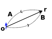
(a)                               

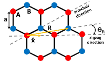
(b)                               

Figure 1: (Color online) Schematic diagrams of (a) the propagating paths of an electron in clean system and (b) the graphene lattice. The two sublattices are denoted as A and B and the two representative directions (zigzag and armchair) are indicated as dashed gray lines. $\theta_{\bm{R}}$ is the angle between the displacement vector of the magnetic impurity $\bm{R}$ and the unit vector $\hat{\bm{x}}$.

Bergmann interpreted the RKKY oscillation as an interference of the conduction electron’s wave function scattered by the magnetic impurity and calculated the interference using the Huygens’ principle in a three-dimensional metal.Bergmann (1987) According to the Huygens’ principle in two dimensions,Cirone et al. (2002) the amplitude of a wave which propagates from a source at position $\bm{R}^{\prime}$ decays with distance and gains a phase factor at a position $\bm{R}$ given by

$$\Psi(\bm{R}^{\prime})\,\frac{e^{i\bm{k}\cdot(\bm{R}-\bm{R}^{\prime})}}{\sqrt{|\bm{R}-\bm{R}^{\prime}|}},$$ (2)

where $\Psi(\bm{R}^{\prime})$ is the amplitude of the wave at the source and the extra factor comes from the asymptotic form of the Bessel function in two dimensions ($e^{ikr}/\sqrt{r}$). If an electron propagates from $\bm{R}$ to the origin in graphene (Fig. 1a), the amplitude gets a phase factor

$$A=\frac{1}{\sqrt{R}}\,\left[e^{i(\bm{K}+\bm{q})\cdot{\bm{R}}}+e^{i(\bm{K}^{\prime}+\bm{q})\cdot{\bm{R}}}\right]e^{i\varepsilon_{q}t/2},$$ (3)

where the wave vector is expanded around the two neighboring Dirac points $\bm{K}$ and $\bm{K}^{\prime}$ with a relative wave vector $\bm{q}$. During its propagation, the electron gets another phase factor, $e^{i\varepsilon_{q}t/2}$, where $\varepsilon_{q}=v_{F}q$ is the kinetic energy of the electron near the Dirac point, $v_{F}$ is the Fermi velocity and $t/2$ is the propagation time from $\bm{R}$ to the origin. After the electron is scattered by a magnetic impurity at the origin, it travels back to the position $\bm{R}$. The amplitude then gains an additional modulation of the amplitude which is given by

$$B=\frac{\delta_{0}}{\sqrt{R}}\,\left[e^{-i(\bm{K}+\bm{q})\cdot{\bm{R}}}+e^{-i(\bm{K}^{\prime}+\bm{q})\cdot{\bm{R}}}\right]e^{i(\varepsilon_{q}t/2+\delta_{0})},$$ (4)

where $\delta_{0}$ depends on the properties of the magnetic impurity at the origin. When the electron goes back to $\bm{R}$, its direction is opposite compared to the first propagation and this is the reason why the signs are opposite in the phase factors in $A$ and $B$. In the time domain, however, it propagates in the same direction so that the phase factor related with the time ($\varepsilon_{q}t/2$) has the same sign. This is consistent with the diagrammatic expression for the RKKY interaction which has two retarded Green’s functions. For a closed path, a loop of the opposite direction makes a contribution with the same weight, so that the modulation of the charge density of an electron which has the energy $\varepsilon_{q}$ is given by

$$\Delta\rho_{\varepsilon}(\bm{R}) = 2|\psi(\bm{R})|^{2}AB$$ (5)

$$= \frac{4\delta_{0}}{V}\frac{1+\cos[(\bm{K}-\bm{K}^{\prime})\cdot\bm{R}]}{R}e^{i\varepsilon_{q}t},$$

such that the total charge modulation is given by

$$\rho(\bm{R}) = \int d\varepsilon\,f(\varepsilon)\,N(\varepsilon)\Delta\rho_{\varepsilon}(\bm{R})$$ (6)

$$= -\frac{\delta_{0}v_{F}^{2}}{V}\frac{1+\cos[(\bm{K}-\bm{K}^{\prime})\cdot\bm{R}]}{R^{d+\alpha}},$$

Here, $|\psi(\bm{R})|^{2}=1/V$ for free electron, $V$ is the volume of the system, $f(\varepsilon)$ is the Fermi-Dirac distribution function, $N(\varepsilon)=|\varepsilon|^{\alpha}$ is the density of state at the Fermi level, $\alpha$ is the pseudogap exponent, $d$ is the spatial dimension, and $t=2r/v_{F}$ is the total time it takes to return to $\bm{R}$.

The total charge density in (Eq. (6)) can be easily related to the RKKY interaction.Bergmann (1987) Since in graphene $d=2$ and $\alpha=1$, the resulting distance dependence is $1/R^{3}$, which is consistent with previous works.Saremi (2007); Black-Schaffer (2010); Sherafati and Satpathy (2011a) We conclude therefore that the existence of the pseudogap at the Dirac point causes the faster spatial decay of the RKKY interactions in graphene compared to conventional two-dimensional system ($d=2$, $\alpha=0$). Even though Eq. (6) does not give detailed information of about the RKKY interactions, such as the sign dependence on the sublattice and an extra phase factor depending on the direction between point $\bm{R}$ and the origin, it agrees with previous results obtained by the Green’s function method,Sherafati and Satpathy (2011a); Kogan (2011) namely,

$$J_{\textrm{AA}}^{0} = -J^{2}\frac{1+\cos[(\bm{K}-\bm{K}^{\prime})\cdot\bm{R}]}{R^{3}},$$ (7)

$$J_{\textrm{AB}}^{0} = J^{2}\frac{3+3\cos[(\bm{K}-\bm{K}^{\prime})\cdot\bm{R}+\pi-2\theta_{R}]}{R^{3}},$$ (8)

where $\theta_{R}$ is an angle between the position vector $\bm{R}$ and the zigzag-AA direction ($\theta_{R}=0)$ as described in Fig. 1b.

III Numerical method

We start with a general expression for the RKKY exchange coupling constant in terms of the off-diagonal matrix elements of the local density of states $\rho_{ij}(E)=\braket{i}{\delta(E-\hat{H})}{j}$,Roche and Mayou (1999); Lee et al. (2012)

$$J_{\textrm{RKKY}}=-J^{2}\frac{S(S+1)}{2S^{2}}\int_{E<\mu}dE\int_{E^{\prime}>\mu}dE^{\prime}\frac{F(E,E^{\prime})}{E-E^{\prime}},$$ (9)

where $F(E,E^{\prime})=\textrm{Re}[\rho_{ij}(E)\rho_{ji}(E^{\prime})]$, $J$ is the local coupling constant between the localized magnetic impurity and the itinerant electrons in the host metal, $S$ is the magnitude of the impurity spin, $i,j$ are the site indices of magnetic impurities located at position $\bm{R}_{i}$ ($\bm{R}_{j}$), and $\mu$ is the Fermi energy. Zero temperature ($T=0$) is assumed. Using the KPM, one may calculate the matrix elements of the local density of state efficiently,Weiße et al. (2006)

$$\rho_{ij}\approx\frac{1}{\pi\sqrt{1-E^{2}}}\left[g_{0}\,m^{ij}_{0}+2\sum^{M}_{l=1}g_{l}\,m^{ij}_{l}\,T_{l}(E)\right],$$ (10)

where $T_{l}(E)$ is the $l$th Chebyshev polynomial of the first kind, $m^{ij}_{l}=\braket{i}{T_{l}(\hat{H})}{j}$, $\hat{H}$ is an electronic Hamiltonian, and $g_{l}$ are the Jackson kernels coefficients. The sum is taken up to a cutoff number $M$. One may obtain the expansion coefficients $m_{l}^{ij}$ using the recurrence relation of Chebyshev polynomials, namely, $T_{l+1}=2\hat{H}T_{l}(\hat{H})-T_{l-1}(\hat{H})$ with $T_{0}(\hat{H})=1$ and $T_{1}(\hat{H})=\hat{H}$. Implicit in Eq. (10) is the normalization of the energy spectrum to a band of unity width.

IV Disordered graphene at half filling ($\mu=0$, $W\neq 0$)

We have investigated the effect of on-site nonmagnetic disorder at the charge neutrality point ($\mu=0,\,W\neq 0$). For each value of $W$, 1600 different disorder configurations were generated and the corresponding matrix elements of the density of state $\rho_{ij}$ (Eq. 10) evaluated through the KPM with a Chebyshev polynomial cutoff number $M=5\times 10^{3}$ on a lattice with $5\times 10^{5}$ sites. We have previously reported that in the diffusive regime ($l_{e}<R<\xi$), which was characterized by determining the mean free path $l_{e}$ and the localization length $\xi$, the armchair direction is the only direction in which the averaged value of the RKKY interaction over disorder configurations does not alter its sign.Lee et al. (2012) To illustrate this effect, we calculated the RKKY interactions along the directions ($\theta_{R}=\pi/12.5,\,\pi/10$) which pass through only the same sublattice and the results are shown in Fig. 2 together with the ones for the zigzag-AA and armchair-AA directions. Notice that the amplitudes of the RKKY interaction are multiplied by the cube of the distance in order to make the effect of nonmagnetic disorder more transparent. As expected from previous studies,de Chatel (1981); Jagannathan et al. (1988); Zyuzin and Spivak (1986); Lerner (1993); Bulaevskii and Panyukov (1986) the amplitude of the averaged interactions decays exponentially over length scales exceeding the mean free path $l_{e}$,

$$\langle J_{\textrm{RKKY}}\rangle_{\textrm{avg}}=J_{\textrm{RKKY}}^{\textrm{clean}}\,e^{-R/l_{e}},$$ (11)

where $\langle O\rangle_{\textrm{avg}}$ indicates averaging over disorder configurations and $J_{\textrm{RKKY}}^{\textrm{clean}}$ is the amplitude of the RKKY interaction in a clean system. On-site disorder breaks the sublattice symmetry. Consequently, the sign of the RKKY interaction between the moments which are localized at the same sublattice fluctuates, allowing both ferromagnetic and antiferromagnetic correlation (Fig. 2a, b, c). The importance of the sublattice symmetry was highlighted in our previous work by considering the hopping disorder.Lee et al. (2012) When randomness is added to the hopping integral $t=t_{0}+\Delta t$ without on-site disorder, it does not break the sublattice symmetry and the RKKY interaction never changes its sign for magnetic moments sitting in either the same or different sublattices, even for a fixed disorder configuration. Interestingly, the averaged RKKY interaction amplitude along the armchair direction with on-site disorder does not change sign (Fig. 2d), while for a particular disorder configuration it randomly changes both sign and amplitude.

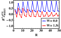
(a)     $\theta_{R}=0$, zigzag-AA    

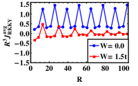
(b)          $\theta_{R}=\pi/12.5$         

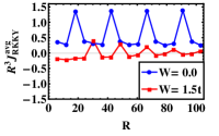
(c)          $\theta_{R}=\pi/10$          

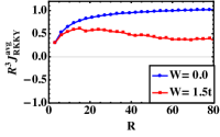
(d) $\theta_{R}=\pi/3$, armchair-AA

Figure 2: (Color online) Plots of the RKKY interaction strength multiplied by the cube of the distance, $R^{3}$, along the (a) $\theta_{R}=0$ (zigzag-AA) (b) $\theta_{R}=\pi/12.5$ (c) $\theta_{R}=\pi/10$ and (d) $\theta_{R}=\pi/3$ (armchair-AA) direction in the diffusive regime, as averaged over 1600 different disorder configurations. A lattice with $5\times 10^{5}$ sites and a polynomial degree cutoff of $M=5\times 10^{3}$ are used in these numerical calculations.

In a dirty metal the charge density is modified by disorder due to the random phase factors. When these random phase factors are simply averaged over disorder configurations, they gain an exponentially decaying factor. Due to the geometrical anisotropy in graphene, the influence of these random phase factors depends on the path direction. According to Feynman’s path integral representation, the coupling is dominated by the shortest path between two magnetic impurities. There always exists an even number of shortest paths along the armchair direction (Fig. 3b), but only one along the zigzag direction (Fig. 3a). Therefore, for the zigzag direction, the electron wave is scattered by the same disorder twice with the same phase (e.g. $\delta_{1}$ in Fig. 3a) when it returns to the origin. However, along the armchair direction, there are closed paths which include different impurities and thereby different scattering phases (e.g. $\delta_{1}$ and $\delta_{2}$ in Fig. 3b). If we average the modulation of the charge density over the phases $\delta_{1}$ and $\delta_{2}$ we find

$$\langle\Delta\rho_{\textrm{zg}}(\bm{R})\rangle=\Delta\rho_{0}\,\langle e^{i2\delta_{1}}\rangle=\Delta\rho_{0}\,e^{-2\langle\delta_{1}^{2}\rangle}\\$$ (12)

and

$$\langle\Delta\rho_{\textrm{arm}}(\bm{R})\rangle = \Delta\rho_{0}\,\langle e^{i2\delta_{1}}+e^{i(\delta_{1}+\delta_{2})}+e^{i2\delta_{2}}\rangle$$ (13)

$$= \Delta\rho_{0}\,[\,2\,e^{-2\langle\delta_{1}^{2}\rangle}+e^{-\langle\delta_{1}^{2}\rangle}\,],$$

where $\langle\cdots\rangle$ is the average over disorder configurations and $\Delta\rho_{0}$ is the modulation of the charge density in the clean system [Eq. (6)]. The modulation along the armchair direction [Eq. (13)] is dominated by the term $\Delta\rho_{0}\,e^{-\langle\delta_{1}^{2}\rangle}$ coming from the closed loop connected by two unrelated paths, so that the average value is exponentially closer to the clean value, while the zigzag direction is dominated by $\Delta\rho_{0}\,e^{-2\langle\delta_{1}^{2}\rangle}$ [Eq. (12)]. In this sense, one may expect the RKKY interaction in the armchair direction to be less sensitive to the nonmagnetic weak disorder than in other directions. This may explain our previous results Lee et al. (2012) and the results shown in Fig. 2, where the averaged value in the armchair direction remains susbstantially larger than in the other directions and does not change its sign.

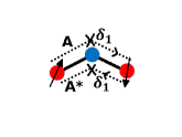
(a) zigzag     

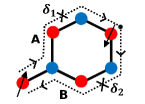
(b) armchair      

Figure 3: (Color online) Schematic diagrams of the shortest path from the origin to the first lattice point along (a) the zigzag-AA direction and (b) the armchair-AA direction. $\delta_{1\,(2)}$ denotes the phase shift due to nonmagnetic disorder and ${\bf A\,(B)}$ denote the modulation of the charge density amplitude.

In order to investigate in more detail how much nonmagnetic disorder affects the RKKY interaction and how the latter depends on direction in the graphene lattice and on particular lattice points, we have calculated the distribution of the interaction amplitude for a disorder strength $W=t$ and at lattice points which are on the zigzag or armchair direction. The results are shown in Fig. 4 a-e. In these calculations, $3\times 10^{4}$ different disorder configurations are used with for a lattice of $2\times 10^{4}$ sites, while the number of Chebyshev polynomials $M=10^{3}$ is fixed. When the distance $R$ between the magnetic impurities is smaller than the mean free path, the RKKY interaction multiplied by the cube of the distance has a shape which does not depend on the distance. Interestingly, the distribution has three different shapes along the zigzag-AA direction (Fig. 4a-c), which are repeated periodically every third site in that direction. However, there is only one type of distribution along the armchair direction, as can be seen in  (Fig. 4d). The oscillating factor in the semiclassical expressions for the charge density, $\cos[(\bm{K}-\bm{K}^{\prime})\cdot\bm{R}]$ in Eq. (6), takes only the values ,$(1,-1/2,-1/2)$ along sites in the zigzag-AA direction. The RKKY interaction on sites which give the same numerical factor, either $1$ or $-1/2$, are found to have the same distribution. In order to directly compare them with each other, we plot together the distributions of the RKKY interactions obtained for these sites in Fig. 4e. The RKKY interaction at sites where the oscillating factor takes the value (-1/2) along the zigzag-AA direction has the broadest (green) distribution, while the RKKY interaction at site where the oscillating factor takes the value (1) has the narrowest (red) distribution.

The unaveraged RKKY interaction, i.e., that obtained for a particular disorder representation, is found to remain long ranged as in the clean system. However, we find that the oscillations acquire a random phase that also changes with the distance $R$ between magnetic impurities. Therefore, the average value does not characterize the RKKY interaction at distances exceeding the mean free path. To find the typical value, we evaluated the geometrical average of the interaction amplitude, which is defined by

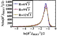
(a)           zigzag1            

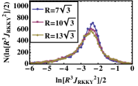
(b)           zigzag2            

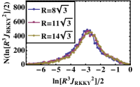
(c)           zigzag3            

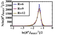
(d)          armchair            

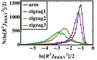
(e)                                 

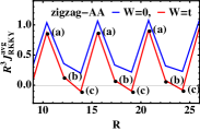
(f)                               

Figure 4: (Color online) Plots of the distribution of the RKKY interaction amplitude ($\sqrt{J_{\textrm{RKKY}}^{2}}$) multiplied by the cube of distance, $R^{3}$, for the (a) first (b) second (c) third of the triplet of points along zigzag-AA direction (see Fig. 4 f for the definition of these points), and (d) for the armchair direction. The disorder strength is fixed to $W=t$. For comparison, these distributions are plotted together in (e). A lattice with $2\times 10^{4}$ sites and a polynomial degree cutoff of $M=10^{3}$ are used. The lattice constant $a$ is set to unity.

$$J_{\textrm{RKKY}}^{\textrm{geo}}\equiv\exp\Big{[}\frac{1}{2}\langle\,\ln(J_{\textrm{RKKY}})^{2}\,\rangle_{\textrm{avg}}\Big{]}.$$ (14)

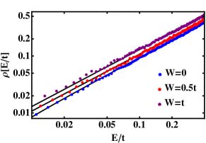
(a)                                                     

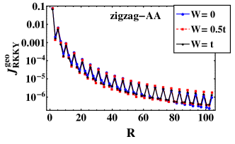
(b)                                                     

Figure 5: (Color online) (a) The averaged density of states in a double logarithmic plot (b) and the geometrical averaged RKKY interactions along the zigzag-AA direction. For the density of state calculation, a lattice with $3\times 10^{7}$ sites and a polynomial degree cutoff of $M=7\times 10^{3}$ are used. For the RKKY interaction calculation, the same lattice size and polynomial cutoff of Fig. 2 are used. The black lines in (a) represent fittings to the relation $\rho(E)=\gamma|E|$ with $\gamma=0.95,\,1.07,\,1.3$ for $W=0,\,0.5t,t$, respectively.

The typical value is found to have the same power-law decaying behavior with distance as the amplitude of the RKKY interaction in the clean limit.Zyuzin and Spivak (1986); Bergmann (1987); Lerner (1993); Sobota et al. (2007); Bulaevskii and Panyukov (1986) Before a direct evaluation of the geometrical average, we have calculated the density of state for two disorder strengths  $W=0.5t,t$ to observe how weak disorder affects the pseudogap at the neutrality point ($E=0$), since, as we have seen above, the power of the pseudogap is directly related to the unconventional power-law decay of the RKKY interaction. For the density-of-states calculation, we used the KPM Weiße et al. (2006); Amini et al. (2009) method with $3\times 10^{7}$ sites and a polynomial degree cutoff of $M=7\times 10^{3}$. As one may see from the plot of the density of states in  (Fig. 5a), the pseudogap is still not filled for weak disorder, has the same power law as in the clean limit, and only the slope around the neutrality point is changed,Amini et al. (2009)

$$\rho(E)=\gamma|E|,$$ (15)

where $\rho(E)$ is the density of states and $E$ is the energy measured in units of the hopping amplitude $t$. The slope $\gamma$ depends on the disorder strength and is obtained by fitting the data in Fig. 6.

Using the Born and T-matrix approximations, an analytical study has reported that there is a logarithmic correction to the density of states around the neutrality point, yielding $\rho(E)=|E|\ln|E|$ in the presence of disorder.Hu et al. (2008) This logarithm correction does not change the power of the distance dependence of the RKKY interaction [Eq.(6)]. Consequently, the geometrical average of the RKKY interaction is expected to have the same power-law exponent as the clean system ($1/R^{3}$). The direct numerical calculation shown in Fig. 5b strongly supports this conclusion.

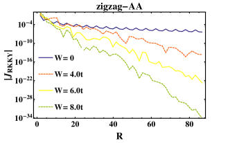
(a)                                                     

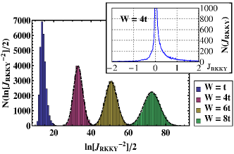
(b)                                                     

Figure 6: (Color online) Plots of (a) the absolute value of the RKKY interaction in a disordered sample as a function of distance and (b) of the distribution of the logarithm of the RKKY interaction amplitude for $R=50\sqrt{3}a$ and different disorder strengths. The inset of (b) shows the distribution of the amplitude itself for $W=4t$. A lattice with $1.8\times 10^{5}$ sites and a polynomial degree cutoff of $M=3\times 10^{3}$ are used. The black dashed lines represent the resulting distribution functions with $\sigma=2.4,\,3.2,\,4.35$ and $\alpha=32.5,\,50,\,72.5$ for $W=4t,\,6t,\,8t$, respectively (see text).

Figure 6a shows how the RKKY interaction in a strongly disordered sample gets suppressed by several orders of magnitude when the strength of the nonmagnetic random potential is increased. In order to investigate the broadening of the distribution, we employed $3\times 10^{4}$ realizations of the disorder potential and calculated the RKKY interaction amplitude for a fixed distance $R=50\sqrt{3}$. The results are shown in Fig. 6b. The inset indicates that the interaction strength follows a distribution with very long assymetric tails. The squared amplitude ($J_{\textrm{RKKY}}^{2}$) has a distribution similar to log-normal with a width that increases with disorder strength. Using a field-theoretical approach valid in the metallic regime, Lerner found Lerner (1993) that the increase in the strength of the nonmagnetic disorder leads to a crossover in the shape of the distribution function from a broad non-Gaussian with the very long tails in the weak disorder regime to a completely log-normal distribution in the region of strong disorder regime. This may explain the crossover of the distribution which we observe from weak disorder $W=t$ to strong disorder  ($W=4t,\,6t,\,8t$). In order to directly compare we have fitted the results with a log-normal functional form, which is given by

$$P(x)=\frac{N}{\sqrt{2\pi\sigma^{2}}}\,\exp\Big{[}-\frac{(x-\alpha)^{2}}{2\sigma^{2}}\Big{]},$$ (16)

where $N=3\times 10^{4}$ is the number of realizations and $x=\ln[J_{\textrm{RKKY}}^{-2}]/2$. The data are shown together with the fitting curves in Fig. 6b (black dashed lines).

The width $\sigma$ of the distribution in Eq. (16) has been analyzed as functions of the disorder strength $W$ and is shown in Fig. 7. The red line in Fig. 7 is a linear fitting curve ($\sigma=W/2+0.34$) and agrees with the analytical prediction by Lerner, who has used the renormalization group method to obtain Lerner (1993)

$$\sigma\sim 1/\sqrt{l_{e}}\sim W,$$ (17)

where $l_{e}\sim 1/W^{2}$ is the mean free path of electrons, which we studied in our previous work.Lee et al. (2012)

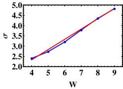
Figure 7: (Color online) Plot of the width of the distribution of RKKY interaction amplitudes as a function of the disorder strength $W$ (in unit of $t$). The red line represents a linear fitting curve  which yields $\sigma=W/2+0.34$.

V Doped graphene ($\mu\neq 0$)

V.1 Clean system ($W=0$)

By controlling $\mu$ in the Hamiltonian of Eq. (1), we investigate how the RKKY interaction evolves with the Fermi level. Results are shown in Fig. 8, where the interaction amplitude is multiplied by $R^{2}$ in order to emphasize its oscillatory behavior. In these calculations, we used a lattice with $7.2\times 10^{5}$ sites and a polynomial degree cutoff $M=3\times 10^{3}$. Near the neutrality point a beating pattern appears as shown in Fig. 8a, b. It consists of a superposition of waves with the wave vectors $\bm{K}-\bm{K}^{\prime}$ and $\bm{q}_{F}$, where $\bm{q}_{F}$ is the Fermi wave vector originating from the Friedel oscillations at finite Fermi energy. Recently, the following analytical expressions for the beating pattern were derived using lattice Green’s functions:Sherafati and Satpathy (2011a)

$$J_{\textrm{AA}}=J_{\textrm{AA}}^{0}\bigg{[}1+\frac{8q_{F}R}{\sqrt{\pi}}G_{1,3}^{2,0}\left(\begin{matrix}\frac{1}{2},\frac{3}{2}\\ 1,1,1\end{matrix};q_{F}^{2}R^{2}\right)\bigg{]}$$ (18)

and

$$J_{\textrm{AB}}=J_{\textrm{AB}}^{0}\bigg{[}1-\frac{8q_{F}R}{\sqrt{3\pi}}G_{2,4}^{2,1}\left(\begin{matrix}\frac{1}{2},\frac{3}{2}\\ 1,2,0,-\frac{1}{2}\end{matrix};q_{F}^{2}R^{2}\right)\bigg{]},$$ (19)

where $J^{0}_{\textrm{AA(B)}}$ is the RKKY coupling function at the neutrality point [see Eq. (8)] and $G$ is the Meijer-G function. Note that term within brackets describes the isotropic dependence of the oscillations on the Fermi momentum $\bm{q}_{F}$. The external prefactor, $J^{0}_{\textrm{AA(B)}}$, on the contrary, is strongly anisotropic, depending on the vector given by the momentum difference between the two neighbored Dirac points $\bm{K}-\bm{K}^{\prime}$. To make a comparison with our calculations, the function represented by Eq. (19) is also presented in Fig. 8 by a red dashed line. Excellent agreement is found. One can estimate the wavelength of the long oscillation, which appears at finite Fermi level, using the dispersion relation near the neutrality point, which is given by

$$E(\bm{q})=v_{F}|\bm{q}|,$$ (20)

where $\bm{q}$ is the momentum relative to the Dirac point and $v_{F}=3ta/2$ is the Fermi velocity.Castro Neto et al. (2009) The Fermi wavelength is found to be about $\lambda_{F}\approx 50a$ for $\mu=0.1t$. This coincides with the period seen in  (Fig. 8a). As expected from Eq. (19), the oscillations with large period seen in (Fig. 8b) are isotropic.

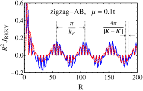
(a)                                              

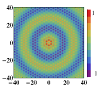
(b)                            

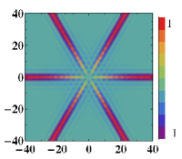
(c)                            

Figure 8: (Color online) (a) The RKKY interaction amplitude multiplied by $R^{2}$ in doped graphene at the chemical potential $\mu=0.1t$ along the zigzag-AB direction. Density plots of the RKKY interaction amplitude for (b) $\mu=0.2t$ and (c) $\mu=t$ for all directions. In (a), the result of culations used the kernel polynomial method and the lattice Green’s function method are represented as solid blue and dashed red line, respectively. A lattice with $7.2\times 10^{5}$ sites and a polynomial degree cutoff of $M=5\times 10^{3}$ were used. The lattice constant $a$ is set to unity.

We have also calculated the RKKY interaction amplitude for highly doped graphene ($\mu=t$). The results are multiplied by the square of the distance, $R^{2}$, and are shown in the density plots of  (Fig. 8c). The behavior cannot be described by Eqs. (18) and (19) which are valid only close to the neutrality point. When the Fermi level is exactly at the van Hove singularity at  ($\mu=t$), the ordering pattern of the RKKY interactions along the zigzag direction is reversed. In other words, the correlation between impurities on zigzag-AA or BB is always antiferromagnetic and ferromagnetic for zigzag-AB or BA pairs. At the same time, the interactions are strongly suppressed for the other directions. This is in accordance with a result of a previous study.Uchoa et al. (2011)

V.2 Disordered system ($W\neq 0$)

We have also calculated the RKKY interaction amplitude in disordered doped graphene and the results are shown in Fig. 9. A lattice with $5\times 10^{5}$ sites and a polynomial degree cutoff of $M=5\times 10^{3}$ were used in these numerical calculations. In our previous work,Lee et al. (2012) we reported that the amplitude of the averaged RKKY interaction along the zigzag-AA direction in the ballistic regime ($R<l_{e}$) increases with weak disorder (Fig. 4f). Even though the unusual oscillation coming from the interference of two Dirac points still exists (Fig. 9a), the amplitude of the envelope of the averaged RKKY interaction decreases with disorder strength $W$ and the period ($2\pi/k_{\textrm{F}}$) of the oscillation coming from the finite Fermi energy is modified by the disorder as in a conventional metal.

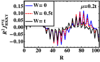
(a)                                 

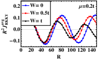
(b)                                 

Figure 9: (Color online) The average RKKY interaction strength multiplied by the square of the distance, $R^{2}$, along the (a) zigzag-AA and (b) armchair-AA directions at the Fermi energy $\mu=0.2t$ is plotted in the diffusive regime. 1600 different disorder configurations are used in the averaging. The same lattice size and polynomial cutoff as in Fig. 2 were used.

VI Discussion and Conclusions

In conclusion, we have employed a semiclassical description of the RKKY interaction in terms of the modulation of the charge density by the presence of magnetic impurities in order to rederive an analytical expression applicable to pure graphene. This semiclassical approach provides not only a simpler derivation, but also an intuitive interpretation of the origin of the oscillating behavior of the RKKY interaction at zero doping as an interference of the two degenerate Dirac points. Moreover, the origin of the unusual power-law decay of the RKKY interaction in pure graphene at the neutrality point is clearly related to the pseudogap in the density of states. Using a Feynman’s path integral scheme, we could also trace the origin of the anisotropic sensitivity of the RKKY interaction to disorder to the presence of multiple shortest paths between two magnetic impurities in the armchair direction, showing that this direction is more robust to disorder than the zigzag one.

As an extension of our previous study,Lee et al. (2012) we have calculated and studied the RKKY interaction in doped and disordered graphene in detail using the kernel polynomial method. Fnite gate voltage breaks particle-hole symmetry and the resulting finite Fermi surface yields Friedel oscillations, so that the sign of the RKKY interaction between the impurities localized on the same sublattice now oscillates with distance. When the Fermi level is exactly at the van Hove singularity ($\mu=t$), the ordering pattern of the RKKY interactions along the zigzag direction is reversed. At the same time, the interactions are strongly suppressed for all other directions.

In order to study the anisotropic influence of nonmagnetic disorder, we evaluated the RKKY interactions along two different directions between the zigzag and armchair directions. As reported in our previous study and expected from the semiclassical approach, in the diffusive regime the armchair direction is not affected by the nonmagnetic disorder as much as the other directions. We have also found that, in the ballistic regime ($R<l_{e}$), the distribution of the RKKY interactions along the zigzag direction is not universal but depends on the lattice sites at which the pair of magnetic impurities sit. We identified three different representative shapes, which repeat themselves periodically. By an accurate evaluation of the density of states around the neutrality point in weakly disordered regime ($W\leq t$), we confirmed that the linear dispersion relation is still valid and the pseudogap is not filled. This is in full agreement with the fact that the geometrical average of the RKKY interaction in the diffusive regime decays as in the clean system, namely, as $1/R^{3}$, and not as $1/R^{2}$, which is the usual behavior for two-dimensional metals. In the localized regime ($R>\xi$), the geometrical average is also exponentially suppressed at distances exceeding the localization length $\xi$ and the distribution of the strength of the RKKY interaction shows a crossover from the non-Gaussian shape with very long tails to the completely log-normal form when increasing the disorder strength. We have analyzed the width of the log-normal distribution and confirmed that it increases linearly with the amplitude of the disorder potential $W$.

In this work we showed that the KPM method is efficient and accurate for studying interactions in disordered systems. In order to minimize the computation time while keeping the highest accuracy, the convergence of the calculations with respect to the Chebyshev polynomial cutoff degree $M$ and the system size $L$ have been investigated in detail (see Appendix A). The proper cutoff $M$ to reach convergence is found to increase linearly with the distance $R$ between two magnetic impurities, as seen in Fig. 10 b. For a given distance $R$, a system size $L$ about five times larger than $R$ is found to give convergent results. In comparison with the exact numerical diagonalization, the KPM is found to be much faster. It can be implemented for very large system sizes, even in disordered ones, where thousands of realizations are needed in order to yield meaningfull statistics.

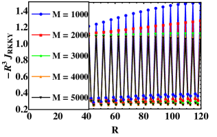
(a)                                                         

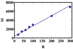
(b)                                             

Figure 10: (Color online) Plots of (a) the RKKY interaction as function of the polynomial degree $M$ in a lattice with $5\times 10^{5}$ sites. (b) The smallest cutoff number $M$ that yields a convergent result as function of the distance between the magnetic impurities $R$.

Appendix A Convergence of the Kernel Polynomial Method Calculations

When using the KPM, the calculation of the Chebyshev polynomials using recurrence relations consumes most of the computation time. Therefore, we investigated first the relation between the cutoff number $M$ and the convergence of the results in order to be able to minimize $M$ and optimize the calculations. For clean graphene, a lattice with $5\times 10^{5}$ sites was used in these calculations. When a cutoff number $M$ is not sufficient, the amplitude of the RKKY interaction deviates from the expected power-law behavior, as indicated by the blue and red lines in Fig. 10a). When we determined the smallest cutoff number $M$ such that the variance of the amplitude of the RKKY interaction is less than 5%, we found that it increases linearly with the distance between two magnetic impurities $R$ as seen in Fig. 10b). This linear relation between the distance and the cutoff number allows the rapid calculation of the RKKY interaction amplitude between the magnetic moments even at large distances $R$.

In order to minimize the KPM calculation time further, we have also studied the smallest system size $L$ which yields convergent results, as shown in Fig. 11. $R_{F}$ denotes the longest distance used in the calculation, $R_{F}=50\sqrt{3}a$ and the cutoff number is $M=5\times 10^{3}$. One can observe a good convergent behavior (see green and black line in Fig. 11) when the system size $L$ is larger than $5R_{F}$. The exact diagonalization method also yields a proper result when $L=5R_{F}$.Black-Schaffer (2010) However, the KPM does not require matrix diagonalization and therefore is a much faster computational tool.

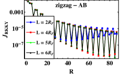
(a)

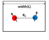
(b)

Figure 11: (Color online) Plots of the RKKY interaction in terms of a system size $L$. $50\sqrt{3}a$ is used as the longest distance $R_{F}$. A cutoff number $M=5\times 10^{3}$ is used in these calculations.