Optimal Orthogonal Graph Drawing with Convex Bend Costs

Abstract

Traditionally, the quality of orthogonal planar drawings is quantified by either the total number of bends, or the maximum number of bends per edge. However, this neglects that in typical applications, edges have varying importance. Moreover, as bend minimization over all planar embeddings is $\mathcal{NP}$-hard, most approaches focus on a fixed planar embedding.

We consider the problem OptimalFlexDraw that is defined as follows. Given a planar graph $G$ on $n$ vertices with maximum degree 4 and for each edge $e$ a cost function $\operatorname{cost}_{e}\colon\mathbb{N}_{0}\longrightarrow\mathbb{R}$ defining costs depending on the number of bends on $e$, compute an orthogonal drawing of $G$ of minimum cost. Note that this optimizes over all planar embeddings of the input graphs, and the cost functions allow fine-grained control on the bends of edges.

In this generality OptimalFlexDraw is $\mathcal{NP}$-hard. We show that it can be solved efficiently if 1) the cost function of each edge is convex and 2) the first bend on each edge does not cause any cost (which is a condition similar to the positive flexibility for the decision problem FlexDraw). Moreover, we show the existence of an optimal solution with at most three bends per edge except for a single edge per block (maximal biconnected component) with up to four bends. For biconnected graphs we obtain a running time of $\mathcal{O}(n\cdot T_{\operatorname{flow}}(n))$, where $T_{\operatorname{flow}}(n)$ denotes the time necessary to compute a minimum-cost flow in a planar flow network with multiple sources and sinks. For connected graphs that are not biconnected we need an additional factor of $\mathcal{O}(n)$.

1 Introduction

Orthogonal graph drawing is one of the most important techniques for the human-readable visualization of complex data. Its æsthetic appeal derives from its simplicity and straightforwardness. Since edges are required to be straight orthogonal lines—which automatically yields good angular resolution and short links—the human eye may easily adapt to the flow of an edge. The readability of orthogonal drawings can be further enhanced in the absence of crossings, that is if the underlying data exhibits planar structure. Unfortunately, not all planar graphs have an orthogonal drawing in which each edge may be represented by a straight horizontal or vertical line. In order to be able to visualize all planar graphs nonetheless, we allow edges to have bends. Since bends obfuscate the readability of orthogonal drawings, however, we are interested in minimizing the number of bends on the edges.

In this paper we consider the problem OptimalFlexDraw whose input consists of a planar graph $G$ with maximum degree 4 and for each edge $e$ a cost function $\operatorname{cost}_{e}\colon\mathbb{N}_{0}\longrightarrow\mathbb{R}$ defining costs depending on the number of bends on $e$. We seek an orthogonal drawing of $G$ with minimum cost. Garg and Tamassia [9] show that it is $\mathcal{NP}$-hard to decide whether a 4-planar graph admits an orthogonal drawing without any bends. Note that this directly implies that OptimalFlexDraw is $\mathcal{NP}$-hard in general. For a special case, namely planar graphs with maximum degree 3 and series-parallel graphs, Di Battista et al. [4] give an algorithm minimizing the total number of bends optimizing over all planar embeddings. They introduce the concept of spirality that is similar to the rotation we use (see Section 2.3 for a definition). Bläsius et al. [2] show that the existence of a planar 1-bend drawing can be tested efficiently. More generally, they consider the problem FlexDraw, where each edge has a flexibility specifying its allowed number of bends. For the case that all flexibilities are positive, they give a polynomial-time algorithm for testing the existence of a valid drawing.

As minimizing the number of bends for 4-planar orthogonal drawings is $\mathcal{NP}$-hard, many results use the topology-shape-metrics approach initially fixing the planar embedding. Tamassia [15] describes a flow network for minimizing the number of bends. This flow network can be easily adapted to also solve OptimalFlexDraw even for the case where the first bend may cause cost, however, the planar embedding has to be fixed in advanced. Biedl and Kant [1] show that every plane graph can be embedded with at most two bends per edge except for the octahedron. Morgana et al. [12] give a characterization of plane graphs that have an orthogonal drawing with at most one bend per edge. Tayu et al. [17] show that every series-parallel graph can be drawn with at most one bend per edge. All these results and the algorithm we present here have the requirement of maximum degree 4 in common. Although this is a strong restriction it is important to consider this case since algorithms dealing with higher-degree vertices (drawing them as boxes instead of single points) rely on algorithms for graphs with maximum degree 4 [16, 8, 11].

Even though fixing an embedding allows to efficiently minimize the total number of bends (with this embedding), this neglects that the choice of a planar embedding may have a huge impact on the number of bends in the resulting drawing. The result by Bläsius et al. [2] concerning the problem FlexDraw takes this into account and additionally allows the user to control the final drawing, for example by allowing few bends on important edges. However, if such a drawing does not exist, the algorithm solving FlexDraw does not create a drawing at all and thus it cannot be used in a practical application. Thus, the problem OptimalFlexDraw, which generalizes the corresponding optimization problem, is of higher practical interest, as it allows the user to take control of the properties of the final drawing within the set of feasible drawings. Moreover, it allows a more fine-grained control of the resulting drawing by assigning high costs to bends on important edges.

Contribution and Outline.

Our main result is the first polynomial-time bend-optimization algorithm for general 4-planar graphs optimizing over all embeddings. Previous work considers only restricted graph classes and unit costs. We solve OptimalFlexDraw if 1) all cost functions are convex and 2) the first bend is for free. We note that convexity is indeed quite natural, and that without condition 2) OptimalFlexDraw is $\mathcal{NP}$-hard, as it could be used to minimize the total number of bends over all embeddings, which is known to be $\mathcal{NP}$-hard [9].

In particular, our algorithm allows to efficiently minimize the total number of bends over all planar embeddings, where one bend per edge is free. Note that this is an optimization version of FlexDraw where each edges has flexibility 1, as a drawing with cost 0 exists if and only if FlexDraw has a valid solution. Moreover, as it is known that every 4-planar graph has an orthogonal representation with at most two bends per edge [1], our result can also be used to create such a drawing minimizing the number of edges having two bends by setting the costs for three or more bends to $\infty$.

To derive the algorithm for OptimalFlexDraw, we show the existence of an optimal solution with at most three bends per edge except for a single edge per block with up to four bends, confirming a conjecture of Rutter [14].

Our strategy for solving OptimalFlexDraw for biconnected graphs optimizing over all planar embedding is the following. We use dynamic programming on the SPQR-tree of the graph, which is a data structure representing all planar embeddings of a biconnected graph. Every node in the SPQR-tree corresponds to a split component and we compute cost functions for these split components determining the cost depending on how strongly the split component is bent. We compute such a cost function from the cost functions of the children using a flow network similar to the one described by Tamassia [15]. As computing flows with minimum cost is $\mathcal{NP}$-hard for non-convex costs we need to ensure that not only the cost functions of the edges but also the cost functions of the split components we compute are convex. However, this is not true at all, see Figure 1 for an example. This is not even true if every edge can have a single bend for free and then has to pay cost 1 for every additional bend, see Figure 1(c). To solve this problem, we essentially show that it is sufficient to compute the cost functions on the small interval $[0,3]$. We can then show that the cost functions we compute are always convex on this interval.

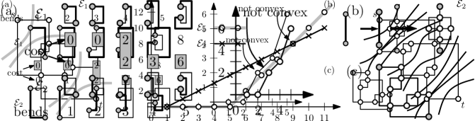
Figure 1: (a) Two parallel edges, the thin has one bend for free, every additional bend costs 1, the thick edge has two bends for free, every additional bend costs 2. Whether embedding $\mathcal{E}_{1}$ or $\mathcal{E}_{2}$ is better depends on the number of bends. The minimum (marked by gray boxes) yields a non-convex cost function. (b) The non-convexity in (a) does not rely on multiple edges, the thick edge could be replaced by the shown gadget where each edge of the gadget has one bend for free and every additional bend costs 2. (c) This example has a non-convex cost function even if every edge has one bend for free and each additional bend costs 1.

We start with some preliminaries in Section 2. Afterwards, we first consider the decision problem FlexDraw for the case that the planar embedding is fixed in Section 3. In this restricted setting we are able to prove the existence of valid drawings with special properties. Bläsius et al. [2] show that “rigid” graphs do not exist in this setting in the sense that a drawing that is bent strongly can be unwound under the assumption that the flexibility of every edge is at least 1. In other words this shows that graphs with positive flexibility behave similar to single edges with positive flexibility. We present a more elegant proof yielding a stronger result that can then be used to reduce the number of bends of every edge down to three (at least for biconnected graphs and except for a single edge on the outer face). In Section 4 we extend the term “bends”, originally defined for edges, to split components and show that in a biconnected graph the split components corresponding to the nodes in its SPQR-tree can be assumed to have only up to three bends. In Section 5 we show that these results for the decision problem FlexDraw can be extended to the optimization problem OptimalFlexDraw. With this result we are able to drop the fixed planar embedding (Section 6). We first consider biconnected graphs in Section 6.1 and compute cost functions on the interval $[0,3]$, which can be shown to be convex on that interval, bottom up in the SPQR-tree. In Section 6.2 we extend this result to connected graphs using the BC-tree (see Section 2.2 for a definition).

2 Preliminaries

In this section we introduce some notations and preliminaries.

2.1 FlexDraw

The original FlexDraw problem asks for a given 4-planar graph $G=(V,E)$ with a function $\operatorname{flex}\colon E\longrightarrow\mathbb{N}_{0}\cup\{\infty\}$ assigning a flexibility to every edge whether an orthogonal drawing of $G$ exists such that every edge $e\in E$ has at most $\operatorname{flex}(e)$ bends. Such a drawing is called a valid drawing of the FlexDraw instance. The problem OptimalFlexDraw is the optimization problem corresponding to the decision problem FlexDraw and is defined as follows. Let $G=(V,E)$ be a 4-planar graph together with a cost function $\operatorname{cost}_{e}:\mathbb{N}_{0}\longrightarrow\mathbb{R}\cup\{\infty\}$ associated with every edge $e\in E$ having the interpretation that $\rho$ bends on the edge $e$ cause $\operatorname{cost}_{e}(\rho)$ cost. Then the cost of an orthogonal drawing of $G$ is the total cost summing over all edges. A drawing is optimal if it has the minimum cost among all orthogonal drawings of $G$. The task of the optimization problem OptimalFlexDraw is to find an optimal drawing of $G$.

Since OptimalFlexDraw contains the $\mathcal{NP}$-hard problem FlexDraw, it is $\mathcal{NP}$-hard itself. However, FlexDraw is efficiently solvable for instances with positive flexibility, that is instances in which the flexibility of every edge is at least 1. To obtain a similar result for OptimalFlexDraw we have to restrict the possible cost functions slightly.

For a cost function $\operatorname{cost}_{e}(\cdot)$ we define the difference function $\Delta\operatorname{cost}_{e}(\cdot)$ to be $\Delta\operatorname{cost}_{e}(\rho)=\operatorname{cost}_{e}(\rho+1)-\operatorname{cost}_{e}(\rho)$. A cost function is monotone if its difference function is greater or equal to 0. We say that the base cost of the edge $e$ with monotone cost function is $b_{e}=\operatorname{cost}_{e}(0)$. The flexibility of an edge $e$ with monotone cost function is defined to be the largest possible number of bends $\rho$ for which $\operatorname{cost}_{e}(\rho)=b_{e}$. As before, we say that an instance $G$ of OptimalFlexDraw has positive flexibility if all cost functions are monotone and the flexibility of every edge is positive. Unfortunately, we have to restrict the cost functions further to be able to solve OptimalFlexDraw efficiently. The cost function $\operatorname{cost}_{e}(\cdot)$ is convex, if its difference function is monotone. We call an instance of OptimalFlexDraw convex, if every edge has positive flexibility and each cost function is convex. Note that this includes that the cost functions are monotone. We provide an efficient algorithm solving OptimalFlexDraw for convex instances.

2.2 Connectivity, BC-Tree and SPQR-Tree

A graph is connected if there exists a path between any pair of vertices. A separating $k$-set is a set of $k$ vertices whose removal disconnects the graph. Separating 1-sets and 2-sets are cutvertices and separation pairs, respectively. A connected graph is biconnected if it does not have a cut vertex and triconnected if it does not have a separation pair. The maximal biconnected components of a graph are called blocks. The cut components with respect to a separation $k$-set $S$ are the maximal subgraphs that are not disconnected by removing $S$.

The block-cutvertex tree (BC-tree) $\mathcal{B}$ of a connected graph is a tree whose nodes are the blocks and cutvertices of the graph, called B-nodes and C-nodes, respectively. In the BC-tree a block $B$ and a cutvertex $v$ are joined by an edge if $v$ belongs to $B$. If an embedding is chosen for each block, these embeddings can be combined to an embedding of the whole graph if and only if $\mathcal{B}$ can be rooted at a B-node such that the parent of every other block $B$ in $\mathcal{B}$, which is a cutvertex, lies on the outer face of $B$.

We use the SPQR-tree introduced by Di Battista and Tamassia [5, 6] to represent all planar embeddings of a biconnected planar graph $G$. The SPQR-tree $\mathcal{T}$ of $G$ is a decomposition of $G$ into its triconnected components along its split pairs where a split pair is either a separation pair or an edge. We first define the SPQR-tree to be unrooted, representing embeddings on the sphere, that is planar embeddings without a designated outer face. Let $\{s,t\}$ be a split pair and let $H_{1}$ and $H_{2}$ be two subgraphs of $G$ such that $H_{1}\cup H_{2}=G$ and $H_{1}\cap H_{2}=\{s,t\}$. Consider the tree containing the two nodes $\mu_{1}$ and $\mu_{2}$ associated with the graphs $H_{1}+\{s,t\}$ and $H_{2}+\{s,t\}$, respectively. These graphs are called skeletons of the nodes $\mu_{i}$, denoted by $\operatorname{skel}(\mu_{i})$ and the special edge $\{s,t\}$ is said to be a virtual edge. The two nodes $\mu_{1}$ and $\mu_{2}$ are connected by an edge, or more precisely, the occurrence of the virtual edges $\{s,t\}$ in both skeletons are linked by this edge. Now a combinatorial embedding of $G$ uniquely induces a combinatorial embedding of $\operatorname{skel}(\mu_{1})$ and $\operatorname{skel}(\mu_{2})$. Furthermore, arbitrary and independently chosen embeddings for the two skeletons determine an embedding of $G$, thus the resulting tree can be used to represent all embeddings of $G$ by the combination of all embeddings of two smaller planar graphs. This replacement can of course be applied iteratively to the skeletons yielding a tree with more nodes but smaller skeletons associated with the nodes. Applying this kind of decomposition in a systematic way yields the SPQR-tree as introduced by Di Battista and Tamassia [5, 6]. The SPQR-tree $\mathcal{T}$ of a biconnected planar graph $G$ contains four types of nodes. First, the P-nodes having a bundle of at least three parallel edges as skeleton and a combinatorial embedding is given by any ordering of these edges. Second, the skeleton of an R-node is triconnected, thus having exactly two embeddings [18], and third, S-nodes have a simple cycle as skeleton without any choice for the embedding. Finally, every edge in a skeleton representing only a single edge in the original graph $G$ is formally also considered to be a virtual edge linked to a Q-node in $\mathcal{T}$ representing this single edge. Note that all leaves of the SPQR-tree $\mathcal{T}$ are Q-nodes. Besides from being a nice way to represent all embeddings of a biconnected planar graph, the SPQR-tree has only size linear in $G$ and Gutwenger and Mutzel [10] showed how to compute it in linear time. Figure 2 shows a biconnected planar graph together with its SPQR-tree.

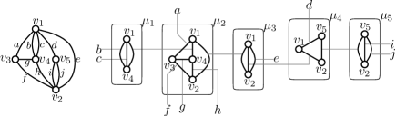
Figure 2: The unrooted SPQR-tree of a biconnected planar graph. The nodes $\mu_{1}$, $\mu_{3}$ and $\mu_{5}$ are P-nodes, $\mu_{2}$ is an R-node and $\mu_{4}$ is an S-node. The Q-nodes are not shown explicitely.

Often the SPQR-tree $\mathcal{T}$ of a biconnected planar graph $G$ is assumed to be rooted in a Q-node representing all planar embeddings with the corresponding edge on the outer face. In contrast to previous results, we assume the SPQR-tree $\mathcal{T}$ to be rooted in some node $\tau$, which may be a Q-node or an inner node. In the following we describe the interpretation of the SPQR-tree with root $\tau$. Every node $\mu$, apart form $\tau$ itself, has a unique parent and thus its skeleton $\operatorname{skel}(\mu)$ contains a virtual edge corresponding to this parent. We refer to this virtual edge as the parent edge. A planar embedding $\mathcal{E}$ of $G$ is represented by $\mathcal{T}$ with root $\tau$ if the embedding induced on the skeleton $\operatorname{skel}(\mu)$ of every node $\mu\not=\tau$ has the parent edge on the outer face. The embedding of $\operatorname{skel}(\tau)$ is not restricted, thus the choice of the outer face makes a difference for the root.

For every node $\mu$ in the SPQR-tree $\mathcal{T}$ apart from the root $\tau$ we define the pertinent graph of $\mu$, denoted by $\operatorname{pert}(\mu)$, as follows. The pertinent graph of a Q-node is the edge associated to it. The pertinent graph of an inner node $\mu$ is recursively defined to be the graph obtained by replacing all virtual edges apart from the parent edge by the pertinent graphs of the corresponding children in $\mathcal{T}$. The expansion graph of a virtual edge $\varepsilon$ in $\operatorname{skel}(\mu)$ is the pertinent graph of $\mu^{\prime}$ where $\mu^{\prime}$ is the child of $\mu$ corresponding to the virtual edge $\varepsilon$ with respect to the root $\mu$.

2.3 Orthogonal Representation

Two orthogonal drawings of a 4-planar graph $G$ are equivalent, if they have the same topology, that is the same planar embedding, and the same shape in the sense that the sequence of right and left turns is the same in both drawings when traversing the faces of $G$. To make this precis, we define orthogonal representations, originally introduced by Tamassia [15], as equivalence classes of this equivalence relation between orthogonal drawings. To ease the notation we first only consider the biconnected case.

Let $\Gamma$ be an orthogonal drawing of a biconnected 4-planar graph $G$. In the planar embedding $\mathcal{E}$ induced by $\Gamma$ every edge $e$ is incident to two different faces, let $f$ be one of them. When traversing $f$ in clockwise order (counter-clockwise if $f$ is the outer face) $e$ may have some bends to the right and some bends to the left. We define the rotation of $e$ in the face $f$ to be the number of bends to the right minus the number of bends to the left and denote the resulting value by $\operatorname{rot}(e_{f})$. Similarly, every vertex $v$ is incident to several faces, let $f$ be one of them. Then we define the rotation of $v$ in $f$, denoted by $\operatorname{rot}(v_{f})$, to be $1$, $-1$ and $0$ if there is a turn to the right, a turn to the left and no turn, respectively, when traversing $f$ in clockwise direction (counter-clockwise if $f$ is the outer face). The orthogonal representation $\mathcal{R}$ belonging to $\Gamma$ consists of the planar embedding $\mathcal{E}$ of $G$ and all rotation values of edges and vertices, respectively. It is easy to see that every orthogonal representation has the following properties.

1. For every edge $e$ incident to the faces $f_{1}$ and $f_{2}$ the equation $\operatorname{rot}(e_{f_{1}})=-\operatorname{rot}(e_{f_{2}})$ holds.

2. The sum over all rotations in a face is $4$ for inner faces and $-4$ for the outer face.

3. The sum of rotations around a vertex $v$ is $2\cdot(\deg(v)-2)$.

Tamassia showed that the converse is also true [15], that is $\mathcal{R}$ is an orthogonal representation representing a class of orthogonal drawings if the rotation values satisfy the above properties. He moreover describes a flow network such that every flow in the flow network corresponds to an orthogonal representation. A modification of this flow network can also be used to solve OptimalFlexDraw but only for the case that the planar embedding is fixed. In some cases we also write $\operatorname{rot}_{\mathcal{R}}(\cdot)$ instead of $\operatorname{rot}(\cdot)$ to make clear to which orthogonal representation we refer to. Moreover, the face in the index is sometimes omitted if it is clear which face is meant.

When extending the term orthogonal representation to not necessarily biconnected graphs there are two differences. First, a vertex $v$ with $\deg(v)=1$ may exist. Then $v$ is incident to a single face $f$ and we define the rotation $\operatorname{rot}(v_{f})$ to be $-2$. Note that the rotations around every vertex $v$ still sum up to $2\cdot(\deg(v)-2)$. The second difference is that the notation introduced above is ambiguous since edges and vertices may occur several times in the boundary of the same face. For example a bridge $e$ is incident to the face $f$ twice, thus it is not clear which rotation is meant by $\operatorname{rot}(e_{f})$. However, it will always be clear from the context, which incidence to the face $f$ is meant by the index $f$. Thus, we use for connected graphs the same notation as for biconnected graphs.

Let $G$ be a 4-planar graph with orthogonal representation $\mathcal{R}$ and two vertices $s$ and $t$ incident to a common face $f$. We define $\pi_{f}(s,t)$ to be the unique shortest path from $s$ to $t$ on the boundary of $f$, when traversing $f$ in clockwise direction (counter-clockwise if $f$ is the outer face). Let $s=v_{1},\dots,v_{k}=t$ be the vertices on the path $\pi_{f}(s,t)$. The rotation of $\pi(s,t)$ is defined as

$$\operatorname{rot}(\pi(s,t))=\sum_{i=1}^{k-1}\operatorname{rot}(\{v_{i},v_{i+1}\})+\sum_{i=2}^{k-1}\operatorname{rot}(v_{i})\,,$$

where all rotations are with respect to the face $f$.

Note that it does not depend on the particular drawing of a graph $G$ how many bends each edge has but only on the orthogonal representation. Thus we can continue searching for valid and optimal orthogonal representations instead of drawings to solve FlexDraw and OptimalFlexDraw, respectively.

Let $G$ be a 4-planar graph with positive flexibility and valid orthogonal representation $\mathcal{R}$ and let $\{s,t\}$ be a split pair. Let further $H$ be a split component with respect to $\{s,t\}$ such that the orthogonal representation $\mathcal{S}$ of $H$ induced by $\mathcal{R}$ has $\{s,t\}$ on the outer face $f$. The orthogonal representation $\mathcal{S}$ of $H$ is called tight with respect to the vertices $s$ and $t$ if the rotations of $s$ and $t$ in internal faces are 1, that is $s$ and $t$ form $90^{\circ}$-angles in internal faces of $H$. Bläsius et al. [2, Lemma 2] show that $\mathcal{S}$ can be made tight with respect to $s$ and $t$, that is there exists a valid tight orthogonal representation of $H$ that is tight. Moreover, this tight orthogonal representation can be plugged back into the orthogonal representation of the whole graph $G$. We call an orthogonal representation $\mathcal{R}$ of the whole graph $G$ tight, if every split component having the corresponding split pair on its outer face is tight with respect to its split pair. It follows that we can assume without loss of generality that every valid orthogonal representation is tight. This has two major advantages. First, if we have for example a chain of graphs and orthogonal representations of each graph in the chain, we can combine these orthogonal representations by simply stacking them together; see Figure 3. Note that this may not be possible if the orthogonal representations are not tight. Second, the shape of the outer face $f$ of a split component with split pair $\{s,t\}$ is completely determined by the rotation of $\pi_{f}(s,t)$ and the degrees of $s$ and $t$, since the rotation at the vertices $s$ and $t$ in the outer face only depends on their degrees. In the following we assume every orthogonal representation to be tight.

Figure 3: On the left three tight orthogonal drawings are stacked together. This is not possible on the right side, since the black vertices have angles larger than $90^{\circ}$ in internal faces.

2.4 Flow Network

A cost flow network (or flow network for short) is a tuple $N=(V,A,\operatorname{COST},\operatorname{dem})$ where $(V,A)$ is a directed (multi-)graph, $\operatorname{COST}$ is a set containing a cost function $\operatorname{cost}_{a}\colon\mathbb{N}_{0}\longrightarrow\mathbb{R}\cup\{\infty\}$ for each arc $a\in A$ and $\operatorname{dem}\colon V\longrightarrow\mathbb{Z}$ is the demand of the vertices. A flow in $N$ is a function $\phi\colon A\longrightarrow\mathbb{N}_{0}$ assigning a certain amount of flow to each arc. A flow $\phi$ is feasible, if the difference of incoming and outgoing flow at each vertex equals its demand, that is

$$\operatorname{dem}(v)=\sum_{(u,v)\in A}\phi(u,v)-\sum_{(v,u)\in A}\phi(v,u)\,\,\text{ for all }v\in V.$$

The cost of a given flow $\phi$ is the total cost of the arcs caused by the flow $\phi$, that is

$$\operatorname{cost}(\phi)=\sum_{a\in A}\operatorname{cost}_{a}(\phi(a)).$$

A feasible flow $\phi$ in $N$ is called optimal if $\operatorname{cost}(\phi)\leq\operatorname{cost}(\phi^{\prime})$ holds for every feasible flow $\phi^{\prime}$.

If the cost function of an arc $a$ is $0$ on an interval $[0,c]$ and $\infty$ on $(c,\infty)$, we say that $a$ has capacity $c$.

A flow network $N$ is called convex if the cost functions on its arcs are convex. In the flow networks we consider, every arc $a\in A$ has a corresponding arc $a^{\prime}\in A$ between the same vertices pointing in the opposite direction. A flow $\phi$ is normalized if $\phi(a)=0$ or $\phi(a^{\prime})=0$ for each of these pairs. Since we only consider convex flow networks a normalized optimal flow does always exist. Thus we assume without loss of generality that all flows are normalized. We simplify the notation as follows. If we talk about an amount of flow on the arc $a$ that is negative, we instead mean the same positive amount of flow on the opposite arc $a^{\prime}$. In many cases minimum-cost flow networks are only considered for linear cost functions, that is each unit of flow on an arc causes a constant cost defined for that arc. Note that the cost functions in a convex flow network $N$ are piecewise linear and convex according to our definition. Thus, it can be easily formulated as a flow network with linear costs by splitting every arc into multiple arcs, each having linear costs. It is well known that flow networks of this kind can be solved in polynomial time. The best known running time depends on additional properties that $N$ may satisfy. We use an algorithm computing a minimum-cost flow in the network $N$ as black box and denote the necessary running time by $T_{\operatorname{flow}}(|N|)$. In Section 6.3 we have a closer look on which algorithm to use.

Let $u,v\in V$ be two nodes of the convex flow network $N$ with demands $\operatorname{dem}(u)$ and $\operatorname{dem}(v)$. The parameterized flow network with respect to the nodes $u$ and $v$ is defined the same as $N$ but with a parameterized demand of $\operatorname{dem}(u)-\rho$ for $u$ and $\operatorname{dem}(v)+\rho$ for $v$ where $\rho$ is a parameter. The cost function $\operatorname{cost}_{N}(\rho)$ of the parameterized flow network $N$ is defined to be $\operatorname{cost}(\phi)$ of an optimal flow $\phi$ in $N$ with respect to the parameterized demands determined by $\rho$. Note that increasing $\rho$ by 1 can be seen as pushing one unit of flow from $u$ to $v$. We define the optimal parameter $\rho_{0}$ to be the parameter for which the cost function is minimal among all possible parameters. The correctness of the minimum weight path augmentation method to compute flows with minimum costs implies the following theorem [7].

Theorem 1.

The cost function of a parameterized flow network is convex on the interval $[\rho_{0},\infty]$, where $\rho_{0}$ is the optimal parameter.

Proof.

Let $N=(V,A,\operatorname{COST},\operatorname{dem})$ be a parameterized flow network and let $\phi_{0}$ be a minimum-cost flow in $N$ with respect to the optimal parameter $\rho_{0}$. To simplify notation, we assume $\rho_{0}=0$. The residual network $R_{0}$ with respect to $\phi_{0}$ is the graph $(V,A)$ with a constant cost $\operatorname{cost}_{0}(a)$ assigned to every arc $a$ such that $\operatorname{cost}_{0}(a)$ is the amount of cost in $N$ that has to be payed to push an additional unit of flow along $a$, with respect to the given flow $\phi_{0}$. Note that this cost may be negative. It is well known that an optimal flow $\phi_{1}$ with respect to the parameter 1 can be computed by pushing one unit of flow along a path from $u$ to $v$ with minimum weight in $R_{0}$ [7]. Moreover, we can continue and compute an optimal flow $\phi_{k+1}$ by augmenting $\phi_{k}$ along a minimum weight path in the residual network $R_{k}$ with respect to the flow $\phi_{k}$. Assume we augment $\phi_{k}$ along the path $\pi_{k}$ causing cost $\operatorname{cost}_{k}(\pi_{k})$ to obtain an optimal flow $\phi_{k+1}$ with respect to the parameter $k+1$ and then we augment along a path $\pi_{k+1}$ in $R_{k+1}$ with cost $\operatorname{cost}_{k+1}(\pi_{k+1})$ to obtain an optimal flow $\phi_{k+2}$ with respect to the parameter $k+2$. To obtain the claimed convexity we have to show that $\operatorname{cost}_{k}(\pi_{k})\leq\operatorname{cost}_{k+1}(\pi_{k+1})$ holds.

If $\pi_{k}$ and $\pi_{k+1}$ contain an arc $a$ in the same direction, then $\operatorname{cost}_{k}(a)\leq\operatorname{cost}_{k+1}(a)$ holds by the convexity of the cost function of $a$. If $\pi_{k}$ contains the arc $a$ and $\pi_{k+1}$ contains the arc $a^{\prime}$ in the opposite direction then $\operatorname{cost}_{k}(a)=-\operatorname{cost}_{k+1}(a^{\prime})$ holds. Assume $\pi_{k}$ and $\pi_{k+1}$ share such an arc in the opposite direction. Then we remove this arc in both directions, splitting each of the paths $\pi_{k}$ and $\pi_{k+1}$ into two subpaths. We define two new paths $\pi$ and $\pi^{\prime}$ by concatenating the first part of $\pi_{k}$ with the second part of $\pi_{k+1}$ and vice versa, respectively. This can be done iteratively, thus we can assume that $\pi$ and $\pi^{\prime}$ do not share arcs in the opposite direction. We consider the cost of $\pi$ and $\pi^{\prime}$ in the residual network $R_{k}$. Obviously, for an arc $a$ that is exclusively contained either in $\pi$ or in $\pi^{\prime}$ we have $\operatorname{cost}_{k}(a)=\operatorname{cost}_{k+1}(a)$. For an arc that is contained in $\pi$ and $\pi^{\prime}$ we have $\operatorname{cost}_{k}(a)\leq\operatorname{cost}_{k+1}(a)$. Moreover, for every pair of arcs $a$ and $a^{\prime}$ that was removed we have $\operatorname{cost}_{k}(a)=-\operatorname{cost}_{k+1}(a^{\prime})$. This yields the inequality $\operatorname{cost}_{k}(\pi_{k})+\operatorname{cost}_{k+1}(\pi_{k+1})\geq\operatorname{cost}_{k}(\pi)+\operatorname{cost}_{k}(\pi^{\prime})$. Since $\pi_{k}$ was a path with smallest possible weight in $R_{k}$ we have $\operatorname{cost}_{k}(\pi_{k})\leq\operatorname{cost}_{k}(\pi)$ and $\operatorname{cost}_{k}(\pi_{k})\leq\operatorname{cost}_{k}(\pi^{\prime})$. With the above inequality this yields $\operatorname{cost}_{k+1}(\pi_{k+1})\geq\operatorname{cost}_{k}(\pi_{k})$. ∎

3 Valid Drawings with Fixed Planar Embedding

In this section we consider the problem FlexDraw for the case that the planar embedding is fixed. We show that the existence of a valid orthogonal representation implies the existence of a valid orthogonal representation with special properties. We first show the following. Given a biconnected 4-planar graph with positive flexibility and an orthogonal representation $\mathcal{R}$ such that two vertices $s$ and $t$ lie on the outer face $f$, then the rotation along $\pi_{f}(s,t)$ can be reduced by 1 if it is at least 0. This result is a key observation for the algorithm solving the decision problem FlexDraw [2]. It in a sense shows that “rigid” graphs that have to bent strongly do not exists. This kind of graphs play an important role in the ${\mathcal{N}P}$-hardness proof of 0-embeddability by Garg and Tamassia [9]. Moreover, we show the existence of a valid orthogonal representation $\mathcal{R}^{\prime}$ inducing the same planar embedding and having the same angles around vertices as $\mathcal{R}$ such that every edge has at most three bends in $\mathcal{R}^{\prime}$, except for a single edge on the outer face with up to five bends. If we allow to change the embedding slightly, this special edge has only up to four bends.

Let $G$ be a 4-planar graph with positive flexibility and valid orthogonal representation $\mathcal{R}$, and let $e$ be an edge. If the number of bends of $e$ equals its flexibility, we orient $e$ such that its bends are right bends. Otherwise, $e$ remains undirected. We define a path $\pi=(v_{1},\dots,v_{k})$ in $G$ to be a directed path, if the edge $\{v_{i},v_{i+1}\}$ (for $i\in\{1,\dots,k-1\}$) is either undirected or directed from $v_{i}$ to $v_{i+1}$. A path containing only undirected edges can be seen as directed path for both possible directions. The path $\pi$ is strictly directed, if it is directed and does not contain undirected edges. These terms directly extend to (strictly) directed cycles. Given a (strictly) directed cycle $C$ the terms $\operatorname{left}(C)$ and $\operatorname{right}(C)$ denote the set of edges and vertices of $G$ lying to the left and right of $C$, respectively, with respect to the orientation of $C$. A cut $(U,V\setminus U)$ is said to be directed from $U$ to $V\setminus U$, if every edge $\{u,v\}$ with $u\in U$ and $v\in V\setminus U$ is either directed from $u$ to $v$ or undirected. According to the above definitions a cut is strictly directed from $U$ to $V\setminus U$ if it is directed and contains no undirected edges. Before we show how to unwind an orthogonal representation that is bent strongly we need the following technical lemma.

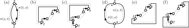
Figure 4: Since a strictly directed path from $t$ to $s$ has a lower bound for its rotation this yields upper bounds for paths from $s$ to $t$ (Lemma 1).

Lemma 1.

Let $G$ be a graph with positive flexibility and vertices $s$ and $t$ such that $G+st$ is biconnected and 4-planar. Let further $\mathcal{R}$ be a valid orthogonal representation with $s$ and $t$ incident to the common face $f$ such that $\pi_{f}(t,s)$ is strictly directed from $t$ to $s$. Then the following holds.

1. $\operatorname{rot}_{\mathcal{R}}(\pi_{f}(s,t))\leq-3$ if $f$ is the outer face and $G$ does not consist of a single path

2. $\operatorname{rot}_{\mathcal{R}}(\pi_{f}(s,t))\leq-1$ if $f$ is the outer face

3. $\operatorname{rot}_{\mathcal{R}}(\pi_{f}(s,t))\leq 5$

Proof.

We first consider the case where $f$ is the outer face (Figure 4(a)), that is cases (1) and (2). Due to the fact that $\pi_{f}(t,s)$ is strictly directed from $t$ to $s$ and the flexibility of every edge is positive, each edge on $\pi_{f}(t,s)$ has rotation at least 1. Moreover, the rotations at vertices along the path $\pi_{f}(t,s)$ are at least $-1$ since $\pi_{f}(t,s)$ is simple as $G+st$ is biconnected. Since the number of internal vertices on a path is one less than the number of edges this yields $\operatorname{rot}(\pi_{f}(t,s))\geq 1$; see Figure 4(b). If $G$ consists of a single path this directly yields $\operatorname{rot}(\pi_{f}(s,t))\leq-1$ and thus concludes case (2). For case (1) first assume that the degrees of $s$ and $t$ are not 1 (Figure 4(b)), that is $\operatorname{rot}(s_{f}),\operatorname{rot}(t_{f})\in\{-1,0,1\}$ holds. Since $f$ is the outer face the equation $\operatorname{rot}(\pi_{f}(s,t))+\operatorname{rot}(t_{f})+\operatorname{rot}(\pi_{f}(t,s))+\operatorname{rot}(s_{f})=-4$ holds and directly implies the desired inequality $\operatorname{rot}(\pi_{f}(s,t))\leq-3$. In the case that for example $t$ has degree 1 (and $\deg(s)>0$), we have $\operatorname{rot}(t_{f})=-2$ and $\operatorname{rot}(s_{f})\in\{-1,0,1\}$, thus the considerations above only yield $\operatorname{rot}(\pi_{f}(s,t))\leq-2$. However, in this case there necessarily exists a vertex $t^{\prime}$ where the paths $\pi_{f}(s,t)$ and $\pi_{f}(t,s)$ split, as illustrated in Figure 4(c). More precisely, let $t^{\prime}$ be the first vertex on $\pi_{f}(s,t)$ that also belongs to $\pi_{f}(t,s)$. Obviously, the degree of $t^{\prime}$ is at least 3 and thus $\operatorname{rot}(t^{\prime}_{f})$ (with respect to the path $\pi_{f}(t,s)$) is at least 0. Hence we obtain the stronger inequality $\operatorname{rot}(\pi_{f}(t,s))\geq 2$ yielding the desired inequality $\operatorname{rot}(\pi_{f}(s,t))\leq-3$. If $s$ and $t$ both have degree 1 we cannot only find the vertex $t^{\prime}$ but also the vertex $s^{\prime}$ where the paths $\pi_{f}(s,t)$ and $\pi_{f}(t,s)$ split. Since $G+st$ is biconnected these two vertices are distinct and the estimation above works, finally yielding $\operatorname{rot}(\pi_{f}(s,t))\leq-3$.

If $f$ is an internal face (Figure 4(d)), that is case (3) applies, we start with the equation $\operatorname{rot}(\pi_{f}(s,t))+\operatorname{rot}(t_{f})+\operatorname{rot}(\pi_{f}(t,s))+\operatorname{rot}(s_{f})=4$. First we consider the case that neither $t$ nor $s$ have degree 1. Thus, $\operatorname{rot}(t_{f}),\operatorname{rot}(s_{f})\in\{-1,0,1\}$. With the same argument as above we obtain $\operatorname{rot}(\pi_{f}(t,s))\geq 1$ and hence $\operatorname{rot}(\pi_{f}(s,t))\leq 5$; see Figure 4(e). Now assume that $t$ has degree 1 and $s$ has larger degree. Then $\operatorname{rot}(t_{f})=-2$ holds and the above estimation does not work anymore. Again, at some vertex $t^{\prime}$ the paths $\pi_{f}(t,s)$ and $\pi_{f}(s,t)$ split as illustrated in Figure 4(f). Obviously, the degree of $t^{\prime}$ needs to be greater than $2$ and thus $\operatorname{rot}(t^{\prime}_{f})$ is at least 0. This yields $\operatorname{rot}(\pi_{f}(t,s))\geq 2$ in the case that $\deg(t)=1$, compensating $\operatorname{rot}(t_{f})=-2$ (instead of $\operatorname{rot}(t_{f})\geq-1$ in the other case). To sum up, we obtain the desired inequality $\operatorname{rot}(\pi_{f}(s,t))\leq 5$. The case $\deg(s)=\deg(t)=1$ works analogously. ∎

The flex graph $G_{\mathcal{R}}^{\times}$ of $G$ with respect to a valid orthogonal representation $\mathcal{R}$ is defined to be the dual graph of $G$ such that the dual edge $e^{\star}$ is undirected if $e$ is undirected, otherwise it is directed from the face right of $e$ to the face left of $e$. Figure 5(a) shows an example graph with an orthogonal drawing together with the corresponding flex graph. Assume we have a simple directed cycle $C$ in the flex graph. Then bending along this cycle yields a new valid orthogonal representation $\mathcal{R}^{\prime}$ which is defined as follows. Let $e^{\star}=(f_{1},f_{2})$ be an edge contained in $C$ dual to $e$. Then we decrease $\operatorname{rot}(e_{f_{1}})$ and increase $\operatorname{rot}(e_{f_{2}})$ by 1. It can be easily seen that the necessary properties for $\mathcal{R}^{\prime}$ to be an orthogonal representation are satisfied. Obviously, $\operatorname{rot}_{\mathcal{R}^{\prime}}(e_{f_{1}})=-\operatorname{rot}_{\mathcal{R}^{\prime}}(e_{f_{2}})$ holds and rotations at vertices did not change. Moreover, the rotation around a face $f$ does not change since $f$ is either not contained in $C$ or it is contained in $C$, but then it has exactly one incoming and exactly one outgoing edge. Note that bending along a cycle in the flex graph preserves the planar embedding of $G$ and for every vertex the rotations in all incident faces. The following lemma shows that a high rotation along a path $\pi_{f}(s,t)$ for two vertices $s$ and $t$ sharing the face $f$ can be reduced by 1 using a directed cycle in the flex graph.

Lemma 2.

Let $G$ be a biconnected 4-planar graph with positive flexibility, a valid orthogonal representation $\mathcal{R}$ and $s$ and $t$ on a common face $f$. The flex graph $G_{\mathcal{R}}^{\times}$ contains a directed cycle $C$ such that $f\in C$, $s\in\operatorname{left}(C)$ and $t\in\operatorname{right}(C)$, if one of the following conditions holds.

1. $\operatorname{rot}_{\mathcal{R}}(\pi_{f}(s,t))\geq-2$, $f$ is the outer face and $\pi_{f}(s,t)$ is not strictly directed from $t$ to $s$

2. $\operatorname{rot}_{\mathcal{R}}(\pi_{f}(s,t))\geq 0$ and $f$ is the outer face

3. $\operatorname{rot}_{\mathcal{R}}(\pi_{f}(s,t))\geq 6$

Proof.

Figure 5(b) shows the path $\pi_{f}(s,t)$ together with the desired cycle $C$. Due to the duality of a cycle in the dual and a cut in the primal graph a directed cycle $C$ in $G_{\mathcal{R}}^{\times}$ having $s$ and $t$ to the left and to the right of $C$, respectively, induces a directed cut in $G$ that is directed from $s$ to $t$ and vice versa. Recall that directed cycles and cuts may also contain undirected edges. Assume for contradiction that such a cycle $C$ does not exist.

Claim 1.

The graph $G$ contains a strictly directed path $\pi$ from $t$ to $s$.

Every cut $(S,T)$ with $T=V\setminus S$, $s\in S$ and $t\in T$ separating $s$ from $t$ must contain an edge that is directed from $T$ to $S$, otherwise this cut would correspond to a cycle $C$ in the flex graph that does not exist by assumption. Let $T$ be the set of vertices in $G$ that can be reached by strictly directed paths from $t$. If $T$ contains $s$ we found the path $\pi$ strictly directed from $t$ to $s$. Otherwise, $(S,T)$ with $S=V\setminus T$ is a cut separating $S$ from $T$ and there cannot be an edge that is directed from a vertex in $T$ to a vertex in $S$ which is a contradiction, and thus the path $\pi$ strictly directed from $t$ to $s$ exists, which concludes the proof of the claim.

Let $G^{\prime}$ be the subgraph of $G$ induced by the paths $\pi$ and $\pi_{f}(s,t)$ together with the orthogonal representation $\mathcal{R}^{\prime}$ induced by $\mathcal{R}$.

We first consider case (1). Let $f^{\prime}$ be the outer face of the orthogonal representation $\mathcal{R}^{\prime}$. Obviously, $\pi_{f^{\prime}}(s,t)=\pi_{f}(s,t)$ and $\pi=\pi_{f^{\prime}}(t,s)$ holds, see Figure 5(c). Moreover, the graph $G^{\prime}+st$ is biconnected and $G^{\prime}$ does not consist of a single path since $\pi_{f^{\prime}}(s,t)$ and $\pi_{f^{\prime}}(t,s)$ are different due to the assumption that $\pi_{f}(s,t)$ is not strictly directed from $t$ to $s$. Since $\pi_{f^{\prime}}(t,s)$ is strictly directed from $t$ to $s$ we can use Lemma 1(1) yielding $\operatorname{rot}_{\mathcal{R}^{\prime}}(\pi_{f^{\prime}}(s,t))\leq-3$ and thus $\operatorname{rot}_{\mathcal{R}}(\pi_{f}(s,t))\leq-3$, which is a contradiction.

For case (2) exactly the same argument holds except for the case where the strictly directed path $\pi$ is the path $\pi_{f}(s,t)$ strictly directed from $t$ to $s$. In this case we have to use Lemma 1(2) instead of Lemma 1(1) yielding $\operatorname{rot}_{\mathcal{R}}(\pi_{f}(s,t))\leq-1$, which is again a contradiction.

In case (3) the subgraph $G^{\prime}$ of $G$ induced by the two paths $\pi$ and $\pi_{f}(s,t)$ again contains $s$ and $t$ on a common face $f^{\prime}$, which may be the outer or an inner face, see Figure 5(c) and Figure 5(d), respectively. In both cases we obtain $\operatorname{rot}_{\mathcal{R}}(\pi_{f}(s,t))\leq 5$ due to Lemma 1(3), which is a contradiction. ∎

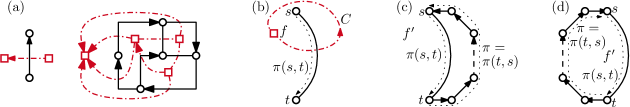
Figure 5: (a) An orthogonal representation and the corresponding flex graph where every edge has flexibility 1. (b, c, d) Illustration of Lemma 2.

Lemma 2 directly yields the following corollary, showing that graphs with positive flexibility behave very similar to single edges with positive flexibility.

Corollary 1.

Let $G$ be a graph with positive flexibility and vertices $s$ and $t$ such that $G+st$ is biconnected and 4-planar. Let further $\mathcal{R}$ be a valid orthogonal representation with $s$ and $t$ on the outer face $f$ such that $\rho=\operatorname{rot}_{\mathcal{R}}(\pi_{f}(s,t))\geq 0$. For every rotation $\rho^{\prime}\in[-1,\rho]$ there exists a valid orthogonal representation $\mathcal{R}^{\prime}$ with $\operatorname{rot}_{\mathcal{R}^{\prime}}(\pi_{f}(s,t))=\rho^{\prime}$.

Proof.

For the case that $G$ itself is biconnected, the claim follows directly from Lemma 2(2), since we can reduce the rotation along $\pi_{f}(s,t)$ stepwise by 1, starting with the orthogonal representation $\mathcal{R}$, until we reach a rotation of $-1$. For the case that $G$ itself is not biconnected we add the edge $\{s,t\}$ to the orthogonal representation $\mathcal{R}$ such that the path $\pi_{f}(s,t)$ does not change, that is $\pi_{f}(t,s)$ consists of the new edge $\{s,t\}$. Again Lemma 2(2) can be used to reduce the rotation stepwise down to $-1$. ∎

As edges with many bends imply the existence of paths with high rotation, we can use Lemma 2 to successively reduce the number of bends of every edge down to three, except for a single edge on the outer face. Since we only bend along cycles in the flex graph, neither the embedding nor the angles around vertices are changed.

Theorem 2.

Let $G$ be a biconnected 4-planar graph with positive flexibility, having a valid orthogonal representation. Then $G$ has a valid orthogonal representation with the same planar embedding, the same angles around vertices and at most three bends per edge, except for at most one edge on the outer face with up to five bends.

Proof.

In the following we essentially pick an edge with more than three bends, reduce the number of bends by one and continue with the next edge. After each of these reduction steps we set the flexibility of every edge down to $\max\{\rho,1\}$, where $\rho$ is the number of bends it currently has. This ensures that in the next step the number of bends of each edge either is decreased, remains as it is or is increased from zero to one.

We start with an edge $e=\{s,t\}$ that is incident to two faces $f_{1}$ and $f_{2}$ and has more than three bends. Due to the fact that we traverse inner faces in clockwise and the outer face in counter-clockwise direction, the edge $e$ forms in one of the two faces the path from $s$ to $t$ and in the other face the path from $t$ to $s$. Assume without loss of generality that $\pi_{f_{1}}(t,s)$ and $\pi_{f_{2}}(s,t)$ are the paths on the boundary of $f_{1}$ and $f_{2}$, respectively, that consist of $e$. Note that $\operatorname{rot}(\pi_{f_{1}}(t,s))=-\operatorname{rot}(\pi_{f_{2}}(s,t))$ holds and we assume that $\operatorname{rot}(\pi_{f_{1}}(t,s))$ is not positive. As $e$ was assumed to have more than three bends, the inequality $\operatorname{rot}(\pi_{f_{1}}(t,s))\leq-4$ holds. We distinguish between the two cases that $f_{1}$ is an inner or the outer face. We first consider the case that $f_{1}$ is an inner face; Figure 6(a) illustrates this situation for the case where $e$ has four bends. Then the rotations around the face $f_{1}$ sum up to 4. As the rotations at the vertices $s$ and $t$ can be at most 1, we obtain $\operatorname{rot}(\pi_{f_{1}}(s,t))\geq 6$. Thus we can apply Lemma 2(3) to reduce the rotation of $\pi_{f_{1}}(s,t)$ by bending along a cycle in the flex graph that contains $f_{1}$ and separates $s$ from $t$. Obviously, this increases the rotation along $\pi_{f_{1}}(t,s)$ by 1 and thus reduces the number of bends of $e$ by 1.

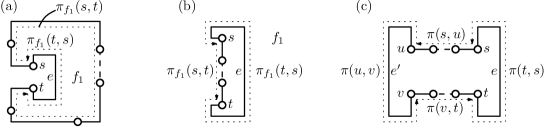
Figure 6: Reducing the number of bends on edges (Theorem 2)

For the case that $f_{1}$ is the outer face we first ignore the case where $e$ has four or five bends and show how to reduce the number of bends to five; Figure 6(b) shows the case where $e$ has six bends. Thus the inequality $\operatorname{rot}(\pi_{f_{1}}(t,s))\leq-6$ holds. As the rotations around the outer face $f_{1}$ sum up to $-4$ and the rotations at the vertices $s$ and $t$ are at most 1, the rotation along $\pi_{f_{1}}(s,t)$ must be at least 0. Thus we can apply Lemma 2(2) to reduce the rotation of $\pi_{f_{1}}(s,t)$ by 1, increasing the rotation along $\pi_{f_{1}}(t,s)$, and thus reducing the number of bends of $e$ by one.

Finally, we obtain an orthogonal representation having at most three bends per edge except for some edges on the outer face with four or five bends having their negative rotation in the outer face. If there is only one of these edges left we are done. Otherwise let $e=\{s,t\}$ be one of the edges with $\operatorname{rot}(\pi_{f}(t,s))\in\{-5,-4\}$, where $f$ is the outer face. Then the inequality $\operatorname{rot}(\pi_{f}(s,t))\geq-2$ holds by the same argument as before and we can apply Lemma 2(1) to reduce the rotation, if we can ensure that $\pi_{f}(s,t)$ is not strictly directed from $t$ to $s$. To show that, we make use of the fact that $\pi_{f}(s,t)$ contains an edge $e^{\prime}=\{u,v\}$ with at least four bends due to the assumption that $e$ was not the only edge with more than three bends. Assume without loss of generality that $u$ occurs before $v$ on $\pi_{f}(s,t)$, thus $\pi_{f}(s,t)$ splits into the three parts $\pi_{f}(s,u)$, $\pi_{f}(u,v)$ and $\pi_{f}(v,t)$. Recall that $\operatorname{rot}(\pi_{f}(s,t))\geq-2$ holds and thus $\operatorname{rot}(\pi_{f}(s,u))+\operatorname{rot}(u)+\operatorname{rot}(\pi_{f}(u,v))+\operatorname{rot}(v)+\operatorname{rot}(\pi_{f}(v,t))\geq-2$. As the rotation at the vertices $u$ and $v$ is at most 1 and the rotation of $\pi_{f}(u,v)$ at most $-4$ it follows that $\operatorname{rot}(\pi_{f}(s,u))+\operatorname{rot}(\pi_{f}(v,t))\geq 0$. Figure 6(c) illustrates the situation for the case where $e$ and $e^{\prime}$ have four bends and $\operatorname{rot}(\pi_{f}(s,u))=\operatorname{rot}(\pi_{f}(v,t))=0$. Note that at least one of the two paths is not degenerate in the sense that $s\not=u$ or $v\not=t$, otherwise the total rotation around the outer face would be at most $-6$, which is a contradiction. Assume without loss of generality that $\operatorname{rot}(\pi_{f}(s,u))\geq 0$. It follows that $\pi_{f}(s,u)$ cannot be strictly directed from $u$ to $s$ and since $\pi_{f}(s,u)$ is a subpath of $\pi_{f}(s,t)$ the path $\pi_{f}(s,t)$ cannot be strictly directed from $t$ to $s$. This finally shows that we can use part (1) of Lemma 2 implying that we can find a valid orthogonal representation such that at most a single edge with four or five bends remains, whereas all other edges have at most three bends. ∎

If we allow the embedding to be changed slightly, we obtain an even stronger result. Assume the edge $e$ lying on the outer face has more than three bends. If $e$ has five bends, we can reroute it in the opposite direction around the rest of the graph, that is we can choose the internal face incident to $e$ to be the new outer face. In the resulting drawing $e$ has obviously only three bends. Thus the following result directly follows from Theorem 2.

Corollary 2.

Let $G$ be a biconnected 4-planar graph with positive flexibility having a valid orthogonal representation. Then $G$ has a valid orthogonal representation with at most three bends per edge except for possibly a single edge on the outer face with four bends.

Note that Corollary 2 is restricted to biconnected graphs. For general graphs it implies that each block contains at most a single edge with up to four bends. Figure 7 illustrates an instance of FlexDraw with linearly many blocks and linearly many edges that are required to have four bends, showing that Corollary 2 is tight.

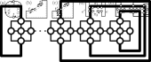
Figure 7: An instance of FlexDraw requireing linearly many edges to have four bends. Flexibilites are 1 except for the thick edges with flexibility 4.

Theorem 2 implies that it is sufficient to consider the flexibility of every edge to be at most 5, or in terms of costs we want to optimize, it is sufficient to store the cost function of an edge only in the interval $[0,5]$. However, there are two reasons why we need a stronger result. First, we want to compute cost functions of split components and thus we have to limit the number of “bends” they can have (see the next section for a precise definition of bends for split components). Second, as mentioned in the introduction (see Figure 1) the cost function of a split component may already be non-convex on the interval $[0,5]$. Fortunately, the second reason is not really a problem since there may be at most a single edge with up to five bends, all remaining edges have at most three bends and thus we only need to consider their cost functions on the interval $[0,3]$.

In the following section we focus on dealing with the first problem and strengthen the results so far presented by extending the limitation on the number of bends to split components. Note that a split pair inside an inner face of $G$ with a split component $H$ having a rotation less than $-3$ on its outer face implies a rotation of at least 6 in some inner face of $G$. Thus, we can again apply Lemma 2(3) to reduce the rotation showing that split components and single edges can be handled similarly. However, by reducing the rotation for one split component, we cannot avoid that the rotation of some other split component is increased. For single edges we did that by reducing the flexibility to the current number of bends. In the following section we extend this technique by defining a flexibility not only for edges but also for split components. We essentially show that all results we presented so far still apply, if we allow this kind of extended flexibilities.

4 Flexibility of Split Components and Nice Drawings

Let $G$ be a biconnected 4-planar graph with SPQR-tree $\mathcal{T}$ and let $\mathcal{T}$ be rooted at some node $\tau$. Recall that we do not require $\tau$ to be a Q-node. Let $\mu$ be a node of $\mathcal{T}$ that is not the root $\tau$. Then $\mu$ has a unique parent and $\operatorname{skel}(\mu)$ contains a unique virtual edge $\varepsilon=\{s,t\}$ that is associated with this parent. We call the split-pair $\{s,t\}$ a principal split pair and the pertinent graph $\operatorname{pert}(\mu)$ with respect to the chosen root a principal split component. The vertices $s$ and $t$ are the poles of this split component. Note that a single edge is also a principal split component except for the case that its Q-node is chosen to be the root. A planar embedding of $G$ is represented by $\mathcal{T}$ with the root $\tau$ if the embedding of each skeleton has the edge associated with the parent on the outer face.

Let $\mathcal{R}$ be a valid orthogonal representation of $G$ such that the planar embedding of $\mathcal{R}$ is represented by $\mathcal{T}$ rooted at $\tau$. Consider a principal split component $H$ with respect to the split pair $\{s,t\}$ and let $\mathcal{S}$ be the orthogonal representation of $H$ induced by $\mathcal{R}$. Note that the poles $s$ and $t$ are on the outer face $f$ of $\mathcal{S}$. We define $\max\{|\operatorname{rot}_{\mathcal{S}}(\pi_{f}(s,t))|,|\operatorname{rot}_{\mathcal{S}}(\pi_{f}(t,s))|\}$ to be the number of bends of the split component $H$. Note that this is a straightforward extension of the term bends as it is used for edges. With this terminology we can assign a flexibility $\operatorname{flex}(H)$ to a principal split component $H$ and we define the orthogonal representation $\mathcal{R}$ of $G$ to be valid if and only if $H$ has at most $\operatorname{flex}(H)$ bends. We say that the graph $G$ has positive flexibility if the flexibility of every principal split component is at least 1, which is straightforward extension of the original notion.

We define a valid orthogonal representation of $G$ to be nice if it is tight and if there is a root $\tau$ of the SPQR-tree such that every principal split component has at most three bends and the edge corresponding to $\tau$ in the case that $\tau$ is a Q-node has at most five bends. The main result of this section will be the following theorem, which directly extends Theorem 2.

Theorem 3.

Every biconnected 4-planar graph with positive flexibility having a valid orthogonal representation has an orthogonal representation with the same planar embedding and the same angles around vertices that is nice with respect to at least one node chosen as root of its SPQR-tree.

Before we prove Theorem 3 we need to make some additional considerations. In particular we need to extend the flex-graph such that it takes the flexibilities of principal split components into account. The extended version of the flex graph can then be used to obtain a result similar to Lemma 2, which was the main tool to proof Theorem 2. Another difficulty is that it depends on the chosen root which split components are principal split components. For the moment we avoid this problem by choosing an arbitrary Q-node to be the root of the SPQR-tree $\mathcal{T}$. Thus we only have to care about the flexibilities of the principal split components with respect to the chosen root. One might hope that the considerations we make for the flex-graph in the case of a fixed root still work, if we consider the principal split components with respect to all possible roots at the same time. However, this fails as we will see later, making it necessary to consider internal vertices as the root.

Assume that the SPQR-tree $\mathcal{T}$ of $G$ is rooted at the Q-node corresponding to an arbitrary chosen edge. Let $H$ be a principal split component with respect to the chosen root with the poles $s$ and $t$. In the embedding of $G$ the outer face $f$ of $H$ splits into two faces $f_{1}$ and $f_{2}$, where the path $\pi_{f}(s,t)$ is assumed to lie in $f_{1}$ and $\pi_{f}(t,s)$ is assumed to lie in $f_{2}$, that is $\pi_{f_{1}}(s,t)=\pi_{f}(s,t)$ and $\pi_{f_{2}}(t,s)=\pi_{f}(t,s)$. We augment $G$ by inserting the edge $\{s,t\}$ twice, embedding one of them in $f_{1}$ and the other in $f_{2}$. We denote the edge $\{s,t\}$ inserted into the face $f_{1}$ by $e_{H}(s,t)$ and the edge inserted into $f_{2}$ by $e_{H}(t,s)$. Figure 8 illustrates this process and shows how the dual graph of $G$ changes. We call the new edges $e_{H}(s,t)$ and $e_{H}(t,s)$ safety edges and define the extended flex graph $G^{\times}$ as before, ignoring that some edges have a special meaning. To simplify notation we often use the term flex graph, although we refer to the extended flex graph. Note that every cycle in the flex graph that separates $s$ from $t$ and thus crosses $\pi(s,t)$ and $\pi(t,s)$ needs to also cross the safety edges $e_{H}(s,t)$ and $e_{H}(t,s)$. Thus we can use the safety edges to ensure that the flex graph respects the flexibility of $H$ by orienting them if necessary. More precisely, we orient the safety edge $e_{H}(s,t)$ from $t$ to $s$ if $\operatorname{rot}(\pi(s,t))=-\operatorname{flex}(H)$ and similarly $e_{H}(t,s)$ from $s$ to $t$ if $\operatorname{rot}(\pi(t,s))=-\operatorname{flex}(H)$. This ensures that the rotations along $\pi(s,t)$ and $\pi(t,s)$ cannot be reduced below $-\operatorname{flex}(H)$ by bending along a cycle in the flex graph. Moreover, $\operatorname{rot}(\pi(s,t))$ cannot be increased above $\operatorname{flex}(H)$ as otherwise $\operatorname{rot}(\pi(t,s))$ has to be below $-\operatorname{flex}(H)$ and vice versa. To sum up, we insert the safety edges next to the principal split component $H$ and orient them if necessary to ensure that bending along a cycle in the flex graph respects not only the flexibilities of single edges but also the flexibility of the principal split component $H$.

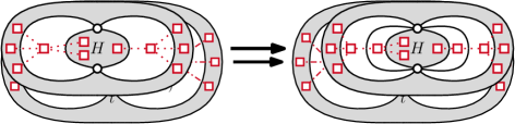
Figure 8: Augmentation of $G$ by the safety edges $e_{H}(s,t)$ and $e_{H}(t,s)$.

Since adding the safety edges for the graph $H$ is just a technique to respect the flexibility of $H$ by bending along a cycle in the flex graph, we do not draw them. Note that the augmented graph does not have maximum degree 4 anymore but this is not a problem since we do not draw the safety edges. However, we formally assign an orthogonal representation to the safety edges by essentially giving them the shape of the paths they “supervise”. More precisely, the edges $e_{H}(s,t)$ and $e_{H}(t,s)$ have the same rotations as the paths $\pi(s,t)$ and $\pi(t,s)$ on the outer face of $H$, respectively. Moreover, the angles at the vertices $s$ and $t$ are also assumed to be the same as for these two paths.

As we do not only want to respect the flexibility of a single split component, we add the safety edges for each of the principal split components at the same time. Note that the augmented graph remains planar as we only add the safety edges for the principal split components with respect to a single root. It follows directly that the considerations above still work, which would fail if the augmented graph was non-planar. This is the reason why we cannot consider the principal split components with respect to all roots at the same time. The following lemma directly extends Lemma 2 to the case where the extended flex graph is considered.

Lemma 3.

Let $G$ be a biconnected 4-planar graph with positive flexibility, a valid orthogonal representation $\mathcal{R}$ and $s$ and $t$ on a common face $f$. The extended flex graph $G_{\mathcal{R}}^{\times}$ contains a directed cycle $C$ such that $f\in C$, $s\in\operatorname{left}(C)$ and $t\in\operatorname{right}(C)$, if one of the following conditions holds.

1. $\operatorname{rot}_{\mathcal{R}}(\pi_{f}(s,t))\geq-2$, $f$ is the outer face and $\pi_{f}(s,t)$ is not strictly directed from $t$ to $s$

2. $\operatorname{rot}_{\mathcal{R}}(\pi_{f}(s,t))\geq 0$ and $f$ is the outer face

3. $\operatorname{rot}_{\mathcal{R}}(\pi_{f}(s,t))\geq 6$

Proof.

As in the proof of Lemma 2 we assume for contradiction that the cycle $C$ does not exists, yielding a strictly directed path from $t$ to $s$ in $G$. This directly yields the claim, if we can apply Lemma 1 as before. The only difference to the situation before is that the directed path from $t$ to $s$ may contain some of the safety edges. However, by definition a safety edge $e_{H}(u,v)$ is directed from $v$ to $u$ if and only if $\operatorname{rot}(\pi(u,v))=-\operatorname{flex}(H)$. As $\operatorname{flex}(H)$ is positive $\operatorname{rot}(\pi(u,v))$ has to be negative and thus the rotation along $e_{H}(u,v)$ when traversing it from $v$ to $u$ is at least 1. Thus, it does not make a difference whether the directed path from $t$ to $s$ consists of normal edges or may contain safety edges. Hence, Lemma 1 extends to the augmented graph containing the safety edges, which concludes the proof. ∎

Now we are ready to prove Theorem 3. To improve readability we state it again.

Theorem 0.

Every biconnected 4-planar graph with positive flexibility having a valid orthogonal representation has an orthogonal representation with the same planar embedding and the same angles around vertices that is nice with respect to at least one node chosen as root of its SPQR-tree.

Proof.

Let $\mathcal{R}$ be a valid orthogonal representation of $G$. We assume without loss of generality that $\mathcal{R}$ is tight. Since the operations we apply to $\mathcal{R}$ in the following do not affect the angles around vertices, the resulting orthogonal representation is also tight. Thus it remains to enforce the more interesting condition for orthogonal representations to be nice, that is reduce the number of bends of principal split components down to three. As mentioned before, the SPQR-tree $\mathcal{T}$ of $G$ is initially rooted at an arbitrary Q-node. Let $e_{\mathrm{ref}}$ be the corresponding edge. As in the proof of Theorem 2 we start with an arbitrary principal split component $H$ with more than three bends. Then one of the two paths in the outer face of $H$ has rotation less than $-3$ and we have the same situation as for a single edge, that is we can apply Lemma 3 to reduce the rotation of the opposite site and thus reduce the number of bends of $H$ by one. Afterwards, we can set the flexibility of $H$ down to the new number of bends ensuring that it is not increased later on. However, this only works if the negative rotation of the split component $H$ lies in an inner face of $G$. On the outer face we can only increase to a rotation of $-5$ yielding an orthogonal representation such that every principal split component has at most three bends, or maybe four or five bends, if it has its negative rotation in the outer face. Note that this is essentially the same situation we also had in the proof of Theorem 2. In the following we show similarly that the number of bends can be reduced further, until either a unique innermost principal split component (where innermost means minimal with respect to inclusion) or the reference edge $e_{\mathrm{ref}}$ may have more than three bends.

First assume that $e_{\mathrm{ref}}$ has more than three, that is four or five, bends and that there is a principal split component $H$ with more than three bends having its negative rotation on the outer face. Let $\{s,t\}$ be the corresponding split pair and let without loss of generality $\pi_{f}(t,s)$ be the path along $H$ with rotation less than $-3$ where $f$ is the outer face. Then the path $\pi_{f}(s,t)$ contains the edge $e_{\mathrm{ref}}=\{u,v\}$, otherwise $H$ would not be a principal split component. Moreover, $\operatorname{rot}(\pi_{f}(t,s))\leq-4$ implies that $\operatorname{rot}(\pi_{f}(s,t))\geq-2$ holds. As in the proof of Theorem 2 (compare with Figure 6(c)) the path $\pi_{f}(s,t)$ splits into the paths $\pi_{f}(s,u)$, $\pi_{f}(u,v)$ and $\pi_{f}(v,t)$. Since $\pi_{f}(u,v)$ consists of the single edge $e_{\mathrm{ref}}$ with more than three bends $\operatorname{rot}(\pi_{f}(u,v))\leq-4$ holds, implying that the rotation along $\pi_{f}(s,u)$ or $\pi_{f}(v,t)$ is greater or equal to 0. This shows that $\pi_{f}(s,t)$ cannot be strictly directed from $t$ to $s$ and thus we can apply Lemma 3(1) to reduce the number of bends $H$ has. Finally, there is no principal split component with more than three bends left and the reference edge $e_{\mathrm{ref}}$ has at most five bends, which concludes this case.

In the second case, $e_{\mathrm{ref}}$ has at most three bends. We show that if there is more than one principal split component with more than three bends, then they hierarchically contain each other. Assume that the number of bends of no principal split component that has more than three bends can be reduced further. Assume further there are two principal split components $H_{1}$ and $H_{2}$ with respect to the split pairs $\{s_{1},t_{1}\}$ and $\{s_{2},t_{2}\}$ that do not contain each other, that is without loss of generality the vertices $t_{1},s_{1},t_{2}$ and $s_{2}$ occur in this order around the outer face $f$ when traversing it in counter-clockwise direction and $\pi_{f}(t_{1},s_{1})$ and $\pi_{f}(t_{2},s_{2})$ belong to $H_{1}$ and $H_{2}$ respectively. Analogous to the case where $e_{\mathrm{ref}}$ has more than three bends we can show that Lemma 3(1) can be applied to reduce the number of bends of $H_{1}$, which is a contradiction. Thus, either $H_{1}$ is contained in $H_{2}$ or the other way round. This shows that there is a unique principal split component $H$ that is minimal with respect to inclusion having more than three bends. Due to the inclusion property, all nodes in the SPQR-tree corresponding to the principal split components with more than three bends lie on the path between the current root and the node corresponding to $H$. We denote the node corresponding to $H$ by $\tau$ and choose $\tau$ to be the new root of the SPQR-tree $\mathcal{T}$. Since the principal split components depend on the root chosen for $\mathcal{T}$ some split components may no longer be principal and some may become principal due to rerooting. Our claim is that all principal split components with more than three bends are no longer principal after rerooting and furthermore that all split components becoming principal can be enforced to have at most three bends.

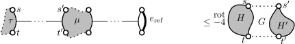
Figure 9: The path between the new and the old root in the SPQR-tree containing $\mu$ (left). The whole graph $G$ containing the principal split component $H^{\prime}$ corresponding to $\mu$ with respect to the new root and the principal split component $H$ of the new root with respect to the old root (right).

First note that the principal split component corresponding to a node $\mu$ in the SPQR-tree changes if and only if $\mu$ lies on the path between the old and the new root, that is between $\tau$ and the Q-node corresponding to $e_{\mathrm{ref}}$. Since all principal split components (with respect to the old root) that have more than three bends also lie on this path, all these split components are no longer principal (with respect to the new root). It remains to deal with the new principal split components corresponding to the nodes on this path. Note that the new root $\tau$ itself has no principal split component associated with it. Let $\mu\not=\tau$ be a node on the path between the new and the old root and let $H^{\prime}$ be the new principal split component corresponding to $\mu$ with the poles $s^{\prime}$ and $t^{\prime}$. Recall that $H$ is the former principal split component corresponding to the new root $\tau$ with the poles $s$ and $t$. Note that $H$ of course is still a split component, although it is not principal anymore. Figure 9 illustrates this situation. Now assume that $H^{\prime}$ has more than three bends. Then there are two possibilities, either it has its negative rotation on the outer face or in some inner face. If only the latter case arises we can easily reduce the number of bends down to three as we did before. In the remaining part of the proof we show that the former case cannot arise due to the assumption that the number of bends of $H$ cannot be reduced anymore. Assume $H^{\prime}$ has its negative rotation in the outer face $f$, that is without loss of generality the path $\pi_{f}(t,s)$ belongs to $H^{\prime}$ and has rotation at most $-4$. Thus we have again the situation that the two split components $H^{\prime}$ and $H$ both have a rotation of at most $-4$ in the outer face. Moreover, these two split components do not contain or overlap each other since $s$ and $t$ are not contained in $H^{\prime}$ as $\tau$ is the new root and $H$ does not contain $s^{\prime}$ or $t^{\prime}$ since $\mu$ is an ancestor of $\tau$ with respect to the old root. Thus we could have reduced the number of bends of $H$ before we changed the root, which is a contradiction to the assumption we made that the number of bends of principal split components with more than three bends cannot be reduced anymore. Hence, all new principal split components either have at most three bends or they have their negative rotation in some inner face. Finally, we obtain a valid orthogonal representation with at most three bends per principal split component with respect to $\tau$. ∎

5 Optimal Drawings with Fixed Planar Embedding

All results from the previous sections deal with the case where we are only interested in the decision problem of whether a given graph has a valid drawing or not. More precisely, we always assumed to have a valid orthogonal representation of an instance of FlexDraw and showed that this implies that there exists another valid orthogonal representation with certain properties. In this section, we consider convex instances of the optimization problem OptimalFlexDraw. The following generic theorem shows that the results for FlexDraw that we presented so far can be extended to OptimalFlexDraw.

Theorem 4.

If the existence of a valid orthogonal representation of an instance of FlexDraw with positive flexibility implies the existence of a valid orthogonal representation with property $P$, then every convex instance of OptimalFlexDraw has an optimal drawing with property $P$.

Proof.

Let $G$ be a convex instance of OptimalFlexDraw. Let further $\mathcal{R}$ be an optimal orthogonal representation. We can reinterpret $G$ as an instance of FlexDraw with positive flexibility by setting the flexibility of an edge with $\rho$ bends in $\mathcal{R}$ to $\max\{\rho,1\}$. Then $\mathcal{R}$ is obviously a valid orthogonal representation of $G$ with respect to these flexibilities. Thus there exists another valid orthogonal representation $\mathcal{R}^{\prime}$ having property $P$. It remains to show that $\operatorname{cost}(\mathcal{R}^{\prime})\leq\operatorname{cost}(\mathcal{R})$ holds when going back to the optimization problem OptimalFlexDraw. However, this is clear for the following reason. Every edge $e$ has as most as many bends in $\mathcal{R}^{\prime}$ as in $\mathcal{R}$ except for the case where $e$ has one bend in $\mathcal{R}^{\prime}$ and zero bends in $\mathcal{R}$. In the former case the monotony of $\operatorname{cost}_{e}(\cdot)$ implies that the cost did not increase. In the latter case $e$ causes the same amount of cost in $\mathcal{R}$ as in $\mathcal{R}^{\prime}$ since $\operatorname{cost}_{e}(0)=\operatorname{cost}_{e}(1)=b_{e}$ holds for convex instances of OptimalFlexDraw. Note that this proof still works, if the cost functions are only monotone but not convex. ∎

It follows that every convex 4-planar graph has an optimal drawing that is nice since Theorem 4 shows that Theorem 3 can be applied. Thus, it is sufficient to consider only nice drawings when searching for an optimal solution, as there exists a nice optimal solution. This is a fact that we crucially exploit in the next section since although the cost function of a principal split component may be non-convex, we can show that it is convex in the interval that is of interest when only considering nice drawings.

6 Optimal Drawings with Variable Planar Embedding

All results we presented so far were based on a fixed planar embedding of the input graph $G$. In this section we present an algorithm that computes an optimal drawing of $G$ in polynomial time, optimizing over all planar embeddings of $G$. Our algorithm crucially relies on the existence of a nice drawing among all optimal drawings of $G$. For biconnected graphs (Section 6.1) we present a dynamic program that computes the cost function of all principal split components bottom-up in the SPQR-tree with respect to a chosen root. To compute the optimal drawing among all drawings that are nice with respect to the chosen root, it remains to consider the embeddings of the root itself. If we choose every node to be the root once, this directly yields an optimal drawing of $G$ taking all planar embeddings into account. In Section 6.2 we extend our results to connected graphs that are not necessarily biconnected. To this end we first modify the algorithm for biconnected graphs such that it can compute an optimal drawing with the additional requirement that a specific vertex lies on the outer face. Then we can use the BC-tree to solve OptimalFlexDraw for connected graphs. We use the computation of a minimum-cost flow in a network of size $n$ as a subroutine and denote the consumed running time by $T_{\operatorname{flow}}(n)$. In Section 6.3 we consider which running time we actually need.

6.1 Biconnected Graphs

In this section we always assume $G$ to be a biconnected 4-planar graph forming a convex instance of OptimalFlexDraw. Let $\mathcal{T}$ be the SPQR-tree of $G$. As defined before, an orthogonal representation is optimal if it has the smallest possible cost. We call an orthogonal representation $\tau$-optimal if it has the smallest possible cost among all orthogonal representation that are nice with respect to the root $\tau$. We say that it is $(\tau,\mathcal{E})$-optimal if it causes the smallest possible amount of cost among all orthogonal representations that are nice with respect to $\tau$ and induce the planar embedding $\mathcal{E}$ on $\operatorname{skel}(\tau)$. In this section we concentrate on finding a $(\tau,\mathcal{E})$-optimal orthogonal representation with respect to a root $\tau$ and a given planar embedding $\mathcal{E}$ of $\operatorname{skel}(\tau)$. Then a $\tau$-optimal representation can be computed by choosing every possible embedding of $\operatorname{skel}(\tau)$. An optimal solution can then be computed by choosing every node in $\mathcal{T}$ to be the root once.

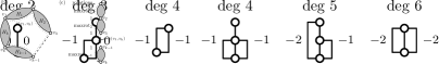
Figure 10: Split components with as few bends as possible.

In Section 4 we extended the terms “bends” and “flexibility”, which were originally defined for single edges, to arbitrary principal split components with respect to the chosen root. We start out by making precise what we mean with the cost function $\operatorname{cost}_{H}(\cdot)$ of a principal split component $H$ with poles $s$ and $t$. Recall that the number of bends of $H$ with respect to an orthogonal representation $\mathcal{S}$ with $s$ and $t$ on the outer face $f$ is defined to be $\max\{|\operatorname{rot}_{\mathcal{S}}(\pi_{f}(s,t))|,|\operatorname{rot}_{\mathcal{S}}(\pi_{f}(t,s))|\}$. Assume $\mathcal{S}$ is the nice orthogonal representation of $H$ that has the smallest possible cost among all nice orthogonal representations with $\rho$ bends. Then we essentially define $\operatorname{cost}_{H}(\rho)$ to be the cost of $\mathcal{S}$. However, with this definition the cost function of $H$ is not defined for all $\rho\in\mathbb{N}_{0}$ since $H$ does not have an orthogonal representation with zero bends at all, if $\deg(s)>1$ or $\deg(t)>1$, as at least one of the paths $\pi_{f}(s,t)$ and $\pi_{f}(t,s)$ has negative rotation in this case. More precisely, if $\deg(s)+\deg(t)>2$, then $H$ has at least one bend, and if $\deg(s)+\deg(t)>4$, then $H$ has at least two bends. Figure 10 shows for each combination of degrees a small example with the smallest possible number of bends. In these two cases we formally set $\operatorname{cost}_{H}(0)=\operatorname{cost}_{H}(1)$ and $\operatorname{cost}_{H}(0),\operatorname{cost}_{H}(1)=\operatorname{cost}_{H}(2)$, respectively. Thus, we only need to compute the cost functions for at least $\lceil(\deg(s)+\deg(t)-2)/2\rceil$ bends. We denote this lower bound by $\ell_{H}=\lceil(\deg(s)+\deg(t)-2)/2\rceil$. Hence, it remains to compute the cost function $\operatorname{cost}_{H}(\rho)$ for $\rho\in[\ell_{H},3]$. For more than three bends we formally set the cost to $\infty$. Note that the definition of the cost function only considers nice orthogonal representations (including that they are tight). As a result of this restriction the cost for an orthogonal representation with $\rho$ bends might be less than $\operatorname{cost}_{H}(\rho)$. However, due to Theorem 3 in combination with Theorem 4 we know that optimizing over nice orthogonal representations is sufficient to find an optimal solution.

As for single edges, we define the base cost $b_{H}$ of the principal split component $H$ to be $\operatorname{cost}_{H}(0)$. We will see that the cost function $\operatorname{cost}_{H}(\cdot)$ is monotone and even convex in the interval $[0,3]$ (except for a special case) and thus the base cost is the smallest possible amount of cost that has to be payed for every orthogonal drawing of $H$. The only exception is the case where $\deg(s)=\deg(t)=3$. In this case $H$ has at least two bends and thus the cost function $\operatorname{cost}_{H}(\cdot)$ needs to be considered only on the interval $[2,3]$. However, it may happen that $\operatorname{cost}_{H}(2)>\operatorname{cost}_{H}(3)$ holds in this case. Then we set the base cost $b_{H}$ to $\operatorname{cost}_{H}(3)$ such that the base cost $b_{H}$ is really the smallest possible amount of cost that need to be payed for every orthogonal representation of $H$. We obtain the following theorem.

Theorem 5.

If the poles of a principal split component do not both have degree 3, then its cost function is convex on the interval $[0,3]$.

Before showing Theorem 5 we just assume that it holds and moreover we assume that the cost function of every principal split component is already computed. We first show how these cost functions can then be used to compute an optimal drawing. To this end, we define a flow network on the skeleton of the root $\tau$ of the SPQR-tree, similar to Tamassias flow network [15]. The cost functions computed for the children of $\tau$ will be used as cost functions on arcs in the flow network. As we can only solve flow networks with convex costs we somehow have to deal with potentially non-convex cost functions for the case that both endvertices of a virtual edge have degree 3 in its expansion graph. Our strategy is to simply ignore these subgraphs by contracting them into single vertices. Note that the resulting vertices have degree 2 since the poles of graphs with non-convex cost functions have degree 3. The process of replacing the single vertex in the resulting drawing by the contracted component is illustrated in Figure 11. The following lemma justifies this strategy.

Figure 11: A single vertex can be replaced by a split component with three bends.

Lemma 4.

Let $G$ be a biconnected convex instance of OptimalFlexDraw with $\tau$-optimal orthogonal representation $\mathcal{R}$ and let $H$ be a principal split component with non-convex cost function and base cost $b_{H}$. Let further $G^{\prime}$ be the graph obtained from $G$ by contracting $H$ into a single vertex and let $\mathcal{R}^{\prime}$ be a $\tau$-optimal orthogonal representation of $G^{\prime}$. Then $\operatorname{cost}(\mathcal{R})=\operatorname{cost}(\mathcal{R}^{\prime})+b_{H}$ holds.

Proof.

Assume we have a $\tau$-optimal orthogonal representation $\mathcal{R}$ of $G$ inducing the orthogonal representation $\mathcal{S}$ on $H$. As $H$ has either two or three bends we can simply contract it yielding an orthogonal representation $\mathcal{R}^{\prime}$ of $G$ with $\operatorname{cost}(\mathcal{R}^{\prime})=\operatorname{cost}(\mathcal{R})-\operatorname{cost}(\mathcal{S})\leq\operatorname{cost}(\mathcal{R})-b_{H}$. The opposite direction is more complicated. Assume we have an orthogonal representation $\mathcal{R}^{\prime}$ of $G^{\prime}$, then we want to construct an orthogonal representation $\mathcal{R}$ of $G$ with $\operatorname{cost}(\mathcal{R})=\operatorname{cost}(\mathcal{R}^{\prime})+b_{H}$. Let $\mathcal{S}$ be an orthogonal representation of $H$ causing only $b_{H}$ cost. Since $\operatorname{cost}_{H}(\cdot)$ was assumed to be non-convex, $\mathcal{S}$ needs to have three bends. It is easy to see that $\mathcal{R}^{\prime}$ and $\mathcal{S}$ (or $\mathcal{S}^{\prime}$ obtained from $\mathcal{S}$ by mirroring the drawing) can be combined to an orthogonal representation of $G$ if the two edges incident to the vertex $v$ in $G^{\prime}$ corresponding to $H$ have an angle of $90^{\circ}$ between them. However, this can always be ensured without increasing the costs of $\mathcal{R}^{\prime}$. Let $e_{1}$ and $e_{2}$ be the edges incident to $v$ and assume they have an angle of $180^{\circ}$ between them in both faces incident to $v$. If neither $e_{1}$ nor $e_{2}$ has a bend, the flex graph contains the cycle around $v$ due to the fact that $e_{1}$ and $e_{2}$ have positive flexibilities. Bending along this cycles introduces a bend to each of the edges, thus we can assume without loss of generality that $e_{1}$ has a bend in $\mathcal{R}^{\prime}$. Moving $v$ along the edge $e_{1}$ until it reaches this bend decreases the number of bends on $e_{1}$ by one and ensures that $v$ has an angle of $90^{\circ}$ in one of its incident faces. Thus we can replace $v$ by the split component $H$ with orthogonal representation $\mathcal{S}$ having cost $b_{H}$ yielding an orthogonal representation $\mathcal{R}$ of $G$ with $\operatorname{cost}(\mathcal{R})=\operatorname{cost}(\mathcal{R}^{\prime})+b_{H}$. ∎

When computing a $(\tau,\mathcal{E})$-optimal orthogonal representation of $G$ we make use of Lemma 4 in the following way. If the expansion graph $H$ corresponding to a virtual edge $\varepsilon$ in $\operatorname{skel}(\tau)$ has a non-convex cost function, we simply contract this virtual edge in $\operatorname{skel}(\tau)$. Note that this is equivalent to contracting $H$ in $G$. We can then make use of the fact that all remaining expansion graphs have convex cost functions to compute a $(\tau,\mathcal{E})$-optimal orthogonal representation of the resulting graph yielding a $(\tau,\mathcal{E})$-optimal orthogonal representation of the original graph $G$ since the contracted expansion graphs can be inserted due to Lemma 4. Note that expansion graphs with non convex cost functions can only appear if the root is a Q- or an S-node. In the skeletons of P- and R-nodes every vertex has degree at least three, thus the poles of an expansion graph cannot have degree 3 since $G$ has maximum degree 4.

Figure 12: (a) The structure of the flow network $N^{\mathcal{E}}$ for the case that $\tau$ is an R-node with $\operatorname{skel}(\tau)=K_{4}$. The outer face is split into several gray boxes to improve readability. (b) A flow together with the corresponding orthogonal representation. The numbers indicate the amount of flow on the arcs. Undirected edges imply 0 flow, directed arcs without a number have flow 1.

Now we are ready to define the flow network $N^{\mathcal{E}}$ on $\operatorname{skel}(\tau)$ with respect to the fixed embedding $\mathcal{E}$ of $\operatorname{skel}(\tau)$; see Figure 12(a) for an example. For each vertex $v$, each virtual edge $\varepsilon$ and each face $f$ in $\operatorname{skel}(\tau)$ the flow network $N^{\mathcal{E}}$ contains the nodes $v$, $\varepsilon$ and $f$, called vertex node, edge node and face node, respectively. The network $N^{\mathcal{E}}$ contains the arcs $(v,f)$ and $(f,v)$ with capacity 1, called vertex-face arcs, if the vertex $v$ and the face $f$ are incident in $\operatorname{skel}(\tau)$. For every virtual edge $\varepsilon$ we add edge-face arcs $(\varepsilon,f)$ and $(f,\varepsilon)$, if $f$ is incident to $\varepsilon$. We use $\operatorname{cost}_{H}(\cdot)-b_{H}$ as cost function of the arc $(f,\varepsilon)$, where $H$ is the expansion graph of the virtual edge $\varepsilon$. The edge-face arcs $(\varepsilon,f)$ in the opposite direction have infinite capacity with 0 cost. It remains to define the demand of every node in $N^{\mathcal{E}}$. Every inner face has a demand of 4, the outer face has a demand of $-4$. An edge node $\varepsilon$ stemming from the edge $\varepsilon=\{s,t\}$ with expansion graph $H$ has a demand of $\deg_{H}(s)+\deg_{H}(t)-2$, where $\deg_{H}(v)$ denotes the degree of $v$ in $H$. The demand of a vertex node $v$ is $4-\deg_{G}(v)-\deg_{\operatorname{skel}(\tau)}(v)$.

In the flow network $N^{\mathcal{E}}$ the flow entering a face node $f$ using a vertex-face arc or an edge-face arc is interpreted as the rotation at the corresponding vertex or along the path between the poles of the corresponding child, respectively; see Figure 12(b) for an example. Incoming flow is positive rotation and outgoing flow negative rotation. Let $b_{H_{1}},\dots,b_{H_{k}}$ be the base costs of the expansion graphs corresponding to virtual edges in $\operatorname{skel}(\tau)$. We define the total base costs of $\tau$ to be $b_{\tau}=\sum_{i}b_{H_{i}}$. Note that the total base costs of $\tau$ are a lower bound for the costs that have to be paid for every orthogonal representation of $G$. We show that an optimal flow $\phi$ in $N^{\mathcal{E}}$ corresponds to a $(\tau,\mathcal{E})$-optimal orthogonal representation $\mathcal{R}$ of $G$. Since the base costs do not appear in the flow network, the costs of the flow and its corresponding orthogonal representation differ by the total base costs $b_{\tau}$, that is $\operatorname{cost}(\mathcal{R})=\operatorname{cost}(\phi)+b_{\tau}$. We obtain the following lemma.

Lemma 5.

Let $G$ be a biconnected convex instance of OptimalFlexDraw, let $\mathcal{T}$ be its SPQR-tree with root $\tau$ and let $\mathcal{E}$ be an embedding of $\operatorname{skel}(\tau)$. If the cost function of every principal split component is known, a $(\tau,\mathcal{E})$-optimal solution can be computed in $\mathcal{O}(T_{\operatorname{flow}}(|\operatorname{skel}(\tau)|))$ time.

Proof.

As mentioned before, we want to use the flow network $N^{\mathcal{E}}$ to compute an optimal orthogonal representation. To this end we show two directions. First, given a $(\tau,\mathcal{E})$-optimal orthogonal representation $\mathcal{R}$, we obtain a feasible flow $\phi$ in $N^{\mathcal{E}}$ such that $\operatorname{cost}(\phi)=\operatorname{cost}(\mathcal{R})-b_{\tau}$, where $b_{\tau}$ are the total base costs. Conversely, given an optimal flow $\phi$ in $N^{\mathcal{E}}$, we show how to construct an orthogonal representation $\mathcal{R}$ such that $\operatorname{cost}(\mathcal{R})=\operatorname{cost}(\phi)+b_{\tau}$. As the flow network $N^{\mathcal{E}}$ has size $\mathcal{O}(|\operatorname{skel}(\tau)|)$, the claimed running time follows immediately.

Let $\mathcal{R}$ be a $(\tau,\mathcal{E})$-optimal orthogonal representation of $G$. As we only consider nice and thus only tight drawings we can assume the orthogonal representation $\mathcal{R}$ to be tight. Recall that being tight implies that the poles of the expansion graph of every virtual edge have a rotation of 1 in the internal faces. We first show how to assign flow to the arcs in $N^{\mathcal{E}}$. It can then be shown that the resulting flow is feasible and causes $\operatorname{cost}(\mathcal{R})-b_{\tau}$ cost. For every pair of vertex-face arcs $(f,v)$ and $(v,f)$ in $N^{\mathcal{E}}$ there exists a corresponding face $f$ in the orthogonal representation $\mathcal{R}$ of $G$ and we set $\phi((v,f))=\operatorname{rot}(v_{f})$. Let $\varepsilon=\{s,t\}$ be a virtual edge in $\operatorname{skel}(\mu)$ incident to the two faces $f_{1}$ and $f_{2}$. Without loss of generality let $\pi_{f_{1}}(s,t)$ be the path belonging to the expansion graph of $\varepsilon$. Then $\pi_{f_{2}}(t,s)$ also belongs to $H$. We set $\phi((\varepsilon,f_{1}))=\operatorname{rot}_{\mathcal{R}}(\pi_{f_{1}}(s,t))$ and $\phi((\varepsilon,f_{2}))=\operatorname{rot}_{\mathcal{R}}(\pi_{f_{2}}(t,s))$. For the resulting flow $\phi$ we need to show that the capacity of every arc is respected, that the demand of every vertex is satisfied, and that $\operatorname{cost}(\phi)=\operatorname{cost}(\mathcal{R})-b_{\tau}$ holds.

First note that the flow on the vertex-face arcs does not exceed the capacities of 1 since every vertex has degree at least 2. Since no other arc has a capacity, it remains to deal with the demands and the costs.

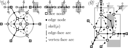
Figure 13: (a) Illustration of the demand of virtual edges. (b) Rotation of poles in the outer face, depending on the degree.

For the demands we consider each vertex type separately. Let $f$ be a face node. The total incoming flow entering $f$ is obviously equal to the rotation in $\mathcal{R}$ around the face $f$. As $\mathcal{R}$ is an orthogonal representation this rotation equals to 4 ($-4$ for the outer face), which is exactly the demand of $f$. Let $\varepsilon$ be an edge node corresponding to the expansion graph $H$ with poles $s$ and $t$. Recall that $\operatorname{dem}(\varepsilon)=\deg_{H}(s)+\deg_{H}(t)-2$ is the demand of $\varepsilon$. Figure 13(a) illustrates the demand of a virtual edge. Let $\mathcal{S}$ be the orthogonal representation induced on $H$ by $\mathcal{R}$ and let $f$ be the outer face of $\mathcal{S}$. Clearly, the flow leaving $\varepsilon$ is equal to $\operatorname{rot}_{\mathcal{R}}(\pi_{f_{1}}(s,t))+\operatorname{rot}_{\mathcal{R}}(\pi_{f_{2}}(t,s))=\operatorname{rot}_{\mathcal{S}}(\pi_{f}(s,t))+\operatorname{rot}_{\mathcal{S}}(\pi_{f}(t,s))$. Since $f$ is the outer face of $H$, the total rotation around this faces sums up to $-4$. The rotation of the pole $s$ in the outer face $f$ is $\deg_{H}(s)-3$, see Figures 13(b), and the same holds for $t$. Thus we have $\operatorname{rot}_{\mathcal{S}}(\pi_{f}(s,t))+\operatorname{rot}_{\mathcal{S}}(\pi_{f}(t,s))+\deg_{H}(s)-3+\deg_{H}(t)-3=-4$. This yields for the outgoing flow $\operatorname{rot}_{\mathcal{S}}(\pi_{f}(s,t))+\operatorname{rot}_{\mathcal{S}}(\pi_{f}(t,s))=2-\deg_{H}(s)-\deg_{H}(t)$, which is exactly the negative demand of $\varepsilon$. It remains to consider the vertex nodes. Let $v$ be a vertex node, recall that $\operatorname{dem}(v)=4-\deg_{G}(v)-\deg_{\operatorname{skel}(\tau)}(v)$ holds. The outgoing flow leaving $v$ is equal to the summed rotation of $v$ in faces not belonging to expansion graphs of virtual edges in $\operatorname{skel}(\tau)$. As $\mathcal{R}$ is an orthogonal representation, the total rotation around every vertex $v$ is $2\cdot(\deg_{G}(v)-2)$. Moreover, $v$ is incident to $\deg_{\operatorname{skel}(\tau)}(v)$ faces that are not contained in expansion graphs of virtual edges of $\operatorname{skel}(\tau)$. Thus there are $\deg_{G}(v)-\deg_{\operatorname{skel}(\tau)}(v)$ faces incident to $v$ belonging to expansion graphs. As we assumed that the orthogonal representation of every expansion graph is tight, the rotation of $v$ in each of these faces is 1. Thus the rotation of $v$ in the remaining faces not belonging to expansion graphs is $2\cdot(\deg_{G}(v)-2)-(\deg_{G}(v)-\deg_{\operatorname{skel}(\tau)}(v))$. Rearrangement yields a rotation, and thus an outgoing flow, of $\deg_{G}(v)+\deg_{\operatorname{skel}(\tau)}(v)-4$, which is the negative demand of $v$.

To show that $\operatorname{cost}(\phi)=\operatorname{cost}(\mathcal{R})-b_{\tau}$ holds it suffices to consider the flow on the edge-face arcs as no other arcs cause cost. Let $\varepsilon$ be a virtual edge and let $f_{1}$ and $f_{2}$ the two incident faces. The flow entering $f_{1}$ or $f_{2}$ does not cause any cost, as $(\varepsilon,f_{1})$ and $(\varepsilon,f_{2})$ have infinite capacity with 0 cost. Thus only flow entering $\varepsilon$ over the arcs $(f_{1},\varepsilon)$ and $(f_{2},\varepsilon)$ may cause cost. Assume without loss of generality that the number of bends $\rho$ the expansion graph $H$ of $\varepsilon$ has is determined by the rotation along $\pi_{f_{1}}(s,t)$, that is $\rho=-\operatorname{rot}_{\mathcal{R}}(\pi_{f_{1}}(s,t))$. Let $\rho^{\prime}=-\operatorname{rot}_{\mathcal{R}}(\pi_{f_{2}}(t,s))$ be the negative rotation along the path $\pi_{f_{2}}(t,s)$ in the face $f_{2}$. Note that $\phi((f_{1},\varepsilon))=\rho$ and $\phi((f_{2},\varepsilon))=\rho^{\prime}$. Obviously, the flow on $(f_{1},\varepsilon)$ causes the cost $\operatorname{cost}_{H}(\rho)-b_{H}$. We show that the cost caused by the flow on $(f_{2},\varepsilon)$ is 0. If $\rho^{\prime}\leq 0$ this is obviously true, as there is no flow on the edge $(f_{2},\varepsilon)$. Otherwise, $0<\rho^{\prime}\leq\rho$ holds. It follows that the smallest possible number of bends $\ell_{H}$ every orthogonal representation of $H$ has lies between $\rho^{\prime}$ and $\rho$. It follows from the definition of $\operatorname{cost}_{H}(\cdot)$ and from the fact that all cost functions are convex that $\operatorname{cost}_{H}(\rho^{\prime})=b_{H}$. To sum up, the total cost on edge-face arcs incident to the virtual edge $\varepsilon$ is equal to the cost caused by its expansion graph $H$ with respect to the orthogonal representation $\mathcal{R}$ minus the base cost $b_{H}$. As neither $\phi$ nor $\mathcal{R}$ have additional cost we obtain $\operatorname{cost}(\phi)=\operatorname{cost}(\mathcal{R})-b_{\tau}$.

It remains to show the opposite direction, that is given an optimal flow $\phi$ in $N^{\mathcal{E}}$, we can construct an orthogonal representation $\mathcal{R}$ of $G$ such that $\operatorname{cost}(\mathcal{R})=\operatorname{cost}(\phi)+b_{\tau}$. This can be done by reversing the construction above. The flow on edge-face arcs determines the number of bends for the expansion graphs of each virtual edge. The cost functions of these expansion graphs guarantee the existence of orthogonal representations with the desired rotations along the paths between the poles, thus we can assume to have orthogonal representations for all children. We combine these orthogonal representations by setting the rotations between them at common poles as specified by the flow on vertex-face arcs. It can be easily verified that this yields an orthogonal representation of the whole graph $G$ by applying the above computation in the opposite direction. ∎

The above results rely on the fact that the cost functions of principal split components are convex as stated in Theorem 5 and that they can be computed efficiently. In the following we show that Theorem 5 really holds with the help of a structural induction over the SPQR-tree. More precisely, the cost functions of principal split components corresponding to the leaves of $\mathcal{T}$ are the cost functions of the edges and thus they are convex. For an inner node $\mu$ we assume that the pertinent graphs of the children of $\mu$ have convex cost functions and show that $H=\operatorname{pert}(\mu)$ itself also has a convex cost function. The proof is constructive in the sense that it directly yields an algorithm to compute these cost functions bottom up in the SPQR-tree.

Note that we can again apply Lemma 4 in the case that the cost function of the expansion graph of one of the virtual edges in $\operatorname{skel}(\mu)$ is not convex due to the fact that both of its poles have degree 3. This means that we can simply contract such a virtual edge (corresponding to a contraction of the expansion graph in $H$), compute the cost function for the remaining graph instead of $H$ and plug the contracted expansion graph into the resulting orthogonal representations. Thus we can assume that the cost function of each of the expansion graphs is convex, without any exceptions.

The flow network $N^{\mathcal{E}}$ that was introduced to compute an optimal orthogonal representation in the root of the SPQR-tree can be adapted to compute the cost function of the principal split component $H$ corresponding to a non-root node $\mu$. To this end we have to deal with the parent edge, which does not occur in the root of $\mathcal{T}$, and we consider a parameterization of $N^{\mathcal{E}}$ to compute several optimal orthogonal representations with a prescribed number of bends, depending on the parameter in the flow network. Before we describe the changes in the flow network we need to make some considerations about the cost function. By the definition of the cost function it explicitely optimizes over all planar embeddings of $\operatorname{skel}(\mu)$. Moreover, as the cost function $\operatorname{cost}_{H}(\rho)$ depends on the number of bends $\rho$ a graph $H$ has, it implicitly allows to flip the embedding of $H$ since the number of bends is defined as $\max\{|\operatorname{rot}(\pi(s,t))|,|\operatorname{rot}(\pi(t,s))|\}$. However, the flow network $N^{\mathcal{E}}$ can only be used to compute the cost function for a fixed embedding. Thus we define the partial cost function $\operatorname{cost}_{H}^{\mathcal{E}}(\rho)$ of $H$ with respect to the planar embedding $\mathcal{E}$ of $\operatorname{skel}(\mu)$ to be the smallest possible cost of an orthogonal representation inducing the planar embedding $\mathcal{E}$ on $\operatorname{skel}(\mu)$ with $\rho$ bends such that the number of bends is determined by $\pi_{f}(s,t)$, that is $\operatorname{rot}(\pi_{f}(s,t))=-\rho$, where $f$ is the outer face. Note that the minimum over the partial cost functions $\operatorname{cost}_{H}^{\mathcal{E}}(\cdot)$ and $\operatorname{cost}_{H}^{\mathcal{E}^{\prime}}(\cdot)$, where $\mathcal{E}^{\prime}$ is obtained by flipping the embedding $\mathcal{E}$ of $\operatorname{skel}(\mu)$ yields a function describing the costs of $H$ with respect to the embedding $\mathcal{E}$ of $\operatorname{skel}(\mu)$ depending on the number of bends $H$ has (and not on the rotation along $\pi_{f}(s,t)$ as the partial cost function does). Obviously, minimizing over all partial cost functions yields the cost function of $H$.

The flow network $N^{\mathcal{E}}$ is defined as before with the following modifications. The parent edge of $\operatorname{skel}(\mu)$ does not have a corresponding edge node. Let $f_{1}$ and $f_{2}$ be the faces in $\operatorname{skel}(\mu)$ incident to the parent edge. These two faces together form the outer face $f$ of $H$, thus we could merge them into a single face node. However, not merging them has the advantage that the incoming flow in $f_{1}$ and $f_{2}$ corresponds to the rotations along $\pi_{f}(s,t)$ and $\pi_{f}(t,s)$, respectively (it might be the other way round but we can assume this situation without loss of generality). Thus, we do not merge $f_{1}$ and $f_{2}$, which enables us to control the number of bends of $H$ by setting the demands of $f_{1}$ and $f_{2}$. This is also the reason why we remove the vertex-face arcs between the poles and the two faces $f_{1}$ and $f_{2}$. Before we describe how to set the demands of $f_{1}$ and $f_{2}$, we fit the demands of the poles to the new situation. As we only consider tight orthogonal representations we know that the rotation at the poles $s$ and $t$ in all inner faces is 1. Thus, we set $\operatorname{dem}(s)=2-\deg_{\operatorname{skel}(\mu)}(s)$ and $\operatorname{dem}(t)=2-\deg_{\operatorname{skel}(\mu)}(t)$ as this is the number of faces incident to $s$ and $t$, respectively, after removing the vertex-face arcs to $f_{1}$ and $f_{2}$. With these modifications the only flow entering $f_{1}$ and $f_{2}$ comes from the paths $\pi_{f}(s,t)$ and $\pi_{f}(t,s)$, respectively. As the total rotation around the outer face is $-4$ and the rotation at the vertices $s$ and $t$ is $\deg_{H}(s)-3$ and $\deg_{H}(t)-3$, respectively, we have to ensure that $\operatorname{dem}(f_{1})+\operatorname{dem}(f_{2})=2-\deg_{H}(s)-\deg_{H}(t)$. As mentioned before, we assume without loss of generality that $\pi_{f}(s,t)$ belongs to the face $f_{1}$ and $\pi_{f}(t,s)$ belongs to $f_{2}$. Then the incoming flow entering $f_{1}$ corresponds to $\operatorname{rot}(\pi_{f}(s,t))$ of an orthogonal representation. We parameterize $N^{\mathcal{E}}$ with respect to the faces $f_{1}$ and $f_{2}$ starting with $\operatorname{dem}(f_{1})=0$ and $\operatorname{dem}(f_{2})=2-\deg_{H}(s)-\deg_{H}(t)$. It obviously follows that an optimal flow in $N^{\mathcal{E}}$ with respect to the parameter $\rho$ corresponds to an optimal orthogonal representation of $H$ that induces $\mathcal{E}$ on $\operatorname{skel}(\mu)$ and has a rotation of $-\rho$ along $\pi_{f}(s,t)$. Thus, up to the total base costs $b_{\mu}$, the cost function of the flow network equals to the partial cost function of $H$ on the interval $[\ell_{H},3]$, that is $\operatorname{cost}_{N^{\mathcal{E}}}(\rho)+b_{\mu}=\operatorname{cost}_{H}^{\mathcal{E}}(\rho)$ for $\ell_{H}\leq\rho\leq 3$. To obtain the following lemma it remains to show two things for the case that $\deg(s)+\deg(t)<6$. First, $\operatorname{cost}_{N^{\mathcal{E}}}(\rho)$ and thus each partial cost function is convex for $\ell_{H}\leq\rho\leq 3$. Second, the minimum over these partial cost functions is convex.

Lemma 6.

If Theorem 5 holds for each principal split component corresponding to a child of the node $\mu$ in the SPQR-tree, then it also holds for $\operatorname{pert}(\mu)$.

Proof.

As mentioned before, we can use the flow network $N^{\mathcal{E}}$ to compute the partial cost function $\operatorname{cost}_{H}^{\mathcal{E}}(\rho)$ for $\ell_{H}\leq\rho\leq 3$ since $\operatorname{cost}_{H}^{\mathcal{E}}(\rho)=\operatorname{cost}_{N^{\mathcal{E}}}(\rho)+b_{\mu}$ holds on this interval. In the following we only consider the case where $\deg_{H}(s)+\deg_{H}(t)<6$ holds for the poles $s$ and $t$. For the case $\deg_{H}(s)=\deg_{H}(t)=3$ we do not need to show anything. To show that the partial cost function is convex we do the following. First, we show that $\operatorname{cost}_{H}^{\mathcal{E}}(\rho)$ is minimal for $\rho=\ell_{H}$. This implies that the cost function $\operatorname{cost}_{N^{\mathcal{E}}}(\rho)$ of the flow network is minimal for $\rho=\rho_{0}\leq\ell_{H}$. Then Theorem 1 can be applied showing that $\operatorname{cost}_{N^{\mathcal{E}}}(\rho)$ is convex for $\rho\in[\rho_{0},\infty]$ yielding that the partial cost function $\operatorname{cost}_{H}^{\mathcal{E}}(\rho)$ is convex for $\rho\in[\ell_{H},3]$. Thus, it remains to show that $\operatorname{cost}_{H}^{\mathcal{E}}(\rho)$ is minimal for $\rho=\ell_{H}$ to obtain convexity for the partial cost functions.

Let $\mathcal{S}$ be an orthogonal representation of $H$ with $\rho\in[\ell_{H},3]$ bends such that $\pi_{f}(s,t)$ determines the number of bends, that is $\operatorname{rot}_{\mathcal{S}}(\pi_{f}(s,t))=-\rho$, where $f$ is the outer face of $H$. We show the existence of an orthogonal representation $S^{\prime}$ with $\operatorname{rot}_{\mathcal{S}^{\prime}}(\pi_{f}(s,t))=-\ell_{H}$ and $\operatorname{cost}(S^{\prime})\leq\operatorname{cost}(S)$. Since we assume $\mathcal{S}$ to be tight, the rotations at the poles $\operatorname{rot}_{\mathcal{S}}(s_{f})$ and $\operatorname{rot}_{\mathcal{S}}(t_{f})$ only depend on the degree of $s$ and $t$. More precisely, we have $\operatorname{rot}_{\mathcal{S}}(s_{f})=\deg_{H}(s)-3$ and the same holds for $t$. Since the total rotation around the outer face $f$ is $-4$ the following equation holds.

$$\operatorname{rot}_{\mathcal{S}}(\pi_{f}(t,s))=\rho+2-\deg_{H}(s)-\deg_{H}(t)$$ (1)

In the following we show that $\operatorname{rot}_{\mathcal{S}}(\pi_{f}(t,s))\geq 0$ holds if the number of bends $\rho$ exceeds $\ell_{H}$. Then Corollary 1 in combination with Theorem 4 can be used to reduce the rotation along $\pi_{f}(t,s)$ and thus reduce the number of bends by 1, yielding finally an orthogonal representation with $\ell_{H}$ bends determined by $\pi_{f}(s,t)$. Recall that the lower bound for the number of bends was defined as $\ell_{H}=\lceil(\deg(s)+\deg(t)-2)/2\rceil$. First consider the case that $\deg_{H}(s)+\deg_{H}(t)$ is even (and of course less than 6). Then Equation (1) yields $\operatorname{rot}_{\mathcal{S}}(\pi_{f}(t,s))=\rho-2\ell_{H}$. If $\rho$ is greater than $\ell_{H}$ this yields $\operatorname{rot}_{\mathcal{S}}(\pi_{f}(t,s))>-\ell_{H}$. Since $\ell_{H}$ is at most $1$ in the case that $\deg(s)+\deg(t)$ is even and less than 6, this yields $\operatorname{rot}_{\mathcal{S}}(\pi_{f}(t,s))>-1$. The case that $\deg_{H}(s)+\deg_{H}(t)$ is odd works similarly. Then Equation (1) yields $\operatorname{rot}_{\mathcal{S}}(\pi_{f}(t,s))=\rho-2\ell_{H}+1$. As before $\rho$ is assumed to be greater than $\ell_{H}$ yielding $\operatorname{rot}_{\mathcal{S}}(\pi_{f}(t,s))>-\ell_{H}+1$. As $\ell_{H}$ is at most 2 we again obtain $\operatorname{rot}_{\mathcal{S}}(\pi_{f}(t,s))>-1$, which concludes the proof that the partial cost functions are convex.

It remains to show that the minimum over the partial cost functions is convex. First assume that $\mu$ is an R-node. Then its skeleton has only two embeddings $\mathcal{E}$ and $\mathcal{E}^{\prime}$ where $\mathcal{E}^{\prime}$ is obtained by flipping $\mathcal{E}$. We have to show that the minimum over the two partial cost functions $\operatorname{cost}_{H}^{\mathcal{E}}(\cdot)$ and $\operatorname{cost}_{H}^{\mathcal{E}^{\prime}}(\cdot)$ remains convex. For the case that $\deg(s)+\deg(t)=5$ the equation $\ell_{H}=2$ holds and thus we only have to show convexity on the interval $[2,3]$. Obviously, $\operatorname{cost}_{H}(\cdot)$ is convex on this interval if and only if $\operatorname{cost}_{H}(2)\leq\operatorname{cost}_{H}(3)$. As this is the case for both partial cost functions, it is also true for the minimum. For $\deg(s)+\deg(t)<5$ we first show that $\operatorname{cost}_{H}^{\mathcal{E}}(\ell_{H})=\operatorname{cost}_{H}^{\mathcal{E}^{\prime}}(\ell_{H})$ holds. For the case that $\deg(s)+\deg(t)$ is even this is clear since mirroring an orthogonal representation $\mathcal{S}$ with $\operatorname{rot}_{\mathcal{S}}(\pi_{f}(s,t))=-\ell_{H}$ inducing $\mathcal{E}$ on $\operatorname{skel}(\mu)$ yields an orthogonal representation $\mathcal{S}^{\prime}$ with $\operatorname{rot}_{\mathcal{S}^{\prime}}(\pi_{f}(s,t))=-\ell_{H}$ inducing $\mathcal{E}^{\prime}$ on $\operatorname{skel}(\mu)$. For the case that $\deg(s)+\deg(t)=3$, the orthogonal representation $\mathcal{S}$ with rotation $-1$ along $\pi_{f}(s,t)$ can also be mirrored yielding $\mathcal{S}^{\prime}$ with rotation 0 along $\pi_{f}(s,t)$. By Corollary 1 this rotation can be reduced to $-1$ without causing any additional cost. As this construction also works in the opposite direction we have $\operatorname{cost}_{H}^{\mathcal{E}}(\ell_{H})=\operatorname{cost}_{H}^{\mathcal{E}^{\prime}}(\ell_{H})$ for all cases. Moreover, $\operatorname{cost}_{H}^{\mathcal{E}}(0)=\operatorname{cost}_{H}^{\mathcal{E}}(1)$ holds by definition, if $\deg(s)+\deg(t)>2$. If $\deg(s)=\deg(t)=1$ this equation is also true as the rotation along $\pi_{f}(s,t)$ of an orthogonal representation can be reduced by 1 if it is 0, again due to Corollary 1. Thus it remains to show that the cost function $\operatorname{cost}_{H}(\cdot)$ defined as the minimum of $\operatorname{cost}_{H}^{\mathcal{E}}(\cdot)$ and $\operatorname{cost}_{H}^{\mathcal{E}^{\prime}}(\cdot)$ is convex on the interval $[1,3]$.

Assume for a contradiction that $\operatorname{cost}_{H}(\rho)$ is not convex for $\rho\in[1,3]$, that is $\Delta\operatorname{cost}_{H}(1)>\Delta\operatorname{cost}_{H}(2)$. Assume without loss of generality that $\operatorname{cost}_{H}(3)=\operatorname{cost}_{H}^{\mathcal{E}}(3)$ holds. As we showed before $\operatorname{cost}_{H}(1)=\operatorname{cost}_{H}^{\mathcal{E}}(1)$ also holds. Since $\operatorname{cost}_{H}(2)$ is the minimum over $\operatorname{cost}_{H}^{\mathcal{E}}(2)$ and $\operatorname{cost}_{H}^{\mathcal{E}}(2)$ we additionally have $\operatorname{cost}_{H}(2)\leq\operatorname{cost}_{H}^{\mathcal{E}}(2)$. This implies that the inequalities $\Delta\operatorname{cost}_{H}^{\mathcal{E}}(1)\geq\Delta\operatorname{cost}_{H}(1)$ and $\Delta\operatorname{cost}_{H}^{\mathcal{E}}(2)\leq\Delta\operatorname{cost}_{H}(2)$ hold, yielding that the partial cost function $\operatorname{cost}_{H}^{\mathcal{E}}(\rho)$ is not convex for $\rho\in[1,3]$, which is a contradiction. Thus $\operatorname{cost}_{H}(\cdot)$ is convex.

The case that $\mu$ is a P-node works similar to the case that $\mu$ is an R-node. If $\mu$ has only two children, its skeleton has only two embeddings $\mathcal{E}$ and $\mathcal{E}^{\prime}$ obtained from one another by flipping. Thus the same argument as for R-nodes applies. If $\mu$ has three children, then $\deg(s)=\deg(t)=3$ holds and thus we do not have to show convexity. Note that in the case $\deg(s)=\deg(t)=3$ the resulting cost function can be computed by taking the minimum over the partial cost functions with respect to all embeddings of $\operatorname{skel}(\mu)$, although it may by non-convex. If $\mu$ is an S-node, we have a unique embedding and thus the partial cost function with respect to this embedding is already the cost function of $H$. Note that considering only the rotation along $\pi_{f}(s,t)$ for the partial cost function is not a restriction, as S-nodes are completely symmetric. ∎

Lemma 6 together with the fact that the cost function of every edge is convex shows that Theorem 5 holds, that is the cost functions of all principal split components are convex on the interesting interval $[0,3]$ except for the special case where both poles have degree 3. However, this special case is easy to handle as principal split components of this type with non-convex cost functions can be simply contracted to a single vertex by Lemma 4. Moreover, the proof is constructive in the sense that it shows how the cost functions can be computed efficiently bottom up in the SPQR-tree. For each node $\mu$ we have to solve a constant number of minimum-cost flow problems in a flow network of size $\mathcal{O}(|\operatorname{skel}(\mu)|)$. As the total size of all skeletons in $\mathcal{T}$ is linear in the number $n$ of vertices in $G$, we obtain an overall $\mathcal{O}(T_{\operatorname{flow}}(n))$ running time to compute the cost functions with respect to the root $\tau$. Finally, Lemma 5 can be applied to compute an optimal orthogonal representation with respect to a fixed root and a fixed embedding of the root’s skeleton in $\mathcal{O}(T_{\operatorname{flow}}(|\operatorname{skel}(\tau)|))$ time. To compute an overall optimal solution, we have to compute a $(\tau,\mathcal{E})$-optimal solution for every root $\tau$ and every embedding $\mathcal{E}$ of $\operatorname{skel}(\tau)$. The number of embeddings of $\operatorname{skel}(\tau)$ is linear in the size of $\operatorname{skel}(\tau)$ (since P-nodes have at most degree 4) and the total size of all skeletons is linear in $n$. We obtain the following theorem.

Theorem 6.

OptimalFlexDraw can be solved in $\mathcal{O}(n\cdot T_{\operatorname{flow}}(n))$ time for convex biconnected instances.

6.2 Connected Graphs

In this section we extend the result obtained in Section 6.1 to the case that the input graph $G$ contains cutvertices. Let $\mathcal{B}$ be the BC-tree of $G$ rooted at some B-node $\beta$. Then every Block except for $\beta$ has a unique cutvertex as parent and we need to find optimal orthogonal representations with the restriction that this cutvertex lies on the outer face. We claim that we can then combine these orthogonal representations of the blocks without additional cost.

Unfortunately, with the so far presented results we cannot compute the optimal orthogonal representation of a biconnected graph considering only embeddings where a specific vertex $v$ lies on the outer face. We may restrict the embeddings of the skeletons we consider when traversing the SPQR-tree bottom up to those who have $v$ on the outer face. However, we can then no longer assume that the cost functions we obtain are symmetric. To deal with this problem, we present a modification of the SPQR-tree, that can be used to represent exactly the planar embeddings that have $v$ on the outer face and are represented by the SPQR-tree rooted at a node $\tau$.

Let $\tau$ be the root of the SPQR-tree $\mathcal{T}$. If $v$ is a vertex of $\operatorname{skel}(\tau)$, then restricting the embeddings of $\operatorname{skel}(\tau)$ to those who have $v$ on the outer face of $\operatorname{skel}(\tau)$ forces $v$ to be on the outer face of the resulting embedding of $G$. Otherwise, $v$ is contained in the expansion graph of a unique virtual edge $\varepsilon$ in $\operatorname{skel}(\tau)$, we say that $v$ is contained in $\varepsilon$. Obviously, $\varepsilon$ has to be on the outer face of the embedding of $\operatorname{skel}(\tau)$. However, this is not sufficient and it depends on the child $\mu$ of $\tau$ corresponding to $\varepsilon$ whether $v$ lies on the outer face of the resulting embedding of $G$. Let $\mathcal{E}_{\tau}$ be an embedding of $\operatorname{skel}(\tau)$ having $\varepsilon$ on the outer face and let $s$ and $t$ be the endpoints of $\varepsilon$. Then there are two possibilities, either $\varepsilon=\{s,t\}$ has the outer face to the left or to the right, where the terms “left” and “right” are with respect to an orientation from $t$ to $s$. Assume without loss of generality that the outer face lies to the right of $\varepsilon$ and consider the child $\mu$ of $\tau$ corresponding to $\varepsilon$. As $\mathcal{T}$ is rooted, we consider only embeddings of $\operatorname{skel}(\mu)$ that have the parent edge $\{s,t\}$ on the outer face. As the choice of the outer face of $\operatorname{skel}(\mu)$ does not have any effect on the resulting embedding, we can assume that $\{s,t\}$ lies to the left of $\operatorname{skel}(\mu)$, that is the inner face incident to $\{s,t\}$ lies to the right of $\{s,t\}$ with respect to an orientation from $t$ to $s$. A vertex contained in $\operatorname{skel}(\mu)$ then lies obviously on the outer face of the resulting embedding of $G$ if and only if it lies on the outer face of the embedding of $\operatorname{skel}(\mu)$. Thus, if $v$ is contained in $\operatorname{skel}(\mu)$, restricting the embedding choices such that $v$ lies on the outer face of $\operatorname{skel}(\mu)$ forces $v$ to be on the outer face of $G$. Note that in this case $\mu$ is either an R- or an S-node. For S-nodes there is no embedding choice and every vertex in $\operatorname{skel}(\mu)$ lies on the outer face in this embedding. If $\mu$ is an R-node, there are only two embeddings and either $v$ lies on the outer face of exactly one of them or in none of them. In the latter case the SPQR-tree with respect to the root $\tau$ does not represent an embedding of $G$ with $v$ on the outer face at all.

Assume that $v$ is not contained in $\operatorname{skel}(\mu)$. Then it is again contained in a single virtual edge $\varepsilon^{\prime}$ and it is necessary that $\varepsilon^{\prime}$ lies on the outer face of the embedding of $\operatorname{skel}(\mu)$. Moreover, it depends on the child of $\mu$ corresponding to $\varepsilon^{\prime}$ whether $v$ really lies on the outer face. Note that fixing $\varepsilon^{\prime}$ on the outer face completely determines the embedding of $\operatorname{skel}(\mu)$ if it is not a P-node. If $\mu$ is a P-node, the virtual edge $\varepsilon^{\prime}$ has to be the rightmost, whereas the order of all other virtual edges can be chosen arbitrarily. If this is the case we split the P-node into two parts, one representing the fixed embedding of $\varepsilon^{\prime}$, the other representing the choices for the remaining edges; see Figure 14(a). More precisely, we split $\mu$ into two P-nodes, the first one containing the parent edge $\{s,t\}$, the edge $\varepsilon^{\prime}$ and a new virtual edge corresponding to the second P-node, which is inserted as child. The skeleton of the second P-node contains a parent edge corresponding to the first P-node and the remaining virtual edges that were contained in $\operatorname{skel}(\mu)$ but are not contained in the first P-node. The children of $\mu$ are attached to the two P-nodes depending on where the corresponding virtual edges are. Note that by splitting the P-node $\mu$, the virtual edge $\varepsilon^{\prime}$ can no longer be in between two other virtual edges in $\mu$. However, this is a required restriction, thus we do not loose embeddings that we want to represent. Moreover, the new P-node containing the virtual edge $\varepsilon^{\prime}$ that need to be fixed to the outer face contains only two virtual edges (plus the parent edge) and thus the embedding of its skeleton is completely fixed by requiring $\varepsilon^{\prime}$ to be on the outer face.

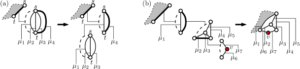
Figure 14: (a) Splitting a P-node into two P-nodes, the vertex $v$ fixed to the outer face is contained in the thick edges. (b) Contracting the path from the root to the node containing $v$ in its skeleton.

To sum up, if $\operatorname{skel}(\tau)$ contains $v$, then we simply have to choose an embedding of $\operatorname{skel}(\tau)$ with $v$ on the outer face. Otherwise, we have to fix the virtual edge containing $v$ to the outer face and additionally have to consider the child of $\tau$ corresponding to this virtual edge. For the child we then have essentially the same situation. Either $v$ is contained in its skeleton, then the embedding is fixed to the unique embedding having $v$ on the outer face or $v$ is contained in some virtual edge. However, then the embedding of the skeleton is again completely fixed (P-nodes have to be split up first) and we can continue with the child corresponding to the virtual edge containing $v$. This yields a path of nodes starting with the root $\tau$ having a completely fixed embedding only depending on the embedding $\mathcal{E}_{\tau}$ chosen for $\operatorname{skel}(\tau)$. As the nodes on the path do not represent any embedding choices, we can simply contract the whole path into a single new root node, merging the skeletons on the path, such that the embedding of the new skeleton of the root is still fixed. This contraction is illustrated in Figure 14(b). More precisely, let $\tau$ be the root and let $\varepsilon$ be the edge containing $v$, corresponding to the child $\mu$. Then we merge $\tau$ and $\mu$ by replacing $\varepsilon$ in $\tau$ by the skeleton of $\mu$ without the parent edge. The children of $\mu$ are of course attached to the new root $\tau^{\prime}$ since $\operatorname{skel}(\tau^{\prime})$ contains the corresponding virtual edges. As mentioned before, the embedding of $\operatorname{skel}(\mu)$ was fixed by the requirement that $v$ is on the outer face, thus the new skeleton $\operatorname{skel}(\tau^{\prime})$ has a unique embedding $\mathcal{E}_{\tau^{\prime}}$ inducing $\mathcal{E}_{\tau}$ on $\operatorname{skel}(\tau)$ and having $v$ or the new virtual edge containing $v$ on the outer face. The procedure of merging the root with the child corresponding to the virtual edge containing $v$ is repeated until $v$ is contained in the skeleton of the root. We call the resulting tree the restricted SPQR-tree with respect to the vertex $v$ and to the embedding $\mathcal{E}_{\tau}$ of the root.

To come back to the problem OptimalFlexDraw, we can easily apply the algorithm presented in Section 6.1 to the restricted SPQR-tree. All nodes apart from the root are still S-, P-, Q- or R-nodes and thus the cost functions with respect to the corresponding pertinent graphs can be computed bottom up. The root $\tau$ may have a more complicated skeleton, however, its embedding is fixed, thus we can apply the flow algorithm as before, yielding an optimal drawing with respect to the chosen root $\tau$ and to the embedding $\mathcal{E}_{\tau}$ of $\operatorname{skel}(\tau)$ with the additional requirement that $v$ lies on the outer face. Since the restricted SPQR-tree can be easily computed in linear time for a chosen root $\tau$ and a fixed embedding $\mathcal{E}$ of $\operatorname{skel}(\tau)$, we can compute a $(\tau,\mathcal{E})$-optimal orthogonal representation with the additional requirement that $v$ lies on the outer face in $T_{\operatorname{flow}}(n)$ time, yielding the following theorem.

Theorem 7.

OptimalFlexDraw with the additional requirement that a specific vertex lies on the outer face can be solved in $\mathcal{O}(n\cdot T_{\operatorname{flow}}(n))$ time for convex biconnected instances.

As motivated before, we can use the BC-tree to solve OptimalFlexDraw for instances that are not necessarily biconnected. We obtain the following theorem.

Theorem 8.

OptimalFlexDraw can be solved in $\mathcal{O}(n^{2}\cdot T_{\operatorname{flow}}(n))$ time for convex instances.

Proof.

Let $G$ be a convex instance with positive flexibility of OptimalFlexDraw and let $\mathcal{B}$ be its BC-tree rooted at some B-node $\beta$. We show how to find an optimal drawing of $G$, optimizing over all embeddings represented by $\mathcal{B}$ with respect to the root $\beta$. Then we can simply choose every B-node in $\mathcal{B}$ to be the root once, solving OptimalFlexDraw. The algorithm consumes $\mathcal{O}(n\cdot T_{\operatorname{flow}}(n))$ time for each root $\beta$ and thus the overall running time is $\mathcal{O}(n^{2}\cdot T_{\operatorname{flow}}(n))$. For the block corresponding to the root $\beta$ we use Theorem 6 to find the optimal orthogonal representation. For all other blocks we use Theorem 7 to find the optimal orthogonal representation with the cutvertex corresponding to the parent in $\mathcal{B}$ on the outer face. It remains to stack these orthogonal representations together without causing additional cost. This can be easily done, if a cutvertex that is forced to lie on the outer face has all free incidences in the outer face and every other cutvertex has all free incidences in a single face. The former can be achieved as we can assume orthogonal representations to be tight. If the latter condition is violated by a cutvertex $v$, then $v$ has two incident edges $e_{1}$ and $e_{2}$ and the rotation of $v$ is 0 in both incident faces. If both edges $e_{1}$ and $e_{2}$ have zero bends, we bend along a cycle around $v$ in the flex graph and thus we can assume without loss of generality that $e_{1}$ has a bend. Moving $v$ along $e_{1}$ to this bend yields an orthogonal representation where $v$ has both free incidences in the same face. Thus given the orthogonal representations for the blocks, we can simply stack them together without causing additional cost. ∎

6.3 Computing the Flow

In the previous sections we used $T_{\operatorname{flow}}(n)$ as placeholder for the time necessary to compute a minimum-cost flow in a flow network of size $n$. Most minimum-cost flow algorithms do not consider the case of multiple sinks and sources. However, this is not a real problem as we can simply add a supersink connected to all sinks and a supersource connected to all sources. Unfortunately, the resulting flow network is no longer planar. Orlin gives a strongly polynomial time minimum-cost flow algorithm with running time $\mathcal{O}(m\log n(m+n\log n))$, where $n$ is the number of vertices and $m$ the number of arcs [13]. Since our flow network is planar (plus supersink and supersource) the number of arcs is linear in the number of nodes. Thus with this flow algorithm we have $T_{\operatorname{flow}}(n)\in\mathcal{O}(n^{2}\log^{2}n)$.

Cornelsen and Karrenbauer give a minimum-cost flow algorithm for planar flow networks with multiple sources and sinks consuming $\mathcal{O}(\sqrt{\chi}\,n\log^{3}n)$ time [3], where $\chi$ is the cost of the resulting flow. Since the cost functions in an instance of OptimalFlexDraw may define exponentially large costs in the size of the input, we cannot use this flow algorithm in general to obtain a polynomial time algorithm. However, in practice it does not really make sense to have exponentially large costs. Moreover, in several interesting special cases an optimal solution has cost linear in the number of vertices. We obtain the following results.

Corollary 3.

A convex instance $G$ of OptimalFlexDraw can be solved in $\mathcal{O}(n^{4}\log^{2}n)$ and $\mathcal{O}(\sqrt{\chi}\,n^{3}\log^{3}n)$ time, where $\chi$ is the cost of an optimal solution. The running time can be improved by a factor of $\mathcal{O}(n)$ for biconnected graphs.

7 Conclusion

We presented an efficient algorithm for the problem OptimalFlexDraw that can be seen as the optimization problem corresponding to FlexDraw. As a first step, we considered biconnected 4-planar graphs with a fixed embedding and showed that they always admit a nice drawing, which implies at most three bends per edge except for a single edge on the outer face with up to four bends.

Our algorithm for optimizing over all planar embeddings requires that the first bend on every edge does not cause any cost as the problem becomes $\mathcal{NP}$-hard otherwise. Apart from that restriction we allow the user to specify an arbitrary convex cost function independently for each edge. This enables the user to control the resulting drawing. For example, our algorithm can be used to minimize the total number of bends, neglecting the first bend of each edge. This special case is the natural optimization problem arising from the decision problem FlexDraw. As another interesting special case, one can require every edge to have at most two bends and minimize the number of edges having more than one bend. This enhances the algorithm by Biedl and Kant [1] generating drawings with at most two bends per edge with the possibility of optimization. Note that in both special cases the cost of an optimal solution is linear in the size of the graph, yielding a running time in $\mathcal{O}(n^{\frac{7}{2}}\log^{3}n)$ ($\mathcal{O}(n^{\frac{5}{2}}\log^{3}n)$ if the graph is biconnected).

References

- [1] T. Biedl and G. Kant. A Better Heuristic for Orthogonal Graph Drawings. Comput. Geom., 9(3):159–180, 1998.
- [2] T. Bläsius, M. Krug, I. Rutter, and D. Wagner. Orthogonal Graph Drawing with Flexibility Constraints. In Graph Drawing (GD’10), volume 6502 of LNCS, pages 92–104. Springer, 2011.
- [3] S. Cornelsen and A. Karrenbauer. Accelerated Bend Minimization. In Graph Drawing (GD’11), volume 7034 of LNCS, pages 111–122. Springer, 2012.
- [4] G. Di Battista, G. Liotta, and F. Vargiu. Spirality and Optimal Orthogonal Drawings. SIAM J. Comput., 27(6):1764–1811, 1998.
- [5] G. Di Battista and R. Tamassia. On-Line Maintenance of Triconnected Components with SPQR-Trees. Algorithmica, 15(4):302–318, 1996.
- [6] G. Di Battista and R. Tamassia. On-Line Planarity Testing. SIAM J. Comput., 25(5):956–997, 1996.
- [7] J. Edmonds and R. M. Karp. Theoretical Improvements in Algorithmic Efficiency for Network Flow Problems. J. ACM, 19:248–264, 1972.
- [8] U. Fößmeier and M. Kaufmann. Drawing High Degree Graphs with Low Bend Numbers. In Graph Drawing (GD’95), LNCS, pages 254–266. Springer, 1995.
- [9] A. Garg and R. Tamassia. On the Computational Complexity of Upward and Rectilinear Planarity Testing. SIAM J. Comput., 31(2):601–625, 2001.
- [10] C. Gutwenger and P. Mutzel. A Linear Time Implementation of SPQR-Trees. In Graph Drawing (GD’00), volume 1984 of LNCS, pages 77–90. Springer, 2001.
- [11] G. W. Klau and P. Mutzel. Quasi-Orthogonal Drawing of Planar Graphs. Technical report, Max-Planck-Institut für Informatik, Saarbrücken, Germany, 1998.
- [12] A. Morgana, C. P. de Mello, and G. Sontacchi. An Algorithm for 1-bend Embeddings of Plane Graphs in the Two-Dimensional Grid. Discr. Appl. Math., 141(1-3):225–241, 2004.
- [13] J. B. Orlin. A Faster Strongly Polynomial Minimum Cost Flow Algorithm. Oper. Res., 41:338–350, 1993.
- [14] I. Rutter. The Many Faces of Planarity – Matching, Augmentation, and Embedding Algorithms for Planar Graphs –. PhD thesis, Fakultät für Informatik, Karlsruher Institut für Technologie (KIT), 2011.
- [15] R. Tamassia. On Embedding a Graph in the Grid with the Minimum Number of Bends. SIAM J. Comput., 16(3):421–444, 1987.
- [16] R. Tamassia, G. Di Battista, and C. Batini. Automatic Graph Drawing and Readability of Diagrams. IEEE Trans. Syst. Man Cybern., 18(1):61–79, 1988.
- [17] S. Tayu, K. Nomura, and S. Ueno. On the Two-Dimensional Orthogonal Drawing of Series-Parallel Graphs. Discr. Appl. Math., 157(8):1885–1895, 2009.
- [18] H. Whitney. Non-Separable and Planar Graphs. Transactions of the American Mathematical Society, 34(2):339–338, April 1932.