Probing Primordial Non-Gaussianity with Weak Lensing Minkowski Functionals

Abstract

We study the cosmological information contained in the Minkowski Functionals (MFs) of weak gravitational lensing convergence maps. We show that the MFs provide strong constraints on the local type primordial non-Gaussianity parameter $f_{{\rm NL}}$. We run a set of cosmological $N$-body simulations and perform ray-tracing simulations of weak lensing, to generate 100 independent convergence maps of 25 deg² field-of-view for $f_{\rm NL}=-100,0$ and $100$. We perform a Fisher analysis to study the degeneracy among other cosmological parameters such as the dark energy equation of state parameter $w$ and the fluctuation amplitude $\sigma_{8}$. We use fully nonlinear covariance matrices evaluated from 1000 ray-tracing simulations. For the upcoming wide-field observations such as Subaru Hyper Suprime-Cam survey with the proposed survey area of 1500 deg², the primordial non-Gaussianity can be constrained with a level of $f_{{\rm NL}}\sim 80$ and $w\sim 0.036$ by weak lensing MFs. If simply scaled by the effective survey area, a 20000 deg² lensing survey using Large Synoptic Survey Telescope will give constraints of $f_{{\rm NL}}\sim 25$ and $w\sim 0.013$. We show that these constraints can be further improved by a tomographic method using source galaxies in multiple redshift bins.

1 INTRODUCTION

An array of recent precise cosmological observations such as the cosmic microwave background (CMB) anisotropies (Komatsu et al., 2011) and the large-scale structure (e.g. Tegmark et al., 2006; Reid et al., 2010b) established the so-called standard cosmological model, in which the energy content of the present-day universe is dominated by dark energy and dark matter. The standard model assumes that the primordial density fluctuations are generated via inflation in the very early universe, which seeded eventually all the rich structures of the universe we see today. The density fluctuations generated through the mechanism generally follow Gaussian statistics. Deviations from primordial Gaussianity would provide interesting information on the early universe. For example, some inflationary models predict generation of non-Gaussian density fluctuations, called the primordial non-Gaussianity (for a review, see Bartolo et al., 2004).

For the so-called local type non-Gaussian models, the initial curvature fluctuation $\Phi$ is expressed by the Taylor expansion of a Gaussian field $\Phi_{\rm G}$

$$\Phi(\mbox{\boldmath$x$})=\Phi_{\rm G}(\mbox{\boldmath$x$})+f_{{\rm NL}}\left(\Phi_{\rm G}^{2}(\mbox{\boldmath$x$})-\langle\Phi_{G}^{2}(\mbox{\boldmath$x$})\rangle\right)+\cdots.$$ (1)

The leading coefficient $f_{\rm NL}$ determines the strength of the non-Gaussianity (Komatsu & Spergel, 2001). The amplitude of $f_{\rm NL}$ depends on the perturbation generation mechanism and hence on the physics of inflation.

There have been several observational probes of $f_{\rm NL}$. For example, the bispectrum of the CMB anisotropies is shown to be a powerful probe of $f_{\rm NL}$ (Komatsu et al., 2011). The abundance and the distribution of galaxies and galaxy clusters can be also used to constrain $f_{\rm NL}$. Primordial non-Gaussianity induces a strong scale-dependence in the power and bi-spectra of biased objects at large length scales and changes the abundance of very massive clusters (e.g. Dalal et al., 2008; Nishimichi et al., 2010; Shandera et al., 2011). It is important to note that the large-scale clustering of galaxies and galaxy cluster can be used to constrain or possibly detect scale-dependent non-Gaussianity which evades the CMB constraints (e.g. Lo Verde et al., 2008). de Bernardis et al. (2010) derived constraints on $f_{\rm NL}$ by combining the CMB anisotropies and galaxy clustering data. However, galaxies are thought to be biased tracers of underlying matter distribution. (e.g. Croton et al., 2007; Reid et al., 2010a). In order to avoid uncertainties associated with complicated galaxy bias, it would be ideal probe the dark matter distribution directly.

Gravitational lensing is a powerful method to study dark matter distribution (e.g. Oguri et al., 2012). Future weak lensing surveys are aimed at measuring cosmic shear over a wide area of more than a thousand square degrees. Such observational programmes include Subaru Hyper Suprime-Cam (HSC) , the Dark Energy Survey (DES) , and the Large Synoptic Survey Telescope (LSST) . Space missions such as Euclid and WFIRST are also promising to conduct a very wide-field cosmology survey. The large set of cosmic shear data will enable us to greatly improve the constraints on cosmological parameters which include primordial non-Gaussianity (e.g. Oguri & Takada, 2011).

There are many statistics proposed to characterize the large-scale matter distribution. Minkowski Functionals (MFs) are among useful statistics to extract the non-Gaussian information from two-dimensional or three-dimensional maps. For example, the full set of CMB MFs has already given comparable constraints to those obtained using the CMB bispectrum (Hikage et al., 2008). Matsubara & Jain (2001) and Sato et al. (2001) studied $\Omega_{m}$-dependence of weak lensing MFs. More recently, Kratochvil et al. (2012) showed that the lensing MFs contain significant cosmological information, beyond the power-spectrum. It is important and timely to study weak lensing MFs using fully nonlinear simulations of cosmic structure formation.

In this paper, we forecast for future weak lensing surveys using MFs. In particular, we examine their ability to constrain the amplitude of the local-type primordial non-Gaussianity. We run a large set of $N$-body simulations and then perform ray-tracing simulations of gravitational lensing. We measure MFs directly from the highly-resolved mock cosmic shear maps. We perform a full Fisher analysis to study the degeneracy among other cosmological parameters, especially the dark energy equation of state $w=P/\rho$. We propose to use future cosmology surveys to constrain, or possibly detect, primordial non-Gaussianities.

The rest of the present paper is organized as follows. In Section 2, we describe the details of $N$-body simulations and our ray-tracing simulations of gravitational lensing. In Section 3, we summarize the basics of MFs. In Section 4, we show the results of a Fisher analysis using MFs. We clarify the degeneracy among the three parameters we consider. Concluding remarks and discussions are given in Section 5.

2 METHODOLOGY

2.1 $N$-body Simulations

We run a number of cosmological $N$-body simulations to generate weak lensing convergence maps. We use the parallel Tree-Particle Mesh code Gadget2 (Springel, 2005). Each simulation is run with $256^{3}$ dark matter particles. We run simulations of two different volumes, $240$ and $480\ h^{-1}$Mpc on a side. We generate the initial conditions following a parallel code developed in Nishimichi et al. (2009) and Valageas & Nishimichi (2011), which employs the second-order Lagrangian perturbation theory (e.g. Crocce et al., 2006). The initial redshift is set to $z_{\rm init}=50$, where we compute the linear matter transfer function using CAMB (Lewis et al., 2000). We then follow Nishimichi et al. (2010) to add non-Gaussian corrections to the initial conditions. For our fiducial cosmology, we adopt the following parameters: matter density $\Omega_{m}=0.2726$, dark energy density $\Omega_{\Lambda}=0.7274$, Hubble parameter $h=0.704$ and the scalar spectral index $n_{s}=0.963$. These parameters are consistent with the WMAP 7-year results (Komatsu et al., 2011). For the primordial non-Gaussianity parameter, we adopt $f_{\rm NL}=0,\pm 100$. To investigate the degeneracy of the cosmological parameters, we also run the same set of simulations for different $w$ and $\sigma_{8}$, where $\sigma_{8}$ is the rms of the density field on 8 $h^{-1}$Mpc. For these runs, we fix the amplitude of curvature fluctuations $\Delta_{\cal R}^{2}=2.441\times 10^{-9}$ at the pivot scale $k=0.002{\rm Mpc}^{-1}$. For $w=-0.8,-1.0,$ and $-1.2$, the resulting $\sigma_{8}$ is equal to 0.753, 0.809, and 0.848, respectively. We summarize the simulation parameters in Table 1.

After performing the simulations with $w=-0.8$ and $w=-1.2$, we found that our code had a bug in converting the physical time to the cosmic expansion parameter in the part where gravitational acceleration due to particle-particle interactions is calculated. This bug affected the results for $w=-0.8$ and $w=-1.2$. However, we have explicitly checked that the effect was very minor and that the statistics we use below were hardly affected. For example, the matter power spectra at $z=0$ after and before the bug was fixed differ less than 0.1 percent in the power amplitude at $0.04<k<1\,h/{\rm Mpc}$.

2.2 Ray Tracing Simulations

For ray-tracing simulations of gravitational lensing, we generate light-cone outputs using multiple simulation boxes in the following manner. The small- and large-volume simulations are placed to cover a past light-cone of a hypothetical observer with angular extent $5^{\circ}\times 5^{\circ}$, from redshift $z=0$ to $z\sim 3.5$, similarly to the methods in White & Hu (2000) and Hamana & Mellier (2001). We follow Sato et al. (2009) in order to simulate gravitational lensing signals. Details of the configuration are found there.

We set the initial ray directions on $2048^{2}$ grids. The corresponding angular grid size is $5^{\circ}/2048\sim 0.15$ arcmin. To avoid the same structure aligned along the line of sight, we shift randomly the $N$-body simulation boxes. In addition, we use simulation outputs from independent realizations when generating the light-cone outputs. We generate 100 independent convergence maps from 20 $N$-body simulations for each cosmological model. We fix the redshift of the source galaxies to $z_{\rm source}=1.0,1.5$.

It is well-known that the intrinsic ellipticities of source galaxies induce noises to lensing shear maps. Assuming intrinsic ellipticities are uncorrelated, we compute the noise to convergence as

$$\langle\kappa_{\rm noise}(x,y)\kappa_{\rm noise}(x^{\prime},y^{\prime})\rangle=\frac{\sigma_{\gamma}^{2}}{n_{\rm gal}A_{\rm pix}}\delta_{xx^{\prime}}\delta_{yy^{\prime}},$$ (2)

where $\delta_{xx^{\prime}}$ is the Kronecker delta symbol, $n_{\rm gal}$ is the number density of source galaxies, $A_{\rm pix}$ is the solid angle of a pixel, and $\sigma_{\gamma}$ is the rms of the shear noise. Throughout this paper, we adopt $\sigma_{\gamma}=0.4$ and assume that the total number density of the source galaxies is 30 galaxies/${\rm arcmin}^{2}$. These are typical values for a weak lensing survey using Subaru telescope (e.g. Miyazaki et al., 2007). When we study a tomographic method (see Section 5), we assume $n_{\rm gal}=15\ {\rm galaxies}/{\rm arcmin}^{2}$ at $z_{\rm source}=1.0$ and $1.5$ . To simulate a more realistic survey, we add the Gaussian noises following Eq.(2) to our simulated maps. Then we perform the Gaussian filtering to the noisy lensing maps. We set the smoothing scale to 1 arcmin. This choice corresponds to the optimal smoothing scale for the detection of massive halos using weak lensing with $z_{\rm source}=1.0$ (Hamana et al., 2004). We discuss the effect of smoothing on the statistical analysis in Section 5.

3 MINKOWSKI FUNCTIONALS

3.1 Basics

Minkowski Functionals are morphological statistics for some smoothed random field above a certain threshold. In general, for a given $D$-dimensional smoothed field, one can calculate $D+1$ MFs $V_{i}$. On $\mathbb{S}^{2}$, one can define 2+1 MFs $V_{0},V_{1}$ and $V_{2}$. $V_{0}$, $V_{1}$ and $V_{2}$ describe the fraction of area above the threshold, the total boundary length of contours, and the integral of the geodesic curvature $K$ along the contours. Mathematically, for a given threshold $\nu$, MFs are defined as

$$V_{0}(\nu) \equiv \frac{1}{4\pi}\int_{Q_{\nu}}\,{\rm d}S,$$ (3)

$$V_{1}(\nu) \equiv \frac{1}{4\pi}\int_{\partial Q_{\nu}}\,\frac{1}{4}{\rm d}\ell,$$ (4)

$$V_{2}(\nu) \equiv \frac{1}{4\pi}\int_{\partial Q_{\nu}}\,\frac{1}{2\pi}K{\rm d}\ell,$$ (5)

where $Q_{\nu}$ and $\partial Q_{\nu}$ represent the excursion set and the boundary of the excursion set for a smoothed field $u(\mbox{\boldmath$\theta$})$. They are given by

$$Q_{\nu}=\{\mbox{\boldmath$\theta$}\,|\,u(\mbox{\boldmath$\theta$})>\nu\},$$ (6)

$$\partial Q_{\nu}=\{\mbox{\boldmath$\theta$}\,|\,u(\mbox{\boldmath$\theta$})=\nu\}.$$ (7)

We follow Lim & Simon (2012) to calculate the MFs from pixelated convergence maps. In this step, we convert a convergence field $\kappa$ into $x=(\kappa-\langle\kappa\rangle)/\sigma_{0}$ where $\sigma_{0}$ is the standard deviation of a noisy convergence field on a $5^{\circ}\times 5^{\circ}$ map. In binning the thresholds, we set $\Delta x=0.1$ from $x=-5$ to $x=5$. We have checked that the binning is sufficient to reproduce the analytic MFs formula (Tomita, 1986) for mock 1000 maps of Gaussian random fields. Figure 1 shows the measured and averaged MFs for our 100 convergence maps for the $\Lambda$CDM model and for $z_{\rm source}=1$. We also plot the analytic formula of MFs for Gaussian statistics to show the non-Gaussian features of the simulated convergence maps.

3.2 Dependence on $f_{\rm NL}$

Let us first discuss how the primordial non-Gaussianity $f_{\rm NL}$ affects the lensing convergence and the MFs. We define the ratio of MFs with respect to the fiducial $f_{\rm NL}=0$ model as follows:

$$R_{i}(f_{\rm NL})=\frac{V_{i}(x\,;\,f_{\rm NL}\neq 0)}{V_{i}(x\,;\,f_{\rm NL}=0)},\,i=0,1,2.$$ (8)

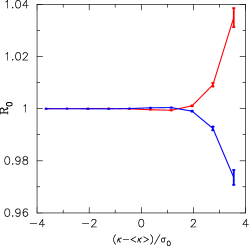
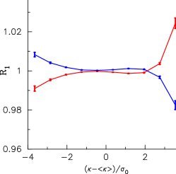
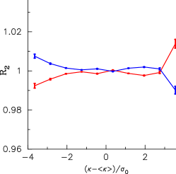
Figure 2: The MFs for our simulated maps with $f_{\rm NL}$. The vertical axis shows the ratio of lensing MFs $V_{i}(f_{\rm NL}=\pm 100)/V_{i}(f_{\rm NL}=0)$. The horizontal axis shows the normalized convergence field $(\kappa-\langle\kappa\rangle)/\sigma_{0}$. The red (blue) points with error bar represent the result from 100 noisy convergence maps with $f_{\rm NL}=+100$ (-100). The source plane locates on $z_{\rm source}=1.0$ and 1 arcmin Gaussian smoothing is adopted.

Figure 2 shows $R_{i}$ from our 100 convergence maps with $z_{\rm source}=1.0$. The effect of $f_{\rm NL}$ appears large in the regime where the normalized convergence $x$ $\stackrel{{\scriptstyle\textstyle>}}{{\textstyle\sim}}$ $3$ for all $V_{i}$s. This simply reflects the fact that $f_{\rm NL}$ affects the number of very massive halos with mass $\sim 10^{15}h^{-1}M_{\odot}$ which yield $x\mbox{\raisebox{-4.30554pt}{$\stackrel{{\scriptstyle\textstyle>}}{{\textstyle\sim}}$ }}3$ (see also Hamana et al., 2004). The abundance of the massive halos at $z=0.5$ is larger by $\sim O(10\%)$ for $f_{\rm NL}=100$ compared to $f_{\rm NL}=0$ (Nishimichi et al., 2010). Then the fraction of area ($V_{0}$) with very high convergence increases for positive $f_{\rm NL}$, and the total length of contours ($V_{1}$) increases too. Interestingly, $f_{\rm NL}$ also affects $V_{1}$ and $V_{2}$ at small $x$. Because the MFs, $V_{0},V_{1},V_{2}$ are not independent statistics, their correlations need to be considered. We use all the MFs combined together in our statistical analysis below, in order to extract the full cosmological information and to derive an accurate constraint on $f_{\rm NL}$.

4 RESULT

4.1 Fisher analysis

We perform a Fisher analysis to make forecasts for parameter constraints on $f_{\rm NL}$, $w$, and $\sigma_{8}$ for future weak lensing surveys.

For a multivariate Gaussian likelihood, the Fisher matrix $F_{ij}$ can be written as

$$F_{ij}=\frac{1}{2}{\rm Tr}\left[A_{i}A_{j}+C^{-1}M_{ij}\right],$$ (9)

where $A_{i}=C^{-1}\partial C/\partial\xi_{i}$, $M_{ij}=2\left(\partial\mu/\partial\xi_{i}\right)\left(\partial\mu/\partial\xi_{j}\right)$, $C$ is the data covariance matrix, $\mu$ is the assumed model, and $\mbox{\boldmath$\xi$}=(f_{\rm NL},\,w,\,\sigma_{8})$. For lensing MFs, $\mu$ corresponds to $V_{0}$, $V_{1}$, and $V_{2}$ for different bins.

We estimate $\mu$ by averaging MFs over our 100 (noisy) convergence maps. To calculate $M_{ij}$, we approximate the first derivative of MFs by the cosmological parameter $\xi_{i}$ as follows

$$\frac{\partial\mu}{\partial\xi_{i}}=\frac{\mu(\xi_{i}+\delta\xi^{(1)}_{i})-\mu(\xi_{i}+\delta\xi^{(2)}_{i})}{\delta\xi^{(1)}_{i}-\delta\xi^{(2)}_{i}}.$$ (10)

We use the data set of the three MFs for $z_{\rm source}=1.0$ or/and $1.5$. We use 10 bins in the range of $x=[-3,3]$. We have checked this binning is sufficient to produce robust results in the following analysis. In this range of $x$, Eq. (10) gives smooth estimate for $M_{ij}$. In total, we need $60\times 60$ MFs covariance matrix for the Fisher analysis. For this purpose, we use 1000 convergence maps made by Sato et al. (2009). These maps have the same design as our convergence maps, but are generated for slightly different cosmological parameters (consistent with WMAP 3-years results (Spergel et al., 2007)). We essentially assume that the dependence of the covariance matrix to cosmological parameters is unimportant.

We also take into account the constraints from the CMB priors expected from the Planck satellite mission. When we compute the Fisher matrix for the CMB, we use the Markov-Chain Monte-Carlo (MCMC) engine for exploring cosmological parameter space COSMOMC (Lewis & Bridle, 2002). We consider the parameter constraints from the angular power spectra of temperature anisotropies, $E$-mode polarization and their cross-correlation. For MCMC, in addition to $\sigma_{8}$ and $w$, our independent variables include the matter density $\Omega_{m}h^{2}$, the baryon density $\Omega_{b}h^{2}$, Hubble parameter $h$, reionization optical depth $\tau$, and the scalar spectral index $n_{s}$. To examine the pure power of lensing MFs to constrain $f_{\rm NL}$, we do not include any constraints on $f_{\rm NL}$ from the CMB. Assuming that the constraints from the CMB and the lensing MFs are independent, we express the total Fisher matrix as

$$\mbox{\boldmath$F$}=\mbox{\boldmath$F$}_{\rm MFs}+\mbox{\boldmath$F$}_{\rm CMB}.$$ (11)

When we include the CMB priors by Eq. (11), we marginalize over the other cosmological parameters except $f_{\rm NL}$, $w$ and $\sigma_{8}$.

Strictly speaking, one needs to consider a multivariate non-Gaussian likelihood because MFs are non-Gaussian estimator. In the present paper, we employ the Fisher analysis that assumes a local Gaussian likelihood in the parameter space. Note however that, because we use fully nonlinear covariance matrices evaluated from 1000 ray-tracing simulations, our analysis appropriately includes non-Gaussian error contributions. Non-Gaussian error will include the contribution of four-point statistics at least (cf. Munshi et al., 2012b). It is illustrative to show the impact of non-Gaussian errors of MFs for parameter estimation. For comparison, we generate Gaussian covariance matrices by using 1000 Gaussian convergence maps. We have found that the resulting constraint on cosmological parameters is degraded by a factor of a few percent compared to the case with Gaussian errors.

4.2 Forecasts

We show the forecast for the upcoming survey such as Subaru Hyper Suprime-Cam (HSC) and the Large Synoptic Survey Telescope (LSST). We consider two surveys with an area coverage of 1500 ${\rm deg}^{2}$ and 20000 ${\rm deg}^{2}$; the former is for HSC, and the latter is for LSST. We first derive constraints on the cosmological parameters for a 25 ${\rm deg}^{2}$ area survey, for which we have the full covariance matrix. Then we simply scale the covariance matrix by a factor of $25/1500=1/60$ or $25/20000=1/800$ for the two surveys considered.

Figure 3 shows the two-dimensional confidence contours for HSC (1500 ${\rm deg}^{2}$), in each case marginalized over other parameters. In each panel, the blue line shows the constraint from lensing MFs only and the red one is for the case of lensing MFs and the Planck priors. The ellipses shown in this figure correspond to the $68\%$ confidence level from the Fisher analysis. Our fiducial model in this analysis is $(f_{\rm NL}\,,w\,,\sigma_{8})=(0\,,-1\,,0.809)$. With the Planck priors, we can constrain $f_{\rm NL}$ with a level of $\sim 80$ by using the source plane at $z_{\rm source}=1.0$, after marginalized over $w$ and $\sigma_{8}$.

For the upcoming multiple-band imaging surveys such as HSC and LSST, it is possible to obtain photometric redshifts for the source galaxies. It is interesting to study how the parameter constraints can be improved by using source galaxies at higher redshifts. To this end, we perform the same analysis assuming the source galaxies are located at two redshifts, $z_{\rm source}=1.0$ and 1.5. We show the Fisher analysis result in the right panel of Figure 3. We see the constraint on $f_{\rm NL}$ is improved by a factor of $\sim$ 1.5 with the two redshift bins. We summarize the marginalized constraints on $f_{\rm NL}$ in Table 2.

5 CONCLUSION AND DISCUSSION

We have studied the ability of weak lensing MFs to constrain the local type primordial non-Gaussianity. We have performed 20 $N$-body simulations and 100 independent ray-tracing simulations for each of the seven cosmological models that differ in $f_{\rm NL}$, $w$ and $\sigma_{8}$. We have then performed a Fisher analysis using the large set of mock lensing maps, to obtain confidence limits for cosmological parameters.

The MFs are sensitive probes of $f_{\rm NL}$, especially at high convergence values, because such high convergence regions are associated with massive halos with $\stackrel{{\scriptstyle\textstyle>}}{{\textstyle\sim}}$ $10^{15}h^{-1}M_{\odot}$, of which the abundance is sensitive to $f_{\rm NL}$. We also find that the three MFs, $V_{0},V_{1}$ and $V_{2}$, are affected differently by $f_{\rm NL}$. This means that combining the three MFs gives tighter constraints on $f_{\rm NL}$.

From a Fisher analysis, we have obtained the following results. For source galaxies at $z_{\rm source}=1.0$, the primordial non-Gaussianity is constrained with a level of $f_{\rm NL}\sim 80$ for HSC survey with a 1500 ${\rm deg}^{2}$ survey area. The constraints can be improved by selecting source galaxies in multiple redshift bins. We find that the constraint on $f_{\rm NL}$ is improved to $\sim 50$, i.e., by a factor of $\sim$ 1.5 if we use source galaxies at $z_{\rm source}=1.0$ and $1.5$. This is largely because the degeneracy between $\sigma_{8}$ and $w$ is broken due to information contained in the matter distribution at different redshifts. We have also tested how the number density of the source galaxies affects our analysis. We have re-analyzed the case of $n_{\rm gal}=30$ galaxies$/{\rm arcmin}^{2}$ for a fixed source plane at $z_{\rm source}=1.0$. The constraint on $f_{\rm NL}$ is improved only by a factor of $\sim$ 5 % in this case. We argue that the “tomographic” information using the multiple source planes is useful to derive accurate constraints on $f_{\rm NL}$, even though one then needs to use a smaller number of source galaxies at each of the source planes.

Ultimately, for a LSST-like survey with a 20000 ${\rm deg}^{2}$ area, we can obtain the constraint of $f_{\rm NL}\sim 25$ with $z_{\rm source}=1.0$, and $f_{\rm NL}\sim 15$ with $z_{\rm source}=1.0$ and $1.5$. In principle, these constraints will be further improved by including the high sigma bins of MFs because the higher convergence region is more sensitive to $f_{\rm NL}$. We will continue our study along this line using a larger set of simulations of larger volumes.

Finally, we discuss possible technical improvements in using the MFs of weak lensing maps. First, we have checked how the smoothing scale on the convergence maps affects our analysis. We have performed a Fisher analysis using the maps with smoothing of 0.5 arcmin, 1 arcmin, 2 arcmin and 5 arcmin. Smoothing with $\sim 1$ arcmin has turned out to be optimal for the targeted future surveys, yielding the best constraints. This is explained qualitatively by the fact that only the large-scale, linear structure is probed with large smoothing scales, whereas for smaller smoothing scales, the intrinsic shape noise becomes large. We note that the angular-scale dependence of MFs itself can provide more information. For example, the angular-scale dependence can be used to separate primordial non-Gaussianities from gravity-induced non-Gaussianities (e.g. Munshi et al., 2012a, b; Kratochvil et al., 2012). One could further improve the cosmological constraints by combining MFs with various smoothing scales and their evolutions. Evaluating MFs is complicated when an observed map include masked regions. Also, instrumental and atmospheric systematics can easily compromise the measurement of lensing MFs. These issues certainly warrants further extensive studies. The upcoming wide-field surveys will provide highly-resolved lensing maps. Our study in the present paper may be useful to properly analyze the data and extract cosmological information from them.

Figure 1: The Minkowski Functionals from our simulated convergence maps. The solid lines show the average MFs over 100 maps with the fiducial cosmological parameters. The dashed lines show the analytic formula of MFs for the Gaussian field (Tomita, 1986). We use 100 convergence maps located on $z_{\rm source}=1$.

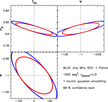
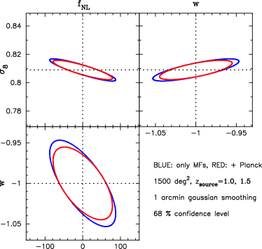
Figure 3: We plot 1-$\sigma$ confidence level by weak lensing MFs for Subaru HSC survey (1500 ${\rm deg}^{2}$). The left panel shows the constraints on $f_{\rm NL}$, $w$ and $\sigma_{8}$ for the case with $z_{\rm source}=1.0$. The right panel shows the constraints obtained by a tomographic survey with $z_{\rm source}=1.0$ and $1.5$. The blue line shows the constraints from lensing MFs only and the red one represents those by MFs and the Planck priors.

	$f_{\rm NL}$	$w_{\rm DE}$	$\sigma_{8}$	# of $N$-body sims	# of maps
fiducial	0	-1.0	0.809	20	100
high $w_{\rm DE}$	0	-0.8	0.753	20	100
low $w_{\rm DE}$	0	-1.2	0.848	20	100
high $f_{\rm NL}$	100	-1.0	0.809	20	100
low $f_{\rm NL}$	-100	-1.0	0.809	20	100
high $\sigma_{8}$	0	-1.0	0.848	20	100
low $\sigma_{8}$	0	-1.0	0.753	20	100

Table 1: Parameters for our $N$-body simulations. For each model, we run 20 $N$-body realizations and generate 100 weak lensing convergence maps.

	$z_{\rm source}=1.0$	$z_{\rm source}=1.0,\,1.5$
MFs only (1500 ${\rm deg}^{2}$)	96.8	57.9
MFs + Planck (1500 ${\rm deg}^{2}$)	78.5	52.1
MFs only (20000 ${\rm deg}^{2}$)	26.5	15.8
MFs + Planck (20000 ${\rm deg}^{2}$)	25.8	15.7

Table 2: The 1-$\sigma$ constraint on $f_{\rm NL}$ when marginalized over $w$ and $\sigma_{8}$. We consider two surveys with a survey area of 1500 ${\rm deg}^{2}$ (HSC) and 20000 ${\rm deg}^{2}$ (LSST). The analysis includes the intrinsic noise from source galaxies with the number density of $n_{\rm gal}=15\ {\rm galaxies}/{\rm arcmin}^{2}$ at each source redshift.

References

- Bartolo et al. (2004) Bartolo, N., Komatsu, E., Matarrese, S., & Riotto, A. 2004, Phys. Rep., 402, 103
- Crocce et al. (2006) Crocce, M., Pueblas, S., & Scoccimarro, R. 2006, MNRAS, 373, 369
- Croton et al. (2007) Croton, D. J., Gao, L., & White, S. D. M. 2007, MNRAS, 374, 1303
- Dalal et al. (2008) Dalal, N., Doré, O., Huterer, D., & Shirokov, A. 2008, Phys. Rev. D, 77, 123514
- de Bernardis et al. (2010) de Bernardis, F., Serra, P., Cooray, A., & Melchiorri, A. 2010, Phys. Rev. D, 82, 083511
- Eifler et al. (2009) Eifler, T., Schneider, P., & Hartlap, J. 2009, A&A, 502, 721
- Hamana & Mellier (2001) Hamana, T., & Mellier, Y. 2001, MNRAS, 327, 169
- Hamana et al. (2004) Hamana, T., Takada, M., & Yoshida, N. 2004, MNRAS, 350, 893
- Hikage et al. (2008) Hikage, C., Matsubara, T., Coles, P., et al. 2008, MNRAS, 389, 1439
- Komatsu & Spergel (2001) Komatsu, E., & Spergel, D. N. 2001, Phys. Rev. D, 63, 063002
- Komatsu et al. (2011) Komatsu, E., Smith, K. M., Dunkley, J., et al. 2011, ApJS, 192, 18
- Kratochvil et al. (2012) Kratochvil, J. M., Lim, E. A., Wang, S., et al. 2012, Phys. Rev. D, 85, 103513
- Lewis & Bridle (2002) Lewis, A., & Bridle, S. 2002, Phys. Rev., D66, 103511
- Lewis et al. (2000) Lewis, A., Challinor, A., & Lasenby, A. 2000, Astrophys. J., 538, 473
- Lim & Simon (2012) Lim, E. A., & Simon, D. 2012, J. Cosmology Astropart. Phys, 1, 48
- Lo Verde et al. (2008) Lo Verde, M., Miller, A., Shandera, S., & Verde, L. 2008, J. Cosmology Astropart. Phys, 4, 14
- Matsubara & Jain (2001) Matsubara, T., & Jain, B. 2001, ApJ, 552, L89
- Miyazaki et al. (2007) Miyazaki, S., Hamana, T., Ellis, R. S., et al. 2007, ApJ, 669, 714
- Munshi et al. (2012a) Munshi, D., Smidt, J., Joudaki, S., & Coles, P. 2012a, MNRAS, 419, 138
- Munshi et al. (2012b) Munshi, D., van Waerbeke, L., Smidt, J., & Coles, P. 2012b, MNRAS, 419, 536
- Nishimichi et al. (2010) Nishimichi, T., Taruya, A., Koyama, K., & Sabiu, C. 2010, J. Cosmology Astropart. Phys, 7, 2
- Nishimichi et al. (2009) Nishimichi, T., Shirata, A., Taruya, A., et al. 2009, PASJ, 61, 321
- Oguri et al. (2012) Oguri, M., Bayliss, M. B., Dahle, H., et al. 2012, MNRAS, 420, 3213
- Oguri & Takada (2011) Oguri, M., & Takada, M. 2011, Phys. Rev. D, 83, 023008
- Reid et al. (2010a) Reid, B. A., Verde, L., Dolag, K., Matarrese, S., & Moscardini, L. 2010a, J. Cosmology Astropart. Phys, 7, 13
- Reid et al. (2010b) Reid, B. A., Percival, W. J., Eisenstein, D. J., et al. 2010b, MNRAS, 404, 60
- Sato et al. (2001) Sato, J., Takada, M., Jing, Y. P., & Futamase, T. 2001, ApJ, 551, L5
- Sato et al. (2009) Sato, M., Hamana, T., Takahashi, R., et al. 2009, ApJ, 701, 945
- Shandera et al. (2011) Shandera, S., Dalal, N., & Huterer, D. 2011, J. Cosmology Astropart. Phys, 3, 17
- Spergel et al. (2007) Spergel, D. N., Bean, R., Doré, O., et al. 2007, ApJS, 170, 377
- Springel (2005) Springel, V. 2005, MNRAS, 364, 1105
- Tegmark et al. (2006) Tegmark, M., Eisenstein, D. J., Strauss, M. A., et al. 2006, Phys. Rev. D, 74, 123507
- Tomita (1986) Tomita, H. 1986, Progress of Theoretical Physics, 76, 952
- Valageas & Nishimichi (2011) Valageas, P., & Nishimichi, T. 2011, A&A, 527, A87
- White & Hu (2000) White, M., & Hu, W. 2000, ApJ, 537, 1