A Transfer Matrix Approach to Electron Transport in Graphene through Arbitrary Electric and Magnetic Potential Barriers

Abstract

A transfer matrix method is presented for solving the scattering problem for the quasi one-dimensional massless Dirac equation applied to graphene in the presence of an arbitrary inhomogeneous electric and perpendicular magnetic field. It is shown that parabolic cylindrical functions, which have previously been used in literature, become inaccurate at high incident energies and low magnetic fields. A series expansion technique is presented to circumvent this problem. An alternate method using asymptotic expressions is also discussed and the relative merits of the two methods are compared.

Keywords: graphene,transfer matrix method, Frobenius method, parabolic cylindrical functions, wave equation

1 Introduction

Graphene’s [1, 2] near perfect two-dimensional configuration and its unique electronic properties[3, 4] have made it one of the widely studied materials in recent times. Its electrons have been found to obey a linear dispersion relation near the Fermi energy which makes them behave like massless relativistic particles in two dimensions. As a result, they obey the massless Dirac equation instead of the Schödinger equation. One of the important consequences of the relativistic behaviour of transport electrons is their inability to be confined by an electrostatic barrier, a phenomenon known as Klein tunnelling [5]. The alternate strategy of confining these Dirac fermions using magnetic fields has been proposed[6, 7]. Consequently, there has been a lot of interest in electron transport through magnetic barriers in graphene. Moreover, building functional electronic devices using graphene relies on being able to control the electronic transport by the application of electromagnetic fields. In this context, electron transmission through varying regularly and irregularly shaped barriers of both scalar and vector potentials becomes an important problem. Proper analysis of such barriers calls for the development of efficient numerical techniques.

In this work, we are interested in developing a general algorithm for the calculation of electron transmission in graphene through inhomogeneous electric and magnetic fields. We only consider magnetic fields perpendicular to the plane of the graphene sheet. We also restrict ourselves to the quasi one-dimensional problem which implies that the fields are invariant in the y-direction and the electronic plane wave is incident on it at an arbitrary angle.

From a mathematical viewpoint, this involves solving the massless Dirac equation which consists of two first-order coupled ordinary differential equations with arbitrary values of electric and magnetic fields. We use the well-known transfer matrix method to solve this problem. This method has previously been applied to problems in optics [8] and quantum mechanics [9]. It is computationally easy to implement, involving only the multiplication of $2\times 2$ matrices. It has been used to study the scattering problem for the Schrödinger equation.[10, 11]. The method has also been extended to solving any homogeneous ordinary linear differential equation[12].

Transfer matrix methods to solve the electron transport problem in graphene have been studied extensively: [5, 6] have applied it to single magnetic barriers; it has been used in [13] to study the transmission through multiple magnetic barriers in graphene; in [14], it is used for electrostatic barriers in bilayer graphene; in [15, 16] for graphene superlattices; in [17] for fractally arranged magnetic barriers; and in [18] for tunnelling through electric barriers in the presence of a magnetic field.

Although we proceed along similar lines, we show that the parabolic cylindrical functions (Weber functions) that have been used in literature can cause significant numerical difficulties at low magnetic fields or at high incident energies and we use a series expansion to solve the differential equation in order to avoid this problem. This forms the main result of this paper. Thus, we provide a uniform framework though this series expansion method and widen the applicability of the transfer matrix method for a large range of incident energies and magnetic fields. Since the ballistic transport regime of Graphene based device is now being studied extensively both experimentally and theoretically [19], our scheme will be quite useful to understand some of such future experiments. We also discuss an alternative method based on approximating Weber functions by their asymptotic form. This method is applicable only within the asymptotic regime whereas the series method is applicable to the entire range of magnetic fields and energies. We show that our method provides accurate results in this range also.

In the special case when the average length across which the vector potential varies is smaller that the typical magnetic length $l_{B}=\sqrt{({\hbar c})/({eB})}$, the magnetic barrier can be approximated by a delta function. Analytic solutions for magnetic barriers modelled as a series of delta functions are well known[20], [21]. The transfer matrix method is more general and can be used even when this condition doesn’t hold.

Solving the Schrödinger or the Dirac equation includes two different kinds of problems: the eigenvalue problem and the scattering problem. The eigenvalue problem involves finding the energy eigenvalues of the Hamiltonian and is used to find the allowed energy levels of bound states. The scattering problem, which is the one we tackle in this paper, involves the calculation of the transmission and reflection coefficients, formally defined as the ratio of the flux of particles transmitted or reflected from a potential configuration to the flux that is incident on it. It leads to a second order homogeneous differential equation, the ubiquitous wave equation, which in one dimension is given by:

$$\psi^{\prime\prime}(x)+k^{2}(x)\psi(x)=0\quad(k\in\bf{C})$$ (1)

The transfer matrix method involves division of the one-dimensional domain into slices and taking an appropriate approximation of $k^{2}(x)$ in each slice. The equation for each slice is then solved and the continuity conditions are used at the interfaces of two such slices. The exact solution of the equation in each slice depends on the form of $k^{2}(x)$ chosen. For example, for the Schrödinger equation, a piecewise constant approximation of $k^{2}(x)$ leads to complex exponential solutions in each slice and a piecewise linear approximation leads to a solution basis consisting of the Airy functions[22].

In the case of graphene, we consider both scalar potentials (electrostatic fields) and vector potentials (magnetic fields), which lead to a piecewise linear vector potential and a piecewise constant scalar potential. The form of the resulting equation is:

$$\psi(x)^{\prime\prime}+\left[\alpha^{2}-p-(\beta+px)^{2}\right]\psi(x)=0$$ (2)

where $\alpha,\beta,p\in\bf{R}$ and are explained later in detail. This equation admits parabolic cylindrical functions as the solution basis. We show that using these becomes computationally infeasible as $p\rightarrow 0$ which corresponds to low magnetic fields and therefore an alternate solution basis is called for. We obtain this using the Frobenius method and find basis functions that tend to complex exponentials as $p\rightarrow 0$.

It is also necessary to restrict the transfer matrix method to cases where the magnetic field is non-zero only over some closed bounded (compact) interval. This divides space into three regions and the solution in the first and last regions are complex exponentials representing incoming and outgoing waves. From a physical point of view, this condition is necessary because if $\forall x,B\neq 0$, such as with a uniform magnetic field, the wavefunction gets localized along the spatial direction $x$.

In Section 2 are outlined the equations to be solved and the notation used. In Section 3, the transfer matrix method is discussed. In Section 4, methods are outlined to solve Equation 2: Section 4.1 details the method previously found in literature along with its limitations. Section 4.2 is a method based on asymptotic expansions, and Section 4.3 is the proposed alternative series method. Finally, in Section 5, we apply this method to a number of cases and present the results obtained.

Figure 1: Piecewise constant scalar potential and piecewise linear vector potential showing the notation for x coordinates and slices used in the paper

2 Governing Equations

The governing massless Dirac equation is given by $H\psi=E\psi$ where the Hamiltonian is given by

$$H=v_{f}\ \vec{\sigma}.(\vec{p}+e\vec{A}(x))+V(x)$$ (3)

and $\psi=[\psi_{1},\psi_{2}]^{T}$ is the two component wavefunction, $\vec{\sigma}=\sigma_{x}\hat{i}+\sigma_{y}\hat{j}$ with $\sigma_{x,y}$ denoting the Pauli spin matrices.

Both the magnetic field $B$ and scalar potentials $V$ are discretized and the magnetic field $B$ is converted to vector potential $A$ in the Landau gauge. The discretisation scheme that we have used is shown in Figure 1. Slices are numbered from $0$ to $N+1$, with the leftmost and rightmost slices unbounded. The boundaries between slices are denoted by $x_{i}$ with $1\leq i\leq N$. Therefore the i^th slice is bounded by $x=x_{i-1}$ and $x=x_{i}$. We denote the magnetic field, scalar potential, and y component of the vector potential in slice $i$ by the notation $B_{i}$, $V_{i}$, $A_{i}$ respectively.

For well defined transmission and reflection coefficients, it is necessary to have zero magnetic field in the first and last slice, $B_{0}=B_{N+1}=0$, so that the solution can be expressed as complex exponentials which represent incoming and outgoing plane waves. The only non-zero component of $\vec{A}$ is $A_{y}(x)$ and is denoted by $A$. The functional form of the vector potential in the i^th slice is $A_{i}=C_{i}+B_{i}(x-x_{i-1})$ where $x_{i-1}$ represents the left edge of the i^th slice, with $x_{-1}$ any conveniently chosen value (because $B_{0}=0$), and $C_{i}=\sum_{j=0}^{i-1}B_{j}(x_{j}-x_{j-1})$, $C_{0}=0$.

The equations given above are converted to dimensionless form by defining two new variables. We substitute $x^{\prime}=x/x_{s}$ and $A^{\prime}=A/A_{s}$. These can be also be thought of as scaling factors and as we shall see later, their exact values are important in computations. In terms of these scaled units, $A^{\prime}_{i}=c_{i}+b_{i}(x^{\prime}-\delta_{i-1})$. It can immediately be seen that $b_{i}=B_{i}x_{s}/A_{s}$, $c_{i}=C_{i}/A_{s}$ and $\delta_{i-1}=x_{i-1}/x_{s}$. In terms of individual components and scaled units, Equation 3 is:

$$\frac{-i}{x_{s}}\frac{\partial\psi_{2}}{\partial x^{\prime}}-ik_{y}\psi_{2}+i\frac{e}{\hbar}(-A_{s}A^{\prime}\psi_{2})=(\epsilon-\tilde{v})\psi_{1}$$

$$\frac{-i}{x_{s}}\frac{\partial\psi_{1}}{\partial x^{\prime}}+ik_{y}\psi_{1}+i\frac{e}{\hbar}(A_{s}A^{\prime}\psi_{1})=(\epsilon-\tilde{v})\psi_{2}$$

where $\epsilon=E/\hbar v_{f}$ and $\tilde{v}=V/\hbar v_{f}$ (these have the units of $[L]^{-1}$). The y-invariance of the problem leads to $\frac{\partial}{\partial y}=ik_{y}$ where $k_{y}=\epsilon\sin(\phi)$ with $\phi$ being the angle of incidence. We seek the transmission as a function of $\phi$. The equations are decoupled bearing in mind that $\tilde{v}$ is constant in each slice and $A_{i}^{\prime}=c_{i}+b_{i}(x-\delta_{i-1})$ is a function of $x$. $\psi_{1}$ and $\psi_{2}$ are then governed by the following relations:

$$\frac{\partial^{2}\psi_{1}}{\partial x^{\prime 2}}+\left[x_{s}^{2}(\epsilon-\tilde{v})^{2}-\frac{e}{\hbar}x_{s}A_{s}\frac{\partial A^{\prime}}{\partial x^{\prime}}-x_{s}^{2}\left(k_{y}+\frac{e}{\hbar}A_{s}A^{\prime}\right)^{2}\right]\psi_{1}=0$$ (4)

$$\psi_{2}=\frac{1}{(\epsilon-\tilde{v})}\left[\frac{-i}{x_{s}}\frac{\partial\psi_{1}}{\partial x^{\prime}}+ik_{y}\psi_{1}+i\frac{e}{\hbar}(A_{s}A^{\prime}\psi_{1})\right]$$ (5)

We use the standard technique of calculating $\psi_{1}$ from Equation 4 and calculating $\psi_{2}$ by backsubstituting $\psi_{1}$ in Equation 5. In Section 4, these equations are solved for a particular slice and in Section 3, these solutions are used to construct the transfer matrix and completely solve the transmission problem.

3 The transfer matrix method

The transfer matrix method relies on the availability of two linearly independent analytic solutions of Equation 4 and Equation 5. If the two linearly independent solutions of $\psi_{1}$ are denoted by $\psi_{1}^{A}$ and $\psi_{1}^{B}$, and the corresponding solutions for $\psi_{2}$ are $\psi_{2}^{A}$ and $\psi_{2}^{B}$, the transfer matrix denoted by $M_{i}$ is such that the solution of the i^th slice is given by:

$$\left[\begin{array}[]{c}\psi_{1}\\ \psi_{2}\\ \end{array}\right]=M_{i}\left[\begin{array}[]{c}A_{i}\\ B_{i}\\ \end{array}\right],M(x)=\left[\begin{array}[]{cc}\psi_{1}^{A}(x)&\psi_{1}^{B}(x)\\ \psi_{2}^{A}(x)&\psi_{2}^{B}(x)\end{array}\right]$$ (6)

From the continuity of $\psi_{1}$ and $\psi_{2}$ across the boundaries, we have

$$M_{i}(x_{i})\left[\begin{array}[]{c}A_{i}\\ B_{i}\\ \end{array}\right]=M_{i+1}(x_{i})\left[\begin{array}[]{c}A_{i+1}\\ B_{i+1}\\ \end{array}\right]\quad\forall\quad 0\leq i\leq N$$ (7)

This allows us to formulate a recurrence relation between the coefficients $A_{i},B_{i}$ and $A_{i+1},B_{i+1}$. Continuing in a similar manner, we relate $A_{0},B_{0}$ with $A_{N+1},B_{N+1}$ which then gives us the reflection and transmission coefficients.

$$\left[\begin{array}[]{c}A_{0}\\ B_{0}\\ \end{array}\right]=P\left[\begin{array}[]{c}A_{N+1}\\ B_{N+1}\\ \end{array}\right],P=\prod_{j=0}^{N}M_{j}(x_{j})^{-1}M_{j+1}(x_{j})$$ (8)

We refer to the expression $M_{j}(x_{j-1})M_{j}^{-1}(x_{j})$ occurring in the expression for $P$ as the transfer matrix for the j^th slice. It can be easily proven that this term is independent of the basis functions chosen in that slice.

The expression for the transfer matrix given in Equation 8 can usually be simplified if the solution in each slice can be solved in a local coordinate system with its origin on the left edge of that slice. This can always be done by shifting the origin in the wave equation, Equation 1. Then the matrix $M(x)$ depends only on $x-x_{i-1}$. Thus, if $M(x)=N(x-x_{i-1})$, substitution in Equation 8 gives this formula:

$$P=\prod_{j=0}^{N}N_{j}(x_{j}-x_{j-1})^{-1}N_{j+1}(0)$$ (9)

where $x_{-1}$ is a suitably chosen constant as explained earlier. We have used this expression in our computations.

3.1 Form of incident, transmitted and reflected waves

In the first and last region, the magnetic field is chosen to be zero so that the solution reduces to complex exponentials of the form $\exp(\pm ikx)$ that represent the incident, reflected and transmitted waves.

In contrast to the Schrödinger equation in which $\exp(+ikx)$ represents right propagating waves, and $\exp(-ikx)$ represents left propating waves, in the case of the Dirac equation $\psi_{1}=\exp(+ikx)$ may represent either right or left propagating waves. If, in a slice, $E>V$, the probability flux corresponding to $\psi_{1}=\exp(+ikx)$ is positive implying that the wave is right propagating. On the other hand, if $E<V$, the flux corrresponding to the same wavefunction is negative and so it represents a left propagating wave.

The incident wave, reflected wave and transmitted wave are given by $\exp({s_{0}ik_{0}x})$, $r\exp({-s_{0}ik_{0}x})$ and $t\exp({s_{N+1}ik_{N+1}x})$ respectively where $s_{i}=\textrm{sign}(E-V_{i})$ and $k_{j}=x_{s}\sqrt{(\epsilon-\tilde{v_{j}})^{2}-(k_{y}+\frac{e}{\hbar}A_{s}c_{j})^{2}}$. The corresponding probability currents in the x-direction, within a constant, given by $\psi^{\dagger}\sigma_{x}\psi$ are $J_{i}=2k_{0}/|\epsilon-\tilde{v}_{0}|$, $J_{r}=-2k_{0}|r|^{2}/|\epsilon-\tilde{v}_{0}|$ and $J_{t}=2k_{N+1}|t|^{2}/|\epsilon-\tilde{v}_{N+1}|$. The transmission and reflection coefficients are given by:

$$R =-J_{r}/J_{i}=|r|^{2}$$

$$T =J_{t}/J_{i}=|t|^{2}\frac{k_{N+1}/|\epsilon-\tilde{v}_{N+1}|}{k_{0}/|\epsilon-\tilde{v}_{0}|}$$

If, however $k_{N+1}$ is imaginary, $J_{t}=0$ and hence $T=0$.

The elements of the transfer matrix $P$ (Equation 9) relates the coefficients of the complex exponentials with a positive or negative sign in the first layer to those in the last layer (denoted by $e_{first}\pm$ and $e_{last}\pm$):

$$\left[\begin{array}[]{c}e_{first}+\\ e_{first}-\end{array}\right]=P\left[\begin{array}[]{c}e_{last}+\\ e_{last}-\end{array}\right] ,\quad P=\left[\begin{array}[]{cc}a&b\\ c&d\end{array}\right]$$

The values of $r$ and $t$ to be used in Equation 3.1 depend on the form that the incident, reflected and transmitted waves have; i.e., whether they are represented by complex exponentials with positive or negative signs. The results are summarised in the following table:

$$\begin{array}[]{llcll}E>V_{0},&E>V_{N+1}&:&t=1/a&r=c/a\\ E>V_{0},&E<V_{N+1}&:&t=1/b&r=d/b\\ E<V_{0},&E>V_{N+1}&:&t=1/c&r=a/c\\ E<V_{0},&E<V_{N+1}&:&t=1/d&r=b/d\\ \end{array}$$ (11)

4 Solving the Governing Equations

We now solve equations 4 and 5 and find solution bases $\psi_{1}^{A,B},\psi_{2}^{A,B}$ to construct the transfer matrix used in Equation 9. To this end, we introduce another change of variable with $x^{\prime\prime}=x^{\prime}-\delta$ representing a translation of the origin to the left boundary of each slice. For notational convenience, subscripts indicating the slice number are omitted in this section. Defining dimensionless constants $\alpha=x_{s}(\epsilon-\tilde{v})$, $p=\frac{e}{\hbar}x_{s}A_{s}b$ and $\beta=x_{s}(k_{y}+\frac{e}{\hbar}A_{s}c)$, equations 4 and 5 can be written in the dimensionless form

$$\frac{d^{2}\psi_{1}}{dx^{\prime\prime 2}}+\left[\alpha^{2}-p-(\beta+px^{\prime\prime})^{2}\right]\psi_{1}=0$$ (12)

$$\psi_{2}=\frac{i}{\alpha}\left[\frac{\partial\psi_{1}}{\partial x^{\prime\prime}}+\psi_{1}(\beta+px^{\prime\prime})\right]$$ (13)

4.1 Parabolic Cylindrical function solution

We first discuss the well-known technique of using parabolic cylindrical functions [17],[6],[23] to solve Equation 12 and 13. The parabolic cylindrical equation in standard form is

$$\frac{\partial^{2}\psi}{\partial x^{2}}-\psi\left[\frac{x^{2}}{4}+a\right]=0$$ (14)

Following the notation used by [24], the two linearly independent solutions to the equation are given by $U(a,x)=D_{\nu}(x)$ and $V(a,x)=V_{\nu}(x)$ with $\nu=-(1/2+a)$. Alternatively, $D_{\nu}(x)$ and $D_{\nu}(-x)$ can also be used as linearly independent solutions.

For solving Equation 12, three cases of $p>0$, $p<0$ and $p=0$ (corresponding to positive, negative and zero magnetic field) need to be dealt with separately. When $p=0$, the solutions are complex exponentials:

$$\psi_{1}=e^{\pm i\sqrt{\alpha^{2}-\beta^{2}}x^{\prime\prime}}\\ \psi_{2}=\frac{1}{\alpha}\left[\pm\sqrt{\alpha^{2}-\beta^{2}}+i\beta\right]e^{\pm i\sqrt{\alpha^{2}-\beta^{2}}x^{\prime\prime}}$$ (15)

When $p\neq 0$, the equation can be converted to standard form by substituting $z=\sqrt{{2}/{|p|}}(\beta+px^{\prime\prime})$. The solutions are $\psi_{1}=D_{\nu}(z),V_{\nu}(z),D_{\nu}(-z)$, where either $D_{\nu}(z)$, $V_{\nu}(z)$ or $D_{\nu}(z)$, $D_{\nu}(-z)$ can be used; $\nu$ is given by:

$$\nu=\left\{\begin{array}[]{ll}\frac{\alpha^{2}}{2p}-1&p>0\\ \frac{\alpha^{2}}{2|p|}&p<0\end{array}\right.$$ (16)

The corresponding expression for $\psi_{2}$ given by Equation 13 is:

$$\psi_{2}=\frac{i}{\alpha}\left[-\sqrt{2|p|}{sign}(p)\frac{\partial\psi_{1}}{\partial z}+\psi_{1}z\sqrt{\frac{|p|}{2}}\right]$$ (17)

This can be further simplified by using standard recurrence relations relating $D_{\nu}(z)$ and $V_{\nu}(z)$ to their derivatives and the simplified expressions are:

$$\begin{array}[]{rll}&\quad\psi_{1}=&\quad\psi_{2}=\\ \\ p>0:&D_{\nu}(z)&\frac{i}{\alpha}\sqrt{2p}D_{\nu+1}(z)\\ &D_{\nu}(-z)&\frac{-i}{\alpha}\sqrt{2p}D_{\nu+1}(-z)\\ &V_{\nu}(z)&\frac{i}{\alpha}\sqrt{2p}(\nu+1)V_{\nu+1}(z)\\ \\ p<0:&D_{\nu}(z)&\frac{i}{\alpha}\sqrt{2|p|}(\nu)D_{\nu-1}(z)\\ &D_{\nu}(-z)&\frac{-i}{\alpha}\sqrt{2|p|}(\nu)D_{\nu-1}(-z)\\ &V_{\nu}(z)&\frac{i}{\alpha}\sqrt{2|p|}V_{\nu-1}(z)\end{array}$$ (18)

We now discuss the limitations of this method. The function $D_{\nu}(z)$ has a power-law dependence with $\nu$ and increases at a near-exponential rate with an increase in $\nu$ and reaches $10^{308}$ at around $\nu=300$ which is the maximum representable double precision value on a computer. It can be seen from Equation 16 that the parameter $\nu$ contains the term:

$$\frac{\alpha^{2}}{2|p|}=\frac{x_{s}(\epsilon-\tilde{v})^{2}}{2\frac{e}{\hbar}A_{s}b}=\frac{(\epsilon-\tilde{v})^{2}}{2\frac{e}{\hbar}B}$$ (19)

where the relation $b=B\frac{x_{s}}{A_{s}}$ has been used. From this, it can immediately be seen that $\nu$ increases with an increase in the incident energy $\epsilon$ and increases with a decrease in the magnetic field $B$. Furthermore, the expression for $\nu$ is independent of any normalization or scaling factors.

The first problem with the parabolic cylindrical function method is obvious: as the magnetic field decreases, $\nu$ gets larger and $D_{\nu}(z)$ becomes too large to be calculated in double precision. For an incident energy of 82 meV (corresponding to a Fermi wavelength $k_{f}=2\pi/\epsilon$ of 50 nm), the minimum allowable magnetic field before this occurs is 0.017 T (corresponding to $\nu=300$). This makes it impossible to observe a transition between zero magnetic field and a finite magnetic barrier.

Secondly, we are limited by the accuracy to which parabolic cylindrical functions themselves are computed. Using the Fortran codes given in [24], the lowest magnetic field at which errors start showing up can be as high as 0.6 T. These errors manifest themselves as unphysical results like abrupt discontinuities in the transmission plots. The transfer matrix can also become near singular making it difficult to invert. In this case, we calculate the pseudoinverse using singular value decomposition. We have verified that round-off errors are the source of the problem by calculating the parabolic cylindrical functions in several ways, including one in which calculations are performed in arbitrary precision before the result is rounded off to double-precision. Using this, we could go closer to the theoretical limit at $\nu=300$ mentioned above.

Examining calculations in literature using this method, we find that in most of the cases authors have limited their calculations to incident energies and magnetic field values that result in small values of $\nu$. In [17], $\nu=12.5$ has been used and [6] have used $\nu=6.8$. This gives a rough indication of the range in which parabolic cylindrical functions work.

4.2 Asymptotic solution

When the magnetic field is small, the parameter $\nu$ in $D_{\nu}(z)$ becomes large and using an asymptotic expansion instead of the parabolic cylindrical function is a possibility. This can be achieved using an asymptotic form for $D_{\nu}(z)$ for large $|\nu|$ which can be expressed as a product of a $\nu$-dependent term, $h(\nu)$, that causes exponential growth of the function and some other factor. This large $\nu$-dependent term need not be explicitly computed because upon substitution in the expressions for the transfer matrix for the j^th slice given by $M_{j}(x_{j-1})M_{j}^{-1}(x_{j})$ in Equation 8, it gets cancelled out. Asymptotic expansions that satisfy these criteria are available in [25, 26]. Different expressions are applicable in different regions of the $\nu$-$z$ plane.

To elaborate, suppose there is a positive magnetic field in the j^th slice and transfer matrix for that slice is (see Equation 18)

$$M_{j}(x)=\left[\begin{array}[]{cc}D_{\nu}(z(x))&D_{\nu}(-z(x))\\ \frac{i}{\alpha}\sqrt{2p}D_{\nu+1}(z(x))&\frac{-i}{\alpha}\sqrt{2p}D_{\nu+1}(-z(x))\\ \end{array}\right]$$ (20)

We now use the recurrence relation $D_{\nu+1}(z)=\frac{1}{2}zD\nu(z)-D^{\prime}_{\nu}(z)$ and then substitute the asymptotic forms from [25, 26]. The factor of $h(\nu)$ can be factored out and gets cancelled. Similarly, when the magnetic field is negative, the recurrence relation to be used is $D_{\nu-1}(z)=(\frac{1}{2}zD\nu(z)+D^{\prime}_{\nu}(z))/\nu$

One of the limitations of this method is that it doesn’t work at the turning points of the parabolic cylindrical differential equation $z=\pm 2\sqrt{\nu+1/2}$ when $\nu>-1/2$ and gives inaccurate answers close to those points. The other is that these expressions work only in the asymptotic regime and not for all values of magnetic field and incident energy.

This scheme is similar to that used in [27, 28] where an asymptotic form proposed in[29, 30] has been used. However, the expression they have used is valid for $\nu\rightarrow\infty$ and $z\rightarrow 0$ with $z\sqrt{\nu}$ finite. This, however, will not work for a general case where we need an asymptotic form that works for large $\nu$ and all $z$.

4.3 Series solution

Equation 12 predicts that the solutions with magnetic field ($p\neq 0$) should smoothly tend to the solutions without magnetic field ($p=0$). All the problems with the parabolic cylindrical functions method stem from our choice of basis functions $D_{\nu},V_{\nu}$ that do not tend to complex exponentials as $p\rightarrow 0$. This leads us to choose solutions of Equation 12 that do tend to complex exponentials as $p\rightarrow 0$. These are discussed in this section.

This method to solve the equation relies on the Frobenius method which yields two linearly independent solutions of the form $\sum_{0}^{\infty}q_{n}(x^{\prime\prime})^{n}$. With $\theta=-(\alpha^{2}-\beta^{2})+p$ and $\phi=2\beta p$. The coefficients $q_{i}$ for the two solutions $\phi_{1}$ and $\phi_{2}$ are given by

$$\begin{array}[]{lcccc}\phi_{1}:&q_{0}=1&q_{1}=0&q_{2}=\frac{\theta}{2!}&q_{3}=\frac{\phi}{3!}\end{array}$$ (21)

$$\begin{array}[]{lcccc}\phi_{2}:&q_{0}=0&q_{1}=1&q_{2}=0&q_{3}=\frac{\theta}{3!}\end{array}$$ (22)

and for $n\geq 2$ given by the recurrence relation:

$$n\geq 2:q_{n+2}=\frac{\theta}{(n+1)(n+2)}q_{n}+\frac{\phi}{(n+1)(n+2)}q_{n-1}+\frac{p^{2}}{(n+1)(n+2)}q_{n-2}$$ (23)

It can be shown that when $p=0$, the solutions tend to sine and cosine series. When $p=0$ and $\beta=0$, the first solution is $\cos(\alpha x^{\prime\prime})$ and the second one is $\sin(\alpha x^{\prime\prime})/\alpha$. Similar results holds for when $p=0$ and $\beta\neq 0$. Then the first solution is $\cos(\sqrt{\alpha^{2}-\beta^{2}}x^{\prime\prime})$ and the second one is $\sin(\sqrt{\alpha^{2}-\beta^{2}}x^{\prime\prime})/\sqrt{\alpha^{2}-\beta^{2}}$. We choose the two linearly independent solutions to be used in the transfer matrix equation, Equation 9 as $\psi_{1}^{A}=\phi_{1}+ik\phi_{2}$ and $\psi_{1}^{B}=\phi_{1}-ik\phi_{2}$ where $k=\sqrt{\alpha^{2}-\beta^{2}+p}$ because they reduce to complex exponentials in the limit $p\rightarrow 0$. In this way, the three cases of $p=0$, $p<0$ and $p>0$ do not need to be treated separately. Furthermore, Fuchs’s Theorem[31] guarantees convergence of the series solution.

Some care needs to be taken while summing up these series term by term. Under usual circumstances, sine and cosine series are not directly summed up because the terms increase before they start decreasing[32]. However, for small arguments, the convergence is quick and manual summation becomes feasible. In the series that we have used, summation is possible only if $\alpha$, $\beta$, $p$ and $x^{\prime\prime}$ are small. We choose the scaling factors $x_{s}$ and $A_{s}$ judiciously to make this possible. This is critical to the process of manual summation. By making $x_{s}$ small, the variables $\alpha$, $\beta$ and $p$ can be made as small as desired. However, $x^{\prime\prime}=(x_{i}-x_{i-1})/x_{s}$ and decreasing $x_{s}$ increases $x^{\prime\prime}$. To avoid this, slices that are very wide will sometimes need to be subdivided into narrower slices. In case any of these parameters are chosen incorrectly, the coefficients $q_{i}$ overflow or underflow which can be detected quite easily. Also $x_{-1}$ should be taken to be equal to $x_{0}$.

It should be noted that the series needs to be summed up only once for each slice. Equation 9 requires the evaluation of the series at $x=0$ which doesn’t require a series summation. Calculation of $\psi_{2}$ is done using Equation 13. This requires evaluation of the derivative which can be easily done during the series summation.

5 Numerical Examples

5.1 Implementation

In the subsequent sections, we demonstrate the results of the numerical technique we have developed by applying it to a few specific cases. They include both cases with scalar potential only, vector potential only and with both scalar and vector potentials. The series summation algorithm was implemented in Fortran 95 and the rest of the program in python. Series summation was performed till the error between partial sums was $10^{-20}$. The scale factor $x_{s}$ has been taken to be $10^{-8}$ nm in the results presented.

5.2 Results for a single barrier

We consider an electrostatic potential barrier of width 100nm and height 180meV and apply a varying magnetic field across this 100nm region. The incident energy chosen is around 82.66 meV corresponds to a Fermi wavelength of 50 nm. The transmission plots using the series method are shown in Figure 2. The polar plots depict the transmission as a function of the angle of incidence. The magnetic field values chosen for illustration are $0$ and between $0.1$($\nu=72.08$) to $1.25$($\nu=5.76$) A smooth transition from zero magnetic field to higher fields can be observed. The solutions calculated using the series method and parabolic cylindrical functions were found to match at higher fields but the latter algorithm fails at low magnetic fields. So the low to high magnetic field transition cannot be observed by using parabolic cylindrical functions. The asymptotic method solution matches with the results shown for low magnetic fields. For other combinations of incident energy and magnetic fields, the asymptotic forumation can give incorrect results if the parabolic cylindrical functions are calculated near the turning points. For comparison, similar plots using the parabolic cylindrical functions and asymptotic methods are shown in Figure 2.

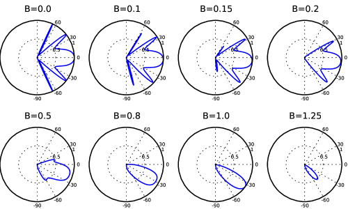
Figure 2: Transmision through a single electrostatic barrier of width 100nm and height 180meV with a varying magnetic field across the 100nm barrier region. Incident energy is 82.66 meV

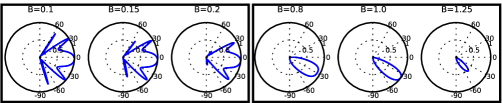
Figure 3: Transmission through a single electrostatic barrier of width 100nm and height 180meV with a varying magnetic field across the 100nm barrier region. Incident energy is 82.66 meV. Left: Results calculated using asymptotic form of parabolic cylindrical functions valid at low magnetic fields. Right: Results calculated using parabolic cylindirical functions valid at high magnetic fields. Comparison with Fig. 2 shows that both in the high as well as low magnetic field limit results can be reproduced by the current method very accurately.

5.3 Gaussian Barrier

We consider a single gaussian-shaped magnetic field barrier with no electrostatic field and compute the transmission by using a coarse and a fine piecewise approximation. In the coarse approximation, it is reduced to a a single square barrier and the fine approximation consists of it being approximated by as a series of barriers of varying height. The two approximations are shown in Figure 4. The $1/e$ width of the gaussian curve is 140nm and the peak magnetic field is 1T. The coarse approximation consists of a single barrier of width 140nm and magnetic field $\pi/2$ T. The fine approximation consists of the division of the gaussian barrier into 21 slices with a maximum field variation of not more than 0.1T taken to be constant. The incident energy is 82.66 meV. The two transmission plots are also shown. This example clearly demonstrates the utility of being able to perform computations for low magnetic fields even if the peak field value is high.

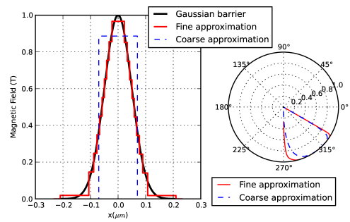
Figure 4: A gaussian shaped magnetic barrier with two different approximations. (a) The gaussian curve with the coarse and fine approximations (b) Transmission plots for both approximations

5.4 Experimental Data

We calculate the transmission in graphene based on the experimental data given in [33]. They have shown that the presence of disorder in graphene gives rise to localised charge distributions on the surface, or as they are called, electron and hole puddles. They have also measured this charge distribution. It is known that a scalar potential applied to graphene sheet shifts the Dirac point and leads to charge accumulation. We therefore model the charge as arising from a scalar potential distribution proportional to it. We have calculated the transmission corresponding to a one-dimensional potential extracted from their experimental data scaled by an arbitrary factor of $10^{-29}$. The scalar potential and the transmission data are shown in Figure 5.

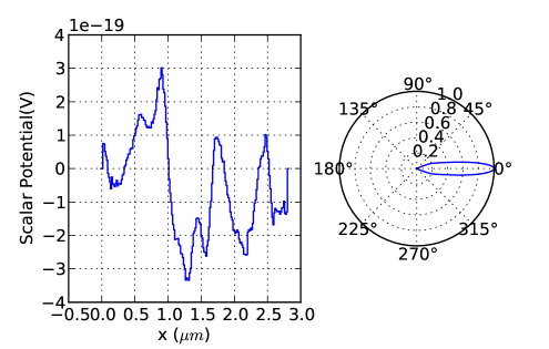
Figure 5: Scalar potential distribution from experimental data given in [33] and the corresponding transmission.

5.5 Random magnetic fields

It has been shown that any elastic deformation in the graphene sheet manifests itself as effective gauge fields acting on charge carriers[34]. This can be caused by a corrugated substrate or by the intrinsic thermodynamic ripples in graphene. It has also been shown that several electronic devices can be built by controlling the strain.[35].

The relation between a strain field and gauge fields is given in [34]. For a strain field with tensor components $u_{xx}$ and $u_{yy}$ denoting the normal strain and $u_{xy}$ the shear strain, the relation to scalar and vector potentials is as follows ($\beta,t,a,c,g$ are constants)

$$A_{x} =c\frac{\beta t}{a}(u_{xx}-u{yy})$$

$$A_{y} =-c\frac{\beta t}{a}u_{xy}$$

$$V =g(u_{xx}+u{yy})$$

Therefore, a strain field can be modelled as a gauge field. In the special case that only x-dependent shear strain is present, the only component of the equivalent magnetic field is $A_{y}(x)$ which is a Landau gauge representable vector potential.

We carry out a transmission calculation in the presence of disorder with the magnetic field and scalar potential chosen randomly. Fifty slices, each 10 nm wide are taken with the magnetic field in each slice uniformly distributed between -1 T and 1 T. The scalar potential in each slice is uniformly distributed between 0 and 200meV. A typical result is given in Figure 6, where the magnetic field, scalar and vector potentials are shown alongwith the resultant transmission.

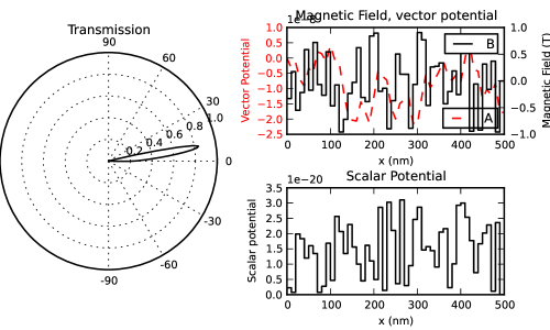
Figure 6: Computation with random fields. (a) Transmission plot (b) Magnetic Field and vector potential (c) Scalar potential

5.6 Application to bilayer graphene

This series technique can also be extended to bilayer graphene in the presence of electrostatic and magnetic fields to obtain the transmission at high energies and low magnetic fields. This method has been used in a recent communication [36].

6 Conclusion

We have applied the transfer matrix method to solve transmission problems in graphene in the presence of inhomogeneous electric and magnetic fields. We have brought out some of the difficulties associated with parabolic cylindrical functions and proposed a method to get around its limitations by changing the basis functions to a series solution which tends to complex exponentials. Despite the overhead of numerically computing a series sum, our method is robust and easy to implement with different cases not needing separate treatment compared to the use of parabolic cylindrical functions with or without asymptotic expansions. We also believe that the method is quite general and can be profitably employed whenever the wave equation is being solved with the transfer matrix method.

7 Acknowledgments

This work is supported by grant SR/S2/CMP-0024/2009 by Science and Engineering Research Council, DST, Govt. of India.

References

- [1] A K Geim and K S Novoselov. The rise of graphene. Nature materials, 6(3):183–191, March 2007.
- [2] A K Geim. Graphene: status and prospects. Science (New York, N.Y.), 324(5934):1530–1534, June 2009.
- [3] a. Castro Neto, F. Guinea, N. Peres, K. Novoselov, and a. Geim. The electronic properties of graphene. Reviews of Modern Physics, 81(1):109–162, January 2009.
- [4] N. Peres. Colloquium: The transport properties of graphene: An introduction. Reviews of Modern Physics, 82(3):2673–2700, September 2010.
- [5] M. I. Katsnelson, K. S. Novoselov, and a. K. Geim. Chiral tunnelling and the Klein paradox in graphene. Nature Physics, 2(9):620–625, August 2006.
- [6] A. De Martino, L. Dell’Anna, and R. Egger. Magnetic Confinement of Massless Dirac Fermions in Graphene. Physical Review Letters, 98(6):066802, February 2007.
- [7] A. De Martino, L Dellanna, and R Egger. Magnetic barriers and confinement of Dirac‚ÄìWeyl quasiparticles in graphene. Solid State Communications, 144(12):547–550, December 2007.
- [8] A. Ghatak, K. Thyagarajan, and M. Shenoy. Numerical analysis of planar optical waveguides using matrix approach. Journal of Lightwave Technology, 5(5):660–667, 1987.
- [9] B. Jonsson and S.T. Eng. Solving the Schrodinger equation in arbitrary quantum-well potential profiles using the transfer matrix method. IEEE Journal of Quantum Electronics, 26(11):2025–2035, 1990.
- [10] Petarpa Boonserm. Rigorous bounds on Transmission, Reflection, and Bogoliubov coefficients. PhD thesis, Victoria University of Wellington, June 2009.
- [11] P Boonserm and M Visser. One Dimensional Scattering Problems : A Pedagogical Presentation of the Relationship between Reflection and Transmission Amplitudes. Thai Journal of Mathematics, 8:83–97, 2010.
- [12] Sina Khorasani and A L I Adibi. Analytical solution of linear ordinary differential equations by differential transfer matrix method. Electronic Journal of Differential Equations, 79:1–18, 2003.
- [13] M. Ramezani Masir, P. Vasilopoulos, a. Matulis, and F. Peeters. Direction-dependent tunneling through nanostructured magnetic barriers in graphene. Physical Review B, 77(23):235443, June 2008.
- [14] Michaël Barbier, P. Vasilopoulos, F. Peeters, and J. Pereira. Bilayer graphene with single and multiple electrostatic barriers: Band structure and transmission. Physical Review B, 79(15):155402, April 2009.
- [15] M Ramezani Masir, P Vasilopoulos, and F M Peeters. Kronig-Penney model of scalar and vector potentials in graphene. Journal of physics. Condensed matter, 22(46):465302, November 2010.
- [16] Yu-Xian Li. Transport in a magnetic field modulated graphene superlattice. Journal of Physics: Condensed Matter, 22(1):015302, January 2010.
- [17] Lifeng Sun, Chao Fang, Yu Song, and Yong Guo. Transport properties through graphene-based fractal and periodic magnetic barriers. Journal of Physics: Condensed Matter, 22:445303, 2010.
- [18] M. Ramezani Masir, P. Vasilopoulos, and F. Peeters. Fabry-Pérot resonances in graphene microstructures: Influence of a magnetic field. Physical Review B, 82(11):115417, September 2010.
- [19] A. F. Young and F. Kim. Electronic Transport in Graphene Heterostructure. Annual Reviews of Condensed Matter Physics, 2:101, November 2011.
- [20] Godfrey Gumbs. Relativistic scattering states for a finite chain with -function potentials of arbitrary position and strength. Physical Review A, 32(2):1208–1210, August 1985.
- [21] Sankalpa Ghosh and Manish Sharma. Electron optics with magnetic vector potential barriers in graphene. Journal of Physics: Condensed Matter, 21(29):292204, July 2009.
- [22] Wayne W Lui and Masao Fukuma. Exact solution of the Schrodinger equation across an arbitrary one-dimensional piecewise-linear potential barrier. Journal of Applied Physics, 60(September):1555–1559, 1986.
- [23] L. Oroszlány, P. Rakyta, a. Kormányos, C. Lambert, and J. Cserti. Theory of snake states in graphene. Physical Review B, 77(8):081403(R), February 2008.
- [24] Shanjie Zhang and Jianming Jin. Computation of Special Functions. John Wiley and Sons, NY, 1996.
- [25] N.M. Temme. Numerical and asymptotic aspects of parabolic cylinder functions. Journal of computational and applied mathematics, 121(1-2):221–246, 2000.
- [26] Nico M Temme. Numerical and Asymptotic Aspects of Parabolic Cylinder Functions. arXiv:math/0109188v1, September 2001.
- [27] L. Dell’Anna and a. De Martino. Wave-vector-dependent spin filtering and spin transport through magnetic barriers in graphene. Physical Review B, 80(15):155416, October 2009.
- [28] Luca Dell’Anna and Alessandro De Martino. Magnetic superlattice and finite-energy dirac points in graphene. Phys. Rev. B, 83(15):155449, Apr 2011.
- [29] G.N. Watson. The Harmonic Functions Associated with the Parabolic Cylinder. Proc. London Math. Soc, s2-8:393–421, 1910.
- [30] Nathan Schwid. The Asymptotic Forms of the Hermite and Weber Functions. Transactions of the American Mathematical Society, 37(2):339–362, March 1935.
- [31] George B Arfken and Hans J Weber. Mathematical Methods for Physicists. Academic Press, 2001.
- [32] William H. Press and Brian P. Flannery. Numerical Recipes in C: The art of scientific computing. Cambridge University Press, 1992.
- [33] J. Martin, N. Akerman, G. Ulbricht, T. Lohmann, J. H. Smet, K. von Klitzing, and a. Yacoby. Observation of electron‚Äìhole puddles in graphene using a scanning single-electron transistor. Nature Physics, 4(2):144–148, November 2008.
- [34] F. Guinea, Baruch Horovitz, and P. Le Doussal. Gauge fields, ripples and wrinkles in graphene layers. Solid State Communications, 149(27-28):1140–1143, July 2009.
- [35] Vitor Pereira and a. Castro Neto. Strain Engineering of Graphene’s Electronic Structure. Physical Review Letters, 103(4):046801, July 2009.
- [36] Neetu Agrawal, Sameer Grover, Sankalpa Ghosh, and Manish Sharma. Reversal of Klein reflection in bilayer graphene. Journal of Physics: Condensed Matter, 24(17):175003, April 2012.