Convolutions power of a characteristic function

Abstract

This paper deals with the convolution powers of the characteristic function of $[0,1],\chi_{[0,1]}$ and its function-derivatives. The importance that such convolution products have can be seen, for an instance, at [2] where there is the need to find the best differentiable splines as regularization tool to be used to expand functions or in the spectral analysis of signals. Another simple application of these convolution powers is in the construction of a partition of the unity of a very high class of differentiability. Here, some properties of these convolution powers have been obtained which easily led to write the algorithm to produce convolution powers of $\chi_{[0,1]}$ and their function-derivatives. This algorithm was written in calc, the program published under GPL that is free to download.

key words:  convolution power, b-splines,compact support, GPL .

MSC: Primary 65D07, Secondary 65D15

1 Introduction

The $n$-th convolution power of the characteristic function of an interval is an $(n-1)$-b-splines, this is the subject of this paper. This first section will be a general description of the work done, the notation used, finishing with three lemmas and a theorem, which are the main tools used in this work.

Then we proceed in section 2 with the calculus of the powers 2,3,4 in a way to uncover the recursion which will be finally clear in the calculus of the third power. The forth power will be a preparation for the final theorem (algorithm) which will be presented at the section 3. The section 2 is, thus, preparatory for the proof at section 3, and was thought to permit the reader to construct the algorithm for himself, so the reader can skip to the section 3, if he find that this subject is familiar and if he want only to see the main result.

In the section 4 it will be presented a computer program which is a machine translation of the theorem stated at section 3. Finally, the last section, contains some applications suggested for the material in this paper and a characterization of a general space of univariated splines.

We have used calc [3], a computer language specialized to construct mathematical algorithms with infinite precision this meaning that it can deals with arbitrarily long integers which is fundamental to this work as it will be necessary to use factorial for any value of $n$ in the calculus of the convolution powers. In section 4 you can see a graphic output of the program for $n=30$.

1.1 Some history

Splines are pieces of polynomials pasted together in conditions to make a continuous, and even more, a highly differentiable function. In the last section you may find a definition for a class of splines. It is a simple idea which turned into a very powerful tool in such diverse areas as geometric design or approximation theory. In the background there is a famous theorem of Weierstrass stating that any continuous function can be arbitrarily approximated by polynomials. There was a huge work to make this simple and easy, and we can consider a bad example the Taylor polynomials, which make a very good approximation of a function in a sole point but which is good enough to be used to approximate periodic functions like sine. The bad thing with classical polynomial approximation is that computers do not like it that much because it needs a very high degree to get something useful. You can remember Lagrange polynomial interpolation which does a good job if the points to be linked together are not jumping to much and the critical situation is at the boundary of the interval which defines the region where the points have been selected. This is a particular problem to classical polynomial approximation because just around the boundary of the region containing its roots a polynomial will behave wildly. If you have selected $n$ points the corresponding Lagrange polynomial is of degree $n-1$.

Then splines came out to be the solution. With some pieces of first degree polynomials you may have a very good approximation of data collected from a sensor, provided that you are only interested in the total amount of the phenomenon, its integral. Well this was the trick, paste together several piece of polynomials instead of a unique monolithic polynomial as a Lagrange polynomials. The piecewise first degree polynomials are 1-splines, known as polygonal lines.

Switching to polynomials of second degree we can already have a better approximation and the famous algorithm of Runge-Kutta does exactly this for solving differential equations, though not with splines. But degree two polynomials have a big lack of flexibility since they do not provide a change of convexity in each piece, they are 2-splines. So, the next step is to paste together pieces of polynomials of third degree and this has proved to be a good solution for a large number of problems needing polynomial approximation: 3-splines.

At this point it should pop up a definition for this little thing called splines that started to be used in the seventies and today is a very big network of research in Mathematics. To be an $n$-splines, the pieces of polynomial should be of degree less or equal to $n$, there can be a straight line infiltrated in the business. The second condition is that the resulting function has to be of class $C^{n-1}$.

It is simple like that but the main literature about splines, for example, the historic book of Larry Schumaker [5], is not easy to be read though it is at the beginning of the history. This is the point with this paper, it is starting by the end, not from the beginning, and there are some powerful tools that had been added to the history to make splines easy.

1.2 The contribution of this paper

In chapter 6 of [1], the author has shown that the n-th convolution power of the characteristic function of the interval $[0,1]$ is an $(n-1)$-splines having as support the interval $[0,n]$ and he starts by showing that the convolution of two characteristic functions results in a 1-splines. Here you are the basic tool to build splines: the convolution. Convolution is a “multiplication”, it satisfies the distributive law relatively to the sum, hence a sum of characteristic functions of intervals can be multiplied by a selected characteristic function of an interval, using convolution, to produce a 1-splines. Iterating this process you will reach an n-splines for the desired $n$. But this take a lot of time and computer power and the alternative is to construct a splines-bases to generate an appropriate space of splines and this is the tool that this paper is going to produce: an approximate unity to build up bases for vector spaces of splines. This is an well known application that will be only mentioned at the last section as complement to the main result of this paper. These convolution powers can be easily be transformed into a sharp approximate unity with respect to the convolution product and this will be mentioned again at section 5.

Here we have a slightly different methodology from the one at [1], besides presenting four properties of $f=(\chi_{[0,1]})^{n}$, which are the lemmas and the theorem at section 2, the work is directed to a recursive program that is able to produce the whole formula not only of $f=(\chi_{[0,1]})^{n}$ but for all its function-derivatives, having as input the power $n$ which is needed. This is the main result of the paper, theorem 4, in the section 3 followed by the correspondent algorithm, a computer program, in section 4. The program produces functions for gnuplot [7], which may be run to show the graphics of $f$ and is able to write the matrix of the coefficients of $f$ and all its function-derivatives.

There are recent works, see [2] for example, which show the importance of convolutions in “spectral analysis” mainly in the context of wavelets. This is an example of the importance of having a simple way to present convolution powers and a good algorithm to produce them. This paper offers that contribution in this matter in the particular case of convolution of characteristic functions of intervals of the line.

The whole construction is done step by step, in a way to permit the reader to construct by himself the method.

Our main motivation with this paper is the construction of a tool to be used in the analysis of differential operators and in the spectral analysis of wavelet and we think this is underway.

2 The convolution powers of $\chi$

In this section, first, we introduce the notation and basic results necessary to proof the main theorem of the paper, following this we are going to calculate the powers 2, 3, 4, in order to formulate the general result.

2.1 Basic results

Here you are the basic notation that will be stated together with three Lemmas which are the underground tools for the theorems of the paper.

The characteristic function of the interval $[0,1]$ will be refereed to using one of the following notations:

$$\chi_{0}=\chi_{[0,1]}=\chi$$ (1)

It will be used the index when necessary to indicate a translation of $a\in\mathbf{R}$, then

$$\chi_{a}(x)=\chi_{0}(x-a)=\chi(x-a);$$ (2)

The use power notation for “convolution power” has no risk of possible confusion with the “arithmetic power”, since the context will indicate what is the meaning in the few occasions in which the “arithmetic power” will be used. Hence $\chi=\chi^{1}$ is the first power, as usual, and we can add a sense to $\chi^{0}$ as the constant function.

The symbol $f=\chi^{n}$ will be used to simplify the notation of the $n$-th convolution power, which is the main goal of this paper, hence $f$ do represent the $n$-th convolution power of $\chi$, consistently, in the whole paper.

The second convolution power of the characteristic function is the triangle function, a 1-splines, whose derivative is the the difference of two the translations of the characteristic function: $\chi_{0}-\chi_{1}$. This is a consequence of the following lemmas.

Lemma 1 (Convolution and derivative)

$$\frac{d}{dx}(f*g)=\frac{df}{dx}*g=f*\frac{dg}{dx}$$

Lemma 2 (Distribution derivative of characteristic function)

$$\frac{d\chi}{dx}=\delta_{0}-\delta_{1}$$

Lemma 3 (Convolution with $\delta_{a}$ and translation)

$$(\delta_{a}*f)(x)=f(x-a)$$

Using these lemmas it can be proved:

Theorem 1 (Derivative of the second convolution power)

If

$$f=\chi*\chi=\chi^{2}$$

then

$$f^{\prime}=\chi_{0}-\chi_{1}$$

In lemma 3, when the translation parameter is $a=0$, we can see that the Dirac delta measure is the unity of convolution as an element of an extension ring of the convolution ring of functions which does not have a unity.

2.2 The second convolution power

These three properties stated as lemmas produce an easy way to get the second convolution power of $\chi$, the above mentioned triangle function, (compare with the heavy work at [1, chapter 6]. Moreover, this method will be used all along the paper, repeatedly, the main reason being that we shall have a succession of integrals whose domains of integration are disjoints, they coincide, in fact, exactly on a single point.

$$f^{\prime}=(\chi*\chi)^{{}^{\prime}}=\chi*\chi^{{}^{\prime}}=\chi*(\delta_{0}-\delta_{1})$$ (3)

$$f^{\prime}=(\chi*\chi)^{{}^{\prime}}=\chi*\delta_{0}-\chi_{0}*\delta_{1}$$ (4)

$$f^{\prime}=(\chi*\chi)^{{}^{\prime}}=\chi-\chi_{1}$$ (5)

$$f(x)=\chi*\chi(x)=\chi^{2}(x)=\int\limits_{0}^{x}\left(\chi(t)-\chi_{1}(t)\right)dt$$ (6)

$$f(x)=\chi^{2}(x)=\left\{\begin{array}[]{ll}x<0&0\\ x\in[0,1]&\int\limits_{0}^{x}dt\\ x\in[1,2]&a-\int\limits_{1}^{x}\chi_{1}(t)dt\\ x>2&0\\ \end{array}\right.$$ (11)

$$f(x)=\chi^{2}(x)=\left\{\begin{array}[]{ll}x<0&0\\ x\in[0,1]&x\\ x\in[1,2]&1-\int\limits_{0}^{x-1}dt\\ x>2&0\\ \end{array}\right.$$ (16)

$$f(x)=\chi^{2}(x)=\left\{\begin{array}[]{ll}x<0&0\\ x\in[0,1]&x\\ x\in[1,2]&1-(x-1)\\ x>2&0\\ \end{array}\right.$$ (21)

and now it is easy to see that $\chi^{2}$ is the so called triangle function centered at 1 with support $[0,2]$ and height $1$ at 1. You may observe the presence of the symbol “$a$”, at equation (7), which is the value of the integral on $[0,1]$ and is the initial condition of the integral on $[1,2]$. This trend will be repeated further and further for all convolution powers. The symbols “$a,b,c,\ldots$”, will be used temporally, before their values can be expressed.

The triangle function can be defined as $\chi^{2}(x)=x\chi+(2-x)\chi_{1}$. This expression is not useful in computations, but it will be of good help in the mathematical formulation, in the logic preparation which will produce the algorithm.

Observe that the (distribution) derivative of $\chi$ is $\delta_{0}-\delta_{1}$ where $\delta_{a}$ is the Dirac measure concentrated at the point $a$. The fact that the “convolution with the Dirac measure is a translation of the other convolution factor” has been used in equation (5).

An easy and beautiful theorem, extending theorem 1, can be stated, immediately.

Theorem 2 (Derivative of $f$)

the $n$-th convolution power

$$\frac{d}{dx}f(x)=\frac{d}{dx}\chi^{n}(x)=\chi^{n-1}(x)-\chi_{1}^{n-1}(x)$$ (22)

the derivative of a convolution power $f$ of $\chi$ is the difference of translates of the previous power. The proof is a direct application of Lemmas 1, 2 and 3. This theorem will be used several times in the sequence.

A notation will be introduced to simplify the expression of $f$. Put $P_{1}(x)=x$ then the equation (9) reads:

$$f(x)=\chi^{2}(x)=\left\{\begin{array}[]{ll}x<0&0\\ x\in[0,1]&P_{1}(x)\\ x\in[1,2]&1-P_{1}(x-1)\\ x>2&0\\ \end{array}\right.$$ (23)

Observe that the second convolution power has been defined in terms of a linear combination of a polynomial of degree one and its translates (the plural will be valid in a near future…), this highlights that $f$, the second convolution power, is 1-b-splines as particular case of the first sentence of the paper, that “$n$-th convolution power is an $(n-1)$-b-splines”. It will be possible to go further using this kind of polynomials and the same will be done with the next power so to make clear the recursion of the process.

2.3 The third convolution power

Before going ahead let us stress that the whole secret is contained in first calculating the derivatives of the next power which we already have, thinking that, to calculate the next power first we must have the previous one…So let’s calculate the derivatives of the third convolution power to have:

$$\frac{df}{dx}=\frac{d}{dx}\chi^{3}(x)=\chi^{2}(x)-\chi^{2}(x-1)$$ (24)

$$\frac{d^{2}f}{dx^{2}}=\frac{d^{2}}{dx^{2}}\chi^{3}(x)=\chi(x)-2\chi(x-1)+\chi(x-2);$$ (25)

where we can see the binomial coefficients: 1,-2,1 as usual when calculating derivatives of products and, here, there is a “difference” in the “game”.

This suggests, by the way, another beautiful and easy theorem:

Theorem 3 (The $n-1$ derivative)

of the $n$ convolution power

1. The $n$-th convolution power, $f=\chi^{n}$, is an $(n-1)$-b-splines of compact support $[0,n]$, hence $f$ has $n-1$ function-derivatives of whose $n-2$ are continuous.

2. The derivative of order $n-1$ of the $n$-th convolution power $f$, which is not continuous, is given by the linear combination of translates of $\chi$

   $$\frac{d^{(n-1)}f}{dx^{(n-1)}}=\sum\limits_{k=0}^{n-1}(-1)^{k}(^{n-1}_{k})\chi_{k}$$

The coefficients of this linear combination are the elements of the line of order $n-1$ of the “alternate Pascal Triangle”, these elements are the coefficients of $(x-1)^{n-1}$, (the line of order zero has only one element, 1).

The proof comes by recursion with repeated application of the lemmas 1, 2, 3 and theorem 1.

The calculus of the iterated integral of $f^{\prime\prime}$ will be easy as it is again a succession of integrals whose integration domains are disjoints (coincide on a set of measure zero), one point set.

Hence the third convolution power is twice the integral of its second derivative starting at the initial condition $x=0$. We know in advance that the support of this convolution is $[0,3]$, from [1], and that there will be different equations each time we go over an integer boundary. The initial condition of each integral is the total value of the previous integral to make a continuous function. This will be represented by the symbols $a,b$, temporally.

In condition to obtain the recursion formula, it is necessary to introduce here a rather complicated notation, but intuitive, indeed. It will protect the parts of the expression which will pop up. Observe that the second derivative of the third convolution power is not continuous as a linear combination of translations of $\chi$ with coefficients being the alternate binomial numbers, as in the powers of (x-1). So let the following numbers be defined:

$$\left\{\begin{array}[]{l}Bin(n,k)=(-1)^{k}(^{n}_{k})\\ a_{00}=Bin(2,0);\\ a_{01}=Bin(2,1);\\ a_{02}=Bin(2,2);\\ \end{array}\right.$$ (26)

With this notation it may be written

$$\frac{d^{2}f}{dx^{2}}=\frac{d^{2}}{dx^{2}}\chi^{3}=f^{\prime\prime}(x)=\left\{\begin{array}[]{ll}x<0&0\\ x\leq 1&a_{00}\chi(x)\\ x\leq 2&a_{01}\chi(x-1)\\ x\leq 3&a_{02}\chi(x-2)\\ x>3&0\\ \end{array}\right.$$ (27)

Integrating twice this second derivative we shall obtain the formulation of $f$. At this point, $f$ is the second convolution power of $\chi$. A new set of coefficients will be defined in the run and, for a while, the convention, state previously, to use the symbols $a,b$ as the initial conditions for the second and third integrals, will be used.

$$f^{\prime}(x)=\int_{0}^{x}\left(a_{00}\chi(t)+a_{01}\chi(t-1)+a_{02}\chi(t-2)\right)dt$$ (28)

$$f^{\prime}(x)=\left\{\begin{array}[]{ll}x<0&0\\ x\leq 1&a_{00}x\\ x\leq 2&a+a_{01}\int_{1}^{x}\chi(t-1)dt\\ x\leq 3&b+a_{02}\int_{2}^{x}\chi(t-2)dt\\ x>3&0\\ \end{array}\right.$$ (34)

$$f^{\prime}(x)=\left\{\begin{array}[]{ll}x<0&0\\ x\leq 1&a_{00}x\\ x\leq 2&a+a_{01}\int_{0}^{x-1}\chi(t)dt\\ x\leq 3&b+a_{02}\int_{0}^{x-2}\chi(t)dt\\ x>3&0\\ \end{array}\right.$$ (40)

$$f^{\prime}(x)=\left\{\begin{array}[]{ll}x<0&0\\ x\leq 1&a_{00}x\\ x\leq 2&a_{00}+a_{01}(x-1)\\ x\leq 3&a_{00}+a_{01}+a_{02}(x-2)\\ x>3&0\\ \end{array}\right.$$ (46)

$$f^{\prime}(x)=\left\{\begin{array}[]{ll}x<0&0\\ x\leq 1&a_{10}x\\ x\leq 2&a_{11}+a_{01}(x-1)\\ x\leq 3&a_{12}+a_{02}(x-2)\\ x>3&0\\ \end{array}\right.$$ (52)

$$\left\{\begin{array}[]{ll}a_{10}=&a_{00};\\ a_{11}=&a_{10}P_{1}(1);\\ a_{12}=&a_{11}+a_{01}P_{1}(1);\\ \end{array}\right.$$ (56)

The equation (33) can be written a bit different in a way to show that the sum of certain indexes is constant in each row. This rule is valid with two exceptions which are meaningless to the definition of the algorithm:

1. The first row of the matrix $a_{0j}=Bin(n,j)$;

2. The two first elements in in each row

   $$a_{i0}=a_{00};a_{i1}=a_{i0}=a_{00}$$

$$\left\{\begin{array}[]{ll}a_{10}=&a_{00}P_{1}(1);\\ a_{11}=&a_{10}P_{0}(1);\\ a_{12}=&a_{11}P_{0}(1)+a_{01}P_{1}(1);\\ \end{array}\right.$$ (57)

In equation (57) it is being used the family of polynomials

$$P_{k}(x)=x^{k}/k!;$$ (58)

In the equations to define the coefficients $a_{ij}$ we have in each row a sum of products $a_{ij}P_{k}(1)$ and the sum $i+k$ is the order of the row when $j\geq 2$ (the above mentioned exception).

To obtain a new row $a_{ij}$, we have to use all the possibilities in “$i+k=$order of the row”. This law will be valid in the sequence.

Calculating the next integral we shall have:

$$f(x)=\left\{\begin{array}[]{ll}x<0&0\\ x\leq 1&a_{10}\int\limits_{0}^{x}tdt\\ x\leq 2&a+a_{11}\int\limits_{1}^{x}dt+a_{01}\int\limits_{1}^{x}(t-1)dt\\ x\leq 3&b+a_{12}\int\limits_{2}^{x}dt+a_{02}\int\limits_{2}^{x}(t-2)dt\\ x>3&0\\ \end{array}\right.$$ (64)

$$f(x)=\left\{\begin{array}[]{ll}x<0&0\\ x\leq 1&a_{10}P_{2}(x)\\ x\leq 2&a_{10}P_{2}(1)+a_{11}\int\limits_{0}^{x-1}dt+a_{01}\int\limits_{0}^{x-1}tdt\\ x\leq 3&b+a_{12}\int\limits_{0}^{x-2}dt+a_{02}\int\limits_{0}^{x-2}tdt\\ x>3&0\\ \end{array}\right.$$ (70)

$$f(x)=\left\{\begin{array}[]{ll}x<0&0\\ x\leq 1&a_{20}P_{2}(x)\\ x\leq 2&a_{20}P_{2}(1)+a_{11}P_{1}(x-1)+a_{01}P_{2}(x-1)\\ x\leq 3&b+a_{12}P_{1}(x-2)+a_{02}P_{2}(x-2)\\ x>3&0\\ \end{array}\right.$$ (76)

$$f(x)=\left\{\begin{array}[]{ll}x<0&0\\ x\leq 1&a_{20}P_{2}(x)\\ x\leq 2&a_{20}P_{2}(1)+a_{11}P_{1}(x-1)+a_{01}P_{2}(x-1)\\ x\leq 3&a_{20}P_{2}(1)+a_{11}P_{1}(1)+a_{01}P_{2}(1)+a_{12}P_{1}(x-2)+a_{02}P_{2}(x-2)\\ x>3&0\\ \end{array}\right.$$ (82)

$$f(x)=\left\{\begin{array}[]{ll}x<0&0\\ x\leq 1&a_{20}P_{2}(x)\\ x\leq 2&a_{21}P_{2}(1)+a_{11}P_{1}(x-1)+a_{01}P_{2}(x-1)\\ x\leq 3&a_{22}+a_{12}P_{1}(x-2)+a_{02}P_{2}(x-2)\\ x>3&0\\ \end{array}\right.$$ (88)

Some remarks here will make things clear in the next step. In equation (59) the symbols $a,b$ have been used as explained before, and in equation (60) the limits of integration have been changed accordingly with the interval of definition, and the liberty of translation invariance of Lebesgue measure has been used to change the limits of $\int\limits_{0}^{x-2}dt$ in conditions to have the same setting in both integrals. This leads to a translation of the polynomial $P_{i}$, naturally. This will be further commented in a moment. The symbol $a$ has been evaluated as $f(1)$ and the symbol $b$ has been evaluated as

$$b=f(2)=a_{21}P_{2}(1)+a_{11}P_{1}(1)+a_{01}P_{2}(1)$$

the value of the primitive over $[1,2]$ evaluated at point $x=2$. On the interval $[2,3]$ it can be written $a_{22}P_{0}(x-2)$ to enhance the property

$$a_{mj}P_{i}(x-k);m+i=j$$

where $j$ is the order of the row. The new set of coefficients will be defined explicitly:

$$\left\{\begin{array}[]{ll}a_{20}&=a_{10}=a_{00};\\ a_{21}&=a_{20}P_{2}(1);\\ a_{22}&=a_{21}P_{0}(1)+a_{11}P_{1}(1)+a_{01}P_{2}(1);\\ \end{array}\right.$$ (90)

and remember the exception to the rule that the first two coefficients in each row have a particular law. With these definitions $f$ is

$$f(x)=\left\{\begin{array}[]{ll}x<0&0\\ x\leq 1&a_{20}P_{2}(x);\\ x\leq 2&a_{21}P_{0}(x-1)+a_{11}P_{1}(x-1)+a_{01}P_{2}(x-1)\\ x\leq 3&a_{22}P_{0}(x-2)+a_{12}P_{1}(x-2)+a_{02}P_{2}(x-2)\\ x>3&0\\ \end{array}\right.\\$$ (91)

a linear combination of the elements of last row of the matrix $a[i,j]$ with translations of all the polynomials $P_{k};k=0,\ldots,n$, where $n+1$ is the desired convolution power. The previous raws of this matrix give the derivatives of $f$ but the summations are being restricted of one unity in each further derivative. This will be clear in the last section, but you can conclude from the above calculations that:

$$f^{\prime}(x)=\left\{\begin{array}[]{ll}x<0&0\\ x\leq 1&a_{10}P_{1}(x);\\ x\leq 2&a_{11}P_{0}(x-1)+a_{01}P_{1}(x-1)\\ x\leq 3&a_{12}P_{0}(x-2)+a_{02}P_{1}(x-2)\\ x>3&0\\ \end{array}\right.$$ (97)

$$f^{\prime\prime}(x)=\left\{\begin{array}[]{ll}x<0&0\\ x\leq 1&a_{00}P_{0}(x);\\ x\leq 2&a_{01}P_{0}(x-1)\\ x\leq 3&a_{02}P_{0}(x-2)\\ x>3&0\\ \end{array}\right.$$ (103)

Remark that $P_{0}$ can be replaced by $\chi$, but this is of no help at all.

2.4 The forth convolution power

From this point the recurrence is established:

1. The convention for indexes follows the syntax of the language ${\mathtt{C}}^{++}$ for which the first positive (integer) index is zero, this way in a $n\times n$ matrix the indexes run from $0\ldots n-1$. The matrix $(a_{ij});i,j=0,\cdots,n-1$ where $n$ is the desired power;

2. to use the entries in the last row of this matrix to define $f(x)$ as combinations of translations of $P_{i}(x),P_{i}(x-k),$ to the interval $[k,k+1]$.

3. The $n-1$ derivatives of $f$ are obtained, from the raw $n-2$ to the raw zero with increasing order of derivation and decreasing the number of summations of powers of $P_{i}$ in the same way as $f$.

4. The starting point is the derivative of order $n-1$ which comes from the line of order $n-1$ of the alternate Pascal triangle.

The forth power, $f$, of $\chi$ may, now, be written, directly, without further integrations as an example before writing the algorithm formally.

By Theorem 2, $f$ has tree derivatives, two continuous derivatives, it is 3-splines. So the algorithm will start from the line of order 3 of the “alternate” Pascal triangle:

$$a_{0k}=Bin(3,k);k=0\dots 3;$$ (104)

$$\left\{\begin{array}[]{ll}a_{10}&=a_{00};\\ a_{11}&=a_{10}P_{1}(1);\\ a_{12}&=a_{11}P_{0}(1)+a_{01}P_{1}(1);\\ a_{13}&=a_{12}P_{0}(1)+a_{02}P_{1}(1);\\ \end{array}\right.$$ (109)

$$\left\{\begin{array}[]{ll}a_{20}&=a_{00}P_{0}(1)\\ a_{21}&=a_{20}P_{2}(1);\\ a_{22}&=a_{21}P_{0}(1)+a_{11}P_{1}(1)+a_{01}P_{2}(1);\\ a_{23}&=a_{22}P_{0}(1)+a_{12}P_{1}(1)+a_{02}P_{2}(1);\\ \end{array}\right.$$ (114)

$$\left\{\begin{array}[]{ll}a_{30}&=a_{00}P_{0}(1)\\ a_{31}&=a_{30}P_{3}(1);\\ a_{32}&=a_{31}P_{0}(1)+a_{21}P_{1}(1)+a_{11}P_{2}(1)+a_{01}P_{3}(1);\\ a_{33}&=a_{32}P_{0}(1)+a_{22}P_{1}(1)+a_{12}P_{2}(1)+a_{02}P_{3}(1);\\ \end{array}\right.$$ (119)

and

$$f(x)=\left\{\begin{array}[]{ll}x<0&0\\ x<1&a_{30}P_{3}(x);\\ x<2&a_{31}P_{0}(x-1)+a_{21}P_{1}(x-1)+a_{11}P_{2}(x-1)+a_{01}P_{3}(x-1)\\ x<3&a_{32}P_{0}(x-2)+a_{22}P_{1}(x-2)+a_{12}P_{2}(x-2)+a_{02}P_{3}(x-2)\\ x<4&a_{33}P_{0}(x-3)+a_{23}P_{1}(x-3)+a_{13}P_{2}(x-3)+a_{03}P_{3}(x-3)\\ x>4&0\\ \end{array}\right.$$ (120)

Observe that by Theorem 1 the derivatives of $f$ can be traced back by difference of translations of the previous powers up to the last function-derivative as a linear combination of translations of $\chi$ so we are able to right the equations of $f$ and all its function-derivatives very easily. Better said, a program can do that for us, and the program can be download from a link at [4].

3 The $n$-th convolution power

In the next theorem the indexes are separated with commas to avoid the confusion: “$n-1,1$” for “$n-11$”. The same has to be done at the program.

Theorem 4 (The $n$-convolution power)

of the characteristic $\chi_{[0,1]}$

The $n$-th convolution power of $\chi=\chi_{[0,1]}$, $f=\chi^{n}$, is $n-1$-b-splines such that

$$f(x)=\left\{\begin{array}[]{ll}0&x<0\\ a_{n-1,0}P_{n-1}(x)&x\in[0,1]\\ \sum\limits_{j=0}^{n-1}a_{n-1,j}P_{j}(x-k);k=\lceil x\rceil;&(1\leq x\leq n)\\ 0&x>n\\ \end{array}\right.$$

where the coefficients $a_{n-1,j}$ are given by the equations:

$$\left[\begin{array}[]{llllll}a_{0,0}&a_{0,1}&a_{0,2}&\cdots&a_{0,n-1}\\ a_{1,0}&a_{1,1}&a_{1,2}&\cdots&a_{1,n-1}\\ &&&\cdots&\\ a_{n-1,0}&a_{n-1,1}&a_{n-1,2}&\cdots&a_{n-1,n-1}\\ \end{array}\right]$$ (126)

$$a_{0,k}=Bin(n-1,k);k=0,\dots,n-1;Bin(n,p)=(-1)^{p}(_{p}^{n-1})$$ (127)

$$a_{1,0}=a_{0,0};$$ (128)

$$a_{1,1}=a_{1,0}P_{1}(1);$$ (129)

$$j\geq 2;j\leq n-1;a_{1,j}=a_{1,j-1}P_{1}(1);$$ (130)

$$a_{2,0}=a_{0,0}P_{0}(1);$$ (131)

$$a_{2,1}=a_{2,0}P_{1}(1);$$ (132)

$$j\geq 2;j\leq n;a_{2,j}=a_{2,j-1}+a_{1,j-1}P_{1}(1)+a_{0,j-1}P_{2}(1);$$ (133)

$$a_{3,0}=a_{0,0}P_{0}(1);$$ (134)

$$a_{3,1}=a_{3,0}P_{1}(1);$$ (135)

$$j\geq 2;j\leq n;a_{3,j}=\sum\limits_{i+k=3}b{i,j-1}P_{k}(1)$$ (136)

$$\cdots$$ (137)

$$a_{n-1,0}=a_{0,0}P_{0}(1);$$ (138)

$$a_{n-1,1}=a_{n-1,0}P_{1}(1);$$ (139)

$$j\geq 2;j\leq n-1;a_{n-1,j}=\sum\limits_{i+k=n-1}a_{i,j-1}P_{k}(1)$$ (140)

The proof:

By theorem 2, $n$-th convolution power, which is a $(n-1)$-b-splines, has $n-1$ function-derivatives, of which the first $n-2$ are continuous, and the starting point is line of order $n-1$ of the alternate Pascal triangle defined by the numbers $Bin(n-1,k)$. This is a consequence of two facts:

1. In the combination of lemmas 1 and 2 we have a relation of the type of Stifel rule, the defining relation of Pascal Triangle, modified to produce the alternate numbers $Bin(n-1,k)=(-1)^{k}(_{k}^{n-1})$. So after $n-1$ derivatives we are at line of order $n-1$ of the alternate Pascal triangle.

2. Each new derivative is a linear combination of the previous convolution power by theorem 1 so the order of convolutions power will decrease to reach order one of derivation, the non-continuous function-derivative.

This explains the first row of the $(n-1)\times(n-1)$-matrix $b[ji]$. The other rows are obtained by integrating the combination of translations of the $P_{j}$ all along of the integers of the support $[0,n]$ of $f$, and at each new integration the total variation of the previous integral is used as the initial value, with $j$ being the order of the row, $j=n-1-k$ where $k$ is the order of the derivative.

4 A computer program

There is a program written in Calc, [3], which can be download from [4], and here you are the output of the program at the figure (1)

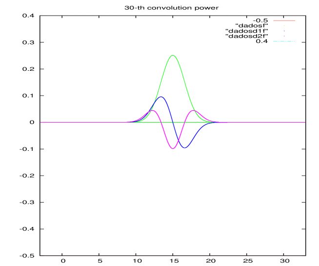
Figure 1: graphics of convolution power 30, $f,f^{\prime}f^{\prime\prime}$

for the choice of $n=30$. This is the graphic of $f,f^{\prime},f^{\prime\prime}$ when $f=\chi^{30}$. Time of this job: a few seconds.

To have the graphics of $f,f^{\prime},f^{\prime\prime}$, of course, for $n\geq 3$, do the following:

1. Start Calc, then you shall have a terminal of the calculator to make inputs. Calc is iterative, it is an interpreted language;

2. Supposing you have the code at the current directory named to

   convolution_powers.calc

   execute at the terminal of Calc:

   read convolution_powers.calc

   “execute”, means, “write the above at the terminal and hit enter”. This will make Calc learn all the functions defined at convolution_powers.calc and you shall be able to execute any of them. There is one function called main() which is written to do a big part of the job so you can have what is promised in the paper.

3. Execute “main(n)” selecting the desired value of $n$ at the terminal of Calc and you will see $f,f^{\prime},f^{\prime\prime}$. This will work out of the box, under Linux.

   You may experience some problems but then read the code and you shall see a suggestion to go around them.

4. If you want see the matrix, execute:

   • a = cria_matriz(n); either repeat the the value of n or put a new one.

   • imprime_matriz(a,n) the parameter “a” has been created in the previous step, but you still need to put the same value of $n$ as parameter. This indicates that the program is not well planned…Perhaps somebody will produce something better from this draft.

5. It is pointless to show all the $n-1$ derivatives as it will be not possible to distinguish who’s who for a large value of $n$. But, again, read the code and find a remark with the keyword “further derivatives” to see how to implement more derivatives.

5 Final remarks

As $f=\chi^{n}$ is a kernel, in the sense that it is positive and its integral is one, then it is integral preserving under convolution product. Well, this is exactly the reason why $f$ has this property because $\chi$ is a kernel. This permits to construct a partition of the unity from a set of characteristic functions associated with a partition of an interval with the desired class of differentiability. This can be done by making the convolution of $f$ with each member of this set of characteristic functions and the methodology of sections 2,3,4 of paper can be of help to produce this rapidly.

Given a kernel, in the above sense, we can transform it in a sequence which is an approximate identity, this is the terminology of [8, chapter 6, definition 6.31], the equation is $\phi_{n}=nf(nx)$. By the way, this is the expression to have a sharp kernel when constructing a partition of the unity, instead of using $f$ directly. A simple translation will produce a kernel balanced around zero, and sometimes this is interesting to have. The program presented in this paper can be easily modified to make these applications.

A simple consequence of theorem (2), applied to the an $n$-splines, show that its derivative of order $n-1$ will be a linear combination of characteristic functions of the elements of a partition of an interval of $\mathbf{R}$ (which can be the whole line). This permits a simple characterization of a quite general class of univariated splines.

Theorem 5 (Characterization)

spaces of splines

Given a partition $\Pi(I)$ of an interval $I$ of $\mathbf{R}$ (which can be the whole line), and a kernel $\phi$ being an $n$-splines of compact support

1. let’s consider $\Pi(I)$ as the index set of the characteristic functions of the intervals in $\Pi(I)$;

2. the convolutions of $\phi$ with the elements of $\Pi(I)$ are linearly independent and generate a vector space of functions of class ${\cal C}^{n-1}$ whose dimension is card($\Pi(I)$), $Spl_{\Pi,\phi}(I)$;

3. the elements of $Spl_{\Pi,\phi}(I)$ is a space of $n$-splines.

Observe that that there is a great generality of objects which can be obtained this way, this diversity resulting from the possible shapes of $\phi$. In case $\phi$ is the power of a characteristic function, the methodology of this paper applies to the construction of $Spl_{\Pi,\phi}(I)$. You can have a glimpse of the power of this methodology looking at the graphic of [a bad example][4].

References

- [1] Jean Pierre Aubin. Applied functional analysis. A Wiley and Interscience publication John Wiley and Sons, 2000 -.
- [2] Latour V. Dahlke S., Dahmen W. Smooth refinable functions and wavelets obtained by convolution. Applied and Computational Harmonic Analysis, 2 (1):68–84, 1995.
- [3] Landon Curt Noll David I. Bell and Ernest Bowen. Calc - arbitrary precision calculator. Technical report, http://isthe.com/chongo/tech/comp/calc/, 2011.
-
[4]
T. Praciano-Pereira.
Convolution powers of characteristic functions.
Technical report, Sobral Matematica
Preprints da Sobral Matematica - 2012.01
http://www.sobralmatematica.org/preprints, 2012. -
[5]
L. Schumaker.
Splines function: basic theory.
Cambridge Mathematical Library
http://www.cambridge.org/jacket/9780521705127. - [6] Foundation for Free Software. Gpl - general public license. Technical report, http://www.FSF.org, 2011.
- [7] Colin Kelley Thomas Williams and many others. gnuplot, software to make graphics. Technical report, http://www.gnuplot.info, 2010.
- [8] W. Rudin. Functional Analysis. McGraw-Hill Book Company, 1972.