On the Spectroscopic Classes of Novae in M33

Abstract

We report the initial results from an ongoing multi-year spectroscopic survey of novae in M33. The survey resulted in the spectroscopic classification of six novae (M33N 2006-09a, 2007-09a, 2009-01a, 2010-10a, 2010-11a, and 2011-12a) and a determination of rates of decline ($t_{2}$ times) for four of them (2006-09a, 2007-09a, 2009-01a, and 2010-10a). When these data are combined with existing spectroscopic data for two additional M33 novae (2003-09a and 2008-02a) we find that five of the eight novae with available spectroscopic class appear to be members of either the He/N or Fe IIb (hybrid) classes, with only two clear members of the Fe II spectroscopic class. This initial finding is very different from what would be expected based on the results for M31 and the Galaxy where Fe II novae dominate, and the He/N and Fe IIb classes together make up only $\sim 20$% of the total. It is plausible that the increased fraction of He/N and Fe IIb novae observed in M33 thus far may be the result of the younger stellar population that dominates this galaxy, which is expected to produce novae that harbor generally more massive white dwarfs than those typically associated with novae in M31 or the Milky Way.

1 Introduction

Classical novae result from a thermonuclear runaway (TNR) on the surface of a white dwarf that accretes material in a close binary system  (e.g., Warner, 1995, 2008). Both Galactic and extragalactic observations have suggested that there may exist two distinct populations of novae (e.g., Della Valle et al., 1992; Della Valle & Livio, 1998; Shafter, 2008). Galactic observations suggest that novae associated with the disk were on average more luminous and faded more quickly than novae thought to be associated with the bulge (e.g., Duerbeck, 1990; Della Valle et al., 1992). However, the interpretation of Galactic nova data is complicated by interstellar extinction, which can be significant and varies widely with line-of-sight to a particular nova. Furthermore, extinction hampers the discovery of a significant fraction of Galactic novae, with only about one in four of the $\sim$35 novae that are thought to erupt each year (Shafter, 1997, 2002; Darnley et al., 2006) being discovered and subsequently studied in any detail (e.g., Hounsell et al., 2010). Recent work has concentrated on extragalactic observations which offer more promise for understanding nova populations. The most thoroughly studied extragalactic system has been M31, where more than 800 novae have been discovered over the past century (Pietsch et al., 2007; Pietsch, 2010; Shafter, 2008). Despite the considerable data amassed in recent years, evidence for distinct nova populations in extragalactic systems is conflicting, with several studies (e.g., Shafter et al., 2000; Ferrarese et al., 2003; Williams & Shafter, 2004; Hornoch et al., 2008; Shafter et al., 2011a, b) failing to establish any definitive relationship between nova properties and stellar population.

A promising avenue for the study of nova populations involves the classification of nova spectra shortly after eruption. Two decades ago Williams (1992) established that the spectra of Galactic novae can be divided into one of two principal spectroscopic types, Fe II and He/N, based on the emission lines in their spectra. Novae displaying prominent Fe II emission (the “Fe II” novae) usually show P Cygni absorption profiles, and evolve more slowly, have lower expansion velocities, and lower levels of ionization, compared to novae with strong lines of He and N (the “He/N” novae). The spectroscopic types are believed to be related to fundamental properties of the progenitor binary such as the white dwarf mass.

Increased access in recent years to queue scheduling on large telescopes, such as the Hobby-Eberly Telescope (HET), has made it feasible to conduct spectroscopic surveys of novae in nearby galaxies. A comprehensive photometric and spectroscopic study of M31’s nova population has been recently published by Shafter et al. (2011b). Despite the wealth of data (spectroscopic types for a total of 91 novae were presented) there was no clear dependence of a nova’s spectroscopic type on spatial position in M31. This result may be misleading, however, since the relatively high inclination of M31 to the plane of the sky ($i\sim 77^{\circ}$) makes it difficult to assign an unambiguous position within M31 to a given nova, particularly near the apparent center of M31 where the foreground disk is superimposed on the galactic bulge. Light curve data for many of these novae did suggest that the more rapidly declining novae have a slightly more extended spatial distribution.

In this paper we report the results of a spectroscopic survey of novae in another local group galaxy, the late-type spiral M33. Because M33 is essentially a bulgeless galaxy, novae erupting in M33 should be representative of a pure disk population, while the nova population in M31, on the other hand, appears to be bulge-dominated (Ciardullo et al., 1987; Shafter & Irby, 2001; Darnley et al., 2006). Thus, a direct comparison of the properties of M33 and M31 novae will avoid the projection effects that plague the interpretation of the M31 results, and hopefully better address the question of whether the spectroscopic classes of novae vary with stellar population.

2 Observations

2.1 Spectroscopy

Spectroscopic observations were obtained using the Low-Resolution Spectrograph (Hill et al., 1998) on the HET. Initially, we employed the $g2$ grating with a 2.0^′′ slit and the GG385 blocking filter, covering $4275-7250$ Å at a resolution of $R\sim 650$. Later, to obtain more coverage at longer wavelength, we opted to use the lower resolution $g1$ grating with a 1.0^′′ slit and the GG385 blocking filter. This choice increased our wavelength coverage to $4150-11000$ Å while yielding a resolution of $R\sim 600$. In practice, the useful spectral range of the $g1$ grating is limited to $\lambda\mathrel{\hbox{\hbox to0.0pt{\hbox{\lower 4.0pt\hbox{$\sim$}}\hss}\hbox{$<$}}}9000$ Å where the effects of order overlap are minimal. All HET spectra were reduced using standard IRAF routines to flat-field the data and to optimally extract the spectra. A summary of the HET observations is given in Table 1.

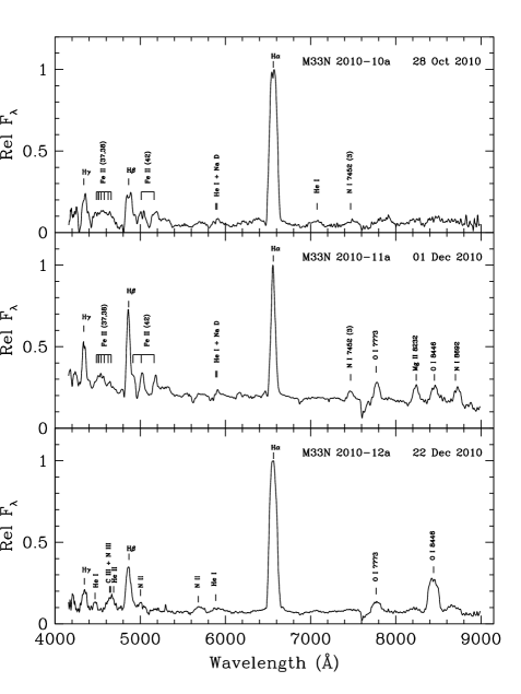
Figure 2: Spectra of the M33 novae M33N 1010-10a, 2010-11a, and 2010-12a, obtained two, four, and five days post-discovery, respectively. M33N 2010-10a and 2010-11a appear to be FeIIb (or Hybrid) novae with 2010-12a belonging to the He/N class.

We obtained a total of six spectra of M33 nova candidates, which are shown in Figures 1 and 2. Spectra were placed on relative flux scales through comparison with observations of spectrophotometric standards routinely used at the HET. Because the observations were made under a variety of atmospheric conditions with the stellar image typically overfilling the spectrograph slit, our data cannot be considered spectrophotometric. Thus, all spectra have been displayed on a relative flux scale. In the caption for each figure we have indicated the time elapsed between discovery of the nova (not necessarily maximum light) and the date of our spectroscopy.

2.2 Photometry

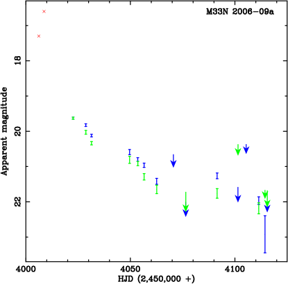
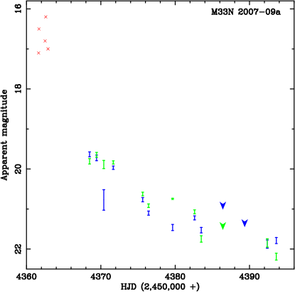
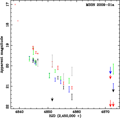
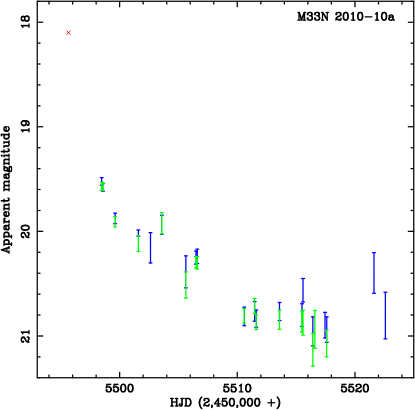
Figure 3: Light curves for M33N 2006-09a, M33N 2007-09a, M33N 2009-01a, and M33N 2010-10a. Uncertainties in measurements are shown as vertical bars with the following colors representing the different bandpasses: $B$ – blue; $V$ – green; $R$ – red. Upper flux limits are indicated by downward facing arrows.

To complement our spectroscopic survey, we were able to obtain photometry sufficient to produce light curves of four of the six novae in our spectroscopic survey. The data are given in Tables 2 and 3, with the light curves presented in Figure 3. Our primary motivation was to measure nova fade rates ($t_{2}$) that could then be correlated with other properties, such as spectroscopic class. The photometric data consist both of targeted (mostly $B$ and $V\/$-band) observations, which were obtained primarily with the Liverpool Telescope (LT, Steele et al., 2004) and the Faulkes Telescope North (FTN, Burgdorf et al., 2007). The LT and FTN data were reduced using a combination of IRAF and Starlink software, calibrated using standard stars from Landolt (1992), and checked against secondary standards from Magnier et al. (1992), Haiman et al. (1994), and Massey et al. (2006).

3 Spectroscopic Classification of Novae

The spectra of novae shortly after eruption (days to weeks) are characterized by an emission-line spectrum that is dominated by Balmer lines. In addition, novae also often display prominent emission lines of either Fe II (multiplet 42 is often the strongest) or He and N in various stages of ionization. The former group, referred to as the “Fe II” novae by Williams (1992) are often characterized by P Cygni-type line profiles, relatively narrow line widths (FWHM H$\alpha$ typically less than 2000 km s^-1), along with relatively slow spectral development over timescales of weeks. The latter class of novae, referred to as the “He/N” novae, display higher excitation emission lines that are generally broader (FWHM of H$\alpha$ $\mathrel{\hbox{\hbox to0.0pt{\hbox{\lower 4.0pt\hbox{$\sim$}}\hss}\hbox{$>$}}}$ 2500 km s^-1) with more rectangular, castellated or flat-topped profiles. It is remarkable that nova spectra can usually be classified into one of these two distinct groups, with Fe II novae making up $\sim$80% of Galactic and M31 novae (Shafter, 2007; Shafter et al., 2011b). A small fraction of novae appear to have characteristics of both classes. They are referred to as either “hybrid” or broad-lined Fe II (Fe IIb) novae. These novae appear similar to Fe II novae shortly after eruption, but the lines are broader than those seen in a typical Fe II nova. Later they may evolve to display a typical He/N spectrum. On the other hand He/N novae are never seen to evolve into Fe II novae. The classifications are robust, and with the exception of the hybrid novae, they are not particularly sensitive to the precise time during the first few weeks after eruption when the spectra are obtained.

Nova outbursts result from a thermonuclear runaway that occurs in the degenerate surface layers of a white dwarf that accretes matter from its companion. The resulting eruption ejects some or all of the accreted material, and in some cases may dredge up material from the white dwarf itself. Whether a particular nova becomes a Fe II, He/N or hybrid system ultimately must depend on the properties of the progenitor binary (principally the white dwarf mass and its accretion rate), which govern the physical conditions in the accreted layer at the time the nova is triggered. Numerical models of nova eruptions suggest that gas is ejected from the white dwarf in two distinct stages: a discrete shell of gas ejected at the time of eruption followed by steady mass loss in a wind (Williams, 1992). Radiation from the ejected gas then produces the emission-line spectrum that is typical of novae shortly after eruption. According to Williams (1992), the fundamental characteristics of the post-eruption nova spectrum, and thus the spectroscopic classification, depends on whether the dominant emission is produced in the discrete shell or in the wind. In an He/N nova it is thought that a relatively small amount of gas is ejected quickly, with little contribution from a wind, causing the spectrum to be dominated by emission from a high-velocity shell ionized by the hot white dwarf. In an Fe II nova, a larger accreted mass results in a more massive ejecta consisting of both a relatively low density, high velocity shell and an optically-thick wind driven by residual nuclear burning on the surface of the white dwarf.

Models of nova eruptions show that a TNR is triggered when the temperature and density at the base of the accreted envelope become sufficiently high for nuclear burning to take place (Starrfield et al., 2008). As shown by Townsley & Bildsten (2005) the amount of mass that must be accreted to trigger a TNR (the ignition mass) is primarily a function of the white dwarf mass and temperature, with the latter being strongly influenced by the rate of accretion onto the white dwarf’s surface. Thus, it seems plausible to expect that nova binaries with the most massive white dwarfs and with the highest accretion rates should have the smallest accreted masses and the shortest recurrence times between eruptions. Further, assuming the ejected mass is proportional to the accreted mass, such systems should be more likely to eject their mass in a discrete shell with little mass left over for residual burning on the white dwarf’s surface. They would then be expected to produce He/N spectra. On the other hand, nova progenitors harboring lower mass white dwarfs will have to accrete a greater envelope mass prior to TNR. It is these systems that are more likely to produce a higher mass of ejected material with a component in the form of an optically thick wind. Such systems are expected to be characterized by Fe II-type spectra.

4 Novae in M33

The first recorded M33 nova was discovered on a plate taken by F.G. Pease on the night of 1919 December 14 (Hubble, 1926). Discoveries continued only sporadically since then with a total of 36 novae and nova candidates reported in M33 up through the end of 2010 (e.g., Pietsch, 2010; Williams & Shafter, 2004; Della Valle et al., 1994; Sharov, 1993; Rosino & Bianchini, 1973, and references therein). The number of novae discovered in recent years has increased dramatically as a result of automated surveys and increased amateur astronomer activity, with almost half of the known M33 novae being discovered in the past 15 years. A summary of known M33 novae is presented in Table 4.

4.1 Spectroscopic Classifications

Given the transient nature of novae and the challenges of scheduling time on large telescopes with short notice, it is not surprising that the vast majority of M33 nova candidates have not been confirmed spectroscopically. The first known spectrum was reported less than a decade ago by Schwarz et al. (2003) who classified M33N 2003-09a as a member of the Fe II spectroscopic class. As part of a spectroscopic survey of novae in local group galaxies with the HET that began in 2006, we have obtained spectra of an additional six M33 novae over the past five years (see Figures 1 and 2). During this period, Di Mille et al. (2008) obtained a spectrum of 2008-02a and concluded that the system was a member of the Fe II class. Thus, there are a total of eight M33 novae for which a spectroscopic classification is currently possible. Following the classification scheme of Shafter et al. (2011b) for M31 novae, the six spectra included in our M33 survey were examined and subsequently assigned to one of four possible classes: Fe II, He/N, hybrid (also known as broad-lined Fe II or Fe IIb novae), and a potentially new class of narrow-lined He/N systems, the He/Nn novae. Below we summarize the properties of M33 novae with measured spectra.

$\bullet$ M33N 2003-09a: M33N 2003-09a was discovered at Lick Observatory by M. Ganeshalinam and W. Li with the Katzman Automated Imaging Telescope on Sep. 01.4 UT at $m=16.9$ (Ganeshalinam & Li, 2003). A little less than two days later on Sep. 03.05 Shporer etal. (2003) found the brightness of the nova relatively unchanged at $V=16.9$. A spectrum obtained approximately two weeks post-discovery by Schwarz et al. (2003) with the MMT revealed the object to be a likely member of the Fe II spectroscopic class. The rather large reported width of the H$\alpha$ line (FWZI $\sim 5400$ km s^-1) suggests that the nova may possibly be a member of the Fe IIb or hybrid class. No information is available concerning the speed class of this nova.

$\bullet$ M33N 2006-09a: M33N 2006-09a was discovered independently by R. Quimby et al. and by S. Nakano on Sep 28.20 UT ($m\sim 16.9$) and Sep. 30.68 UT ($m\sim 16.6$), respectively (Quimby et al., 2006; Itagaki, 2006). As part of our survey, a spectrum of 2006-09a was obtained on Oct. 02.42 with the HET (Shafter et al., 2006). The spectrum, shown in Figure 1, reveals the nova to be a typical member of the Fe II spectroscopic class. The light curve, shown in Figure 3, indicates that the nova faded moderately slowly with $t_{2}[B]\sim t_{2}[V]\sim 34$ days.

$\bullet$ M33N 2007-09a: M33N 2007-09a was discovered by K. Nishiyama and F. Kabashima on Sep. 18.63 UT at $m\sim 17.1$ (Nakano, 2007). A spectrum obtained approximately two days post-discovery by Wagner et al. (2007) revealed intense and broad Balmer and He I emission lines indicating that the nova was a member of the He/N class. Our HET spectrum, which was obtained approximately four days post-discovery on Sep. 22.25 UT (Shafter et al., 2007), confirms the He/N classification (see Figure 1). Subsequent photometry obtained with the LT revealed that the nova faded relatively rapidly (consistent with the He/N classification) with $t_{2}[B]\sim 11$ d and $t_{2}[V]\sim 6$ d (see Figure 3).

$\bullet$ M33N 2008-02a: K. Nishiyama and F. Kabashima discovered M33N 2008-02a on Feb. 27.47 UT at $m\sim 16.5$ (Nakano, 2008). Subsequently, a spectrum obtained on Mar. 2.80 UT revealed the nova to be a member of the Fe II class (Di Mille et al., 2008). No light curve information is available for this nova.

$\bullet$ M33N 2009-01a: M33N 2009-01a was discovered by K. Nishiyama and F. Kabashima, who found the nova to reach $m\sim 17.0$ on Jan 07.54 UT (Nakano, 2009). We obtained an HET spectrum of the nova approximately a week post-discovery on Jan. 14.14 UT (Shafter et al., 2009). The spectrum, shown in Figure 1, reveals H, He, and N emission lines with a complex structure consisting of both a broad base component with a narrower core component (see Table 5). The light curve obtained from our LT photometry and shown in Figure 3 reveals that the nova was moderately fast as expected for an He/N nova, being characterized by $t_{2}\sim 17$ days and $t_{2}\sim 12$ days for the $B$ and $V$ bandpasses, respectively.

$\bullet$ M33N 2010-10a: Like the previous 3 M33 novae, M33N 2010-10a was also discovered by K. Nishiyama and F. Kabashima who found the nova at $m\sim 18.1$ (unfiltered) on Oct. 26.654 UT (Yusa, 2010a). In order to classify the nova, we obtained an HET spectrum on Oct. 28.37 UT (see Figure 2), which revealed broad Balmer (FWHM H$\alpha$ $\sim 4200$ km s^-1), He, N, and Fe II emission lines (Shafter et al., 2010a). The presence of the Fe II emission suggests that this nova should be classified as a member of the Fe IIb, or hybrid spectroscopic class. Photometry obtained with the LT has enabled us to produce the light curve shown in Figure 3. The decline from maximum light was moderately fast with $t_{2}\sim 23$ d and $t_{2}\sim 20$ d, for the $B$ and $V$ bandpasses, respectively.

$\bullet$ M33N 2010-11a: M33N 2010-11a was discovered by J. Ruan and X. Gao on Nov. 27.53 UT at $m=18.6$ and independently by K. Nishiyama on Nov. 28.54 UT at $m=16.7$. The nova continued to brighten, reaching $m=16.1$ on Nov 29.064 UT (Yusa, 2010b). We obtained a spectrum of 2010-11a (see Figure 2) on Dec. 01.05 UT (Shafter et al., 2010b). The spectrum is characterized by relatively broad Balmer, He I, Fe II (and possibly N I) emission lines (FWHM H$\alpha$ $\sim 2600$ km s^-1), and can best be described as that of a broad-lined Fe II, or hybrid nova.

$\bullet$ M33N 2010-12a: M33N 2010-12a was discovered on Dec. 17.42 UT at $m=16.6$ (Yusa, 2010c). We obtained a spectrum (see Figure 2) of the nova 5 days later on Dec. 22.20 UT with the HET (Shafter et al., 2010c). The broad Balmer, He, and N emission (FWHM H$\alpha$ $\sim 4100$ km s^-1) clearly establish the nova as a member of the He/N spectroscopic class.

In summary, when all eight novae with observed spectra are considered (see Table 4), we find that five of the eight systems are either He/N or related systems (Fe IIb and hybrid), with Fe II novae making up less than 40% of the total. Despite the relatively small number of M33 novae that have been classified, this result appears to be in sharp contrast to the data for M31 and the Galaxy where Fe II novae comprise roughly 80% and 70% of the total, respectively (Shafter et al., 2011b). The somewhat higher percentage of Fe II novae observed in M31 relative to the Galaxy may reflect the fact that nova surveys have concentrated primarily on the bulge of M31, whereas Galactic data are biased to relatively nearby novae mostly located in the Galactic disk.

It is possible that as a result of outburst evolution our spectroscopic classifications may depend on the precise timing of the observations. For example, in hybrid novae, as the outburst progresses the spectrum evolves from a (broad-lined) Fe II spectrum to that resembling an He/N spectrum. On the other hand, novae have not been observed to evolve in the opposite sense, from He/N to Fe II class. Thus, if our classifications do evolve, it will likely result in fewer novae being classified as Fe II, and will exacerbate the discrepancy with the M31 and Galactic data.

4.1.1 Expansion Velocities

One of the defining properties of the He/N spectroscopic class is that the emission line widths are considerably broader than those seen in the Fe II novae. Specifically, Williams (1992) found that the emission lines of Galactic novae in the He/N class are typically characterized by a half-width at zero intensity, HWZI $>2500$ km s^-1. Empirically, we have found that for most nova line profiles the HWZI $\simeq$ FWHM; since the latter is the more easily measured quantity, we have followed Shafter et al. (2011b) and adopted the FWHM to characterize the spectra in our survey. The values of the FWHM and the equivalent widths of H$\alpha$ and H$\beta$ in our nova spectra are given in Table 5. Without exception, as in M31 (Shafter et al., 2011b), the novae belonging to the He/N class are characterized by H$\alpha$ FWHM $>2500$ km s^-1, while the Fe II systems all have an FWHM less than this value.

Although the emission line width is expected to be correlated with the expansion velocity of the nova ejecta, the FWHM does not necessarily yield the expansion velocity directly. In an Fe II nova, the lines are mainly produced in a wind, which originates at a distance above the surface of the white dwarf that varies as the outburst evolves. Thus, the escape velocity for this wind is smaller than that at the white dwarf’s surface. As a result, the derived expansion velocity (and hence line width) may decrease with the time elapsed since eruption. In an He/N nova, on the other hand, the broad emission features are believed to be formed mainly in a discrete, optically-thin shell ejected at relatively high velocity from near the white dwarf’s surface. The line profiles are expected to be flat-topped with the FWHM closely approximating the ejection velocity of the shell.

4.2 Light Curve Properties

To further explore the properties of the novae in our survey, whenever possible we have augmented our spectroscopic data with available photometric observations. Unfortunately, we could find no light curve information for M33 novae erupting prior to the start of our HET spectroscopic survey in 2006. Nevertheless, we have sufficient photometric data to estimate decline rates for half of the novae (four of eight) in our spectroscopic sample.

A convenient and widely used parameterization of the decline rate is $t_{2}$, which represents the time (in days) for a nova to decline 2 mag from maximum light. According to the criteria of Warner (2008), novae with $t_{2}\mathrel{\hbox{\hbox to0.0pt{\hbox{\lower 4.0pt\hbox{$\sim$}}\hss}\hbox{$<$}}}25$ days are considered “fast” or “very fast”, with the slowest novae characterized by $t_{2}$ values of several months or longer. Rates of decline, and corresponding values of $t_{2}$, have been measured for the 4 novae in our photometric sample by performing weighted linear least-squares fits to the declining portion of the light curves that extend up to 3 mag below peak. In an attempt to account for systematic errors in the individual photometric measurements, the weights used in the fits were composed of the sum of the formal errors on the individual photometric measurements plus a constant systematic error estimate of 0.1 mag. The net effect of including the systematic error component was a reduction of the relative weighting of points with small formal errors and a corresponding increase in the formal errors of the best-fit parameters and in the uncertainties in $t_{2}$ derived from them.

Because our photometric observations do not always begin immediately after discovery, and the date of discovery does not always represent the date of eruption, we have made two modifications to our photometric data in order to better estimate the light curve parameters. First, when available, we have augmented our light curve data with the discovery dates and magnitudes given in the catalog of Pietsch (2010). Secondly, for some novae we have modified (brightened) the peak magnitude slightly through an extrapolation of the declining portion of the light curve by up to 2.5 days pre-discovery in cases where upper flux limits (within five days of discovery) are available. Finally, apparent magnitudes at the time of discovery have been converted to estimates of the absolute magnitude at maximum light by adopting distance moduli for M33 of $\mu_{B}=25.35$ and $\mu_{V}=25.26$ (Pellerin & Macri, 2011). The light curve parameters resulting from our analysis are given in Table 6. In agreement with the results of both the Galactic study by Della Valle & Livio (1998) and the M31 study by Shafter et al. (2011b), it appears that the He/N novae in M33 are generally “faster” than their Fe II counterparts, as expected for novae with more massive white dwarfs (e.g., Livio, 1992).

4.3 The Spatial Distribution of M33 Novae

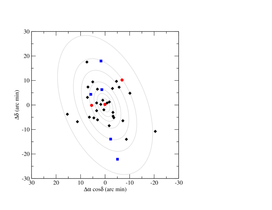
Figure 4: Spatial distribution of the 36 recorded novae in M33. The Fe II novae are indicated by filled red circles, while the He/N and Fe IIb (hybrid) novae are represented by filled blue squares. The black diamonds represent the 28 novae with unknown spectroscopic types. The gray ellipses represent elliptical isophotes from the surface photometry of Regan & Vogel (1994).

The projected positions of the 36 known M33 novae from Table 4 are shown in Figure 4. For the 8 novae with known spectroscopic class we have plotted the Fe II systems as filled circles and the He/N and Hybrid novae as filled squares. Observations by Della Valle & Livio (1998) suggest that Fe II and He/N novae are associated with different stellar populations: the He/N novae primarily with the Galactic disk and the Fe II novae with thick disk and bulge. Given that M33 is a nearly bulgeless galaxy, classified as an Scd galaxy (Tully & Fisher, 1988), the spatial distributions of the Fe II and He/N novae are not expected to differ significantly.

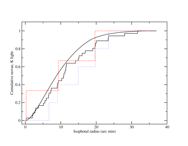
Figure 5: Cumulative distribution of the M33 novae compared with background K light from Regan & Vogel (1994). A K-S test indicates a 39% probability that the distributions would differ by more than they do under the null hypothesis that the distributions are drawn from the same parent population. For comparison, the Fe II systems (red dashed line) are compared with the He/N (Fe IIb) systems (blue dotted line).

M33 is oriented at an angle of $57^{\circ}$ with respect to the plane of the sky. Thus, in order to approximate the true position of a nova within M33, we have assigned each nova an isophotal radius, defined as the length of the semi-major axis of an elliptical isophote computed from the $R$-band surface photometry of Kent (1987) that passes through the observed position of the nova. In Figure 5, we show the cumulative distribution the M33 novae compared with the cumulative $K$-band light from the surface photometry of Regan & Vogel (1994). A Kolmogorov-Smirnov (K-S) test reveals that the distributions would be expected to differ by more than that observed 39% of the time if they were drawn from the same parent population. Thus, there is no reason to reject the hypothesis that the novae follow the light distribution in M33. We have also shown the cumulative distributions of the Fe II and He/N (and hybrid) novae separately, although we have insufficient data to draw any conclusions regarding whether these distributions may differ.

5 Discussion and Conclusions

The answer to the question of whether or not there exist two distinct populations of novae has remained elusive, with observational support for both sides of the issue. For example, an analysis of spectroscopic observations of Galactic novae by Della Valle & Livio (1998) suggests that He/N novae are generally located closer to the Galactic plane than are the Fe II novae, suggesting that the He/N novae belong to a younger stellar population compared with the latter class of novae. On the other hand, the recent spectroscopic survey of novae in M31 by Shafter et al. (2011b) finds no significant difference in the spatial distributions of the He/N and Fe II novae in that galaxy.

In an attempt to gain further insight into the question of whether the spectroscopic class of novae is sensitive to stellar population, we have initiated a spectroscopic survey of novae in the late-type, nearly bulgeless spiral galaxy, M33. Despite the fact that the absolute nova rate in M33 is only $\sim 2.5$ per year (Williams & Shafter, 2004), we were able to secure spectra for six novae thus far since our survey began in 2006. After including spectroscopic observations of two additional novae from the literature, we were ultimately able to establish spectroscopic classes for a total of eight novae in M33. Of the eight, only two novae (M33N 2006-09a and 2008-02a) are clearly members of the Fe II class, with a third nova, 2003-09a, possibly being a member of the Fe IIb class. Of the remaining novae, three are clearly He/N novae, with two being Fe IIb or hybrid objects.

Although the number of spectra available for M33 is currently small relative to M31, it is already clear that the fraction of Fe II novae in M33 is surprisingly low. We can estimate the significance of this result as follows. Let $p({\rm Fe~{}II})$ be the fraction of novae occurring within a galaxy with the spectroscopic classification Fe II, and let $q({\rm He/N})=1-p({\rm Fe~{}II})$ be the fraction of novae with spectroscopic classification He/N (+ Fe IIb). The probability of observing $N$ Fe II novae out of a sample of $M$ objects is simply

$$P_{N,M}={M!\over N!(M-N)!}\ p({\rm Fe~{}II})^{N}\,q({\rm He/N})^{M-N},$$ (1)

and the probability of observing $N$ or fewer Fe II novae is

$$P_{\leq N,M}=\sum_{n=0}^{N}P_{n,M}.$$ (2)

Under the null hypothesis that the novae in M33 have the same ratio of spectroscopic types as that seen in M31, we have $p({\rm Fe~{}II})=0.8$ and $q({\rm He/N})=0.2$, and the probability of observing three or fewer Fe II novae is $P_{\leq 3,8}=0.0104$. In other words, the mix of spectroscopic nova types in M33 differs from that of M31 at the 99% confidence level.

This result is perhaps not surprising given that the spectroscopic class of novae is expected to depend on fundamental physical properties of the nova progenitor binary such as the mass of the white dwarf. The average mass of the white dwarfs in nova binaries, in turn, is thought to be sensitive to the age of the underlying stellar population in the sense that a younger stellar population, like that which dominates in M33, should contain, on average, higher mass white dwarfs (e.g., de Kool, 1992; Tutukov & Yungelson, 1995; Politano, 1996). It therefore appears plausible that the observed difference in the mix of nova types in M31 and M33 might be related to the difference in stellar population between the two galaxies.

In addition to obtaining spectroscopic observations of M33 novae, we were able to measure light curves (and resulting $t_{2}$ times) for the majority of the novae in our sample, and for half of the novae with known spectroscopic class. Although our small sample does not allow us to study the spatial distribution of speed class as we were able to do in the case of M31 (Shafter et al., 2011b), we did find, as expected, that of the four novae with measured $t_{2}$, the fastest declining systems (M33N 2007-09a and 2009-01a) were members of the He/N spectroscopic class, while the slowest nova, 2006-09a, was found to be a member of the Fe II class.

Finally, by considering the positions of all 36 novae seen to erupt in M33 over the past century (Pietsch, 2010), we were able to explore the spatial distribution of novae across the galaxy. Although the available dataset is too limited to study the distributions of the Fe II and He/N novae separately, we did find that the overall nova distribution is consistent with that expected if the nova rate is proportional to the surface brightness distribution in the galaxy.

In order to confirm our preliminary findings, future observational efforts should focus not only on continued optical imaging to discover additional M33 nova candidates, but also on the timely spectroscopic and photometric follow-up observations required to increase the number of available spectroscopic and speed classifications. In addition, X-ray observations to measure the timing and duration of the nova supersoft stage can be used provide useful constraints on the properties of nova binaries in M33, as they have in studies of novae in M31 (e.g. Pietsch et al., 2007; Bode et al., 2009; Henze et al., 2010; Pietsch et al., 2011; Henze et al., 2011).

Figure 1: Spectra of the M33 novae M33N 2006-09a, 2007-09a, and 2009-01a taken four, four, and seven days post-discovery, respectively. M33N 2006-09a appears to be an Fe II system, while 2007-09a and 2009-01a are clearly He/N systems.

Table 1: Summary of HET Spectroscopic Observations

	R.A.	Decl.		Exp.	Coverage
Nova	(2000.0)	(2000.0)	UT Date	(sec)	(Å)	Weather
M33N 2006-09a	01 33 18.7	30 49 49	02 Oct 2006	1200	4300–7300	spec
M33N 2007-09a	01 33 58.6	30 57 34	22 Sep 2007	1200	4300–7300	spec
M33N 2009-01a	01 33 40.4	30 25 42	14 Jan 2009	1200	4300–7300	phot
M33N 2010-10a	01 33 57.1	30 45 53	28 Oct 2010	1300	4150–9000	phot
M33N 2010-11a	01 33 47.5	30 17 28	01 Dec 2010	1000	4150–9000	spec
M33N 2010-12a	01 34 18.0	30 43 58	22 Dec 2010	1200	4150–9000	spec

Table 2: Photometric Observations

$\mathrm{MJD}$
($50,000+$)	Filter	Mag
M33N 2006-09a
4022.119	$B$	$19.626\pm 0.028$
4028.185	$B$	$19.825\pm 0.037$
4030.918	$B$	$20.122\pm 0.036$
4049.125	$B$	$20.591\pm 0.073$
4053.045	$B$	$20.799\pm 0.051$
4056.056	$B$	$20.964\pm 0.061$
4062.083	$B$	$21.420\pm 0.083$
4070.081	$B$	$>20.663\pm 0.368$
4075.991	$B$	$>22.011\pm 0.417$
4090.996	$B$	$21.265\pm 0.081$
4100.974	$B$	$>21.591\pm 0.427$
4104.896	$B$	$>20.375\pm 0.268$
4110.916	$B$	$21.967\pm 0.108$
4113.898	$B$	$22.923\pm 0.526$
4114.964	$B$	$>22.110\pm 0.189$
4022.122	$V$	$19.629\pm 0.029$
4028.188	$V$	$20.029\pm 0.053$
4030.921	$V$	$20.339\pm 0.046$
4049.128	$V$	$20.810\pm 0.101$
4053.049	$V$	$20.914\pm 0.061$
4056.059	$V$	$21.292\pm 0.091$
4062.086	$V$	$21.650\pm 0.119$
4075.995	$V$	$>21.729\pm 0.560$
4090.999	$V$	$21.763\pm 0.134$
4100.978	$V$	$>20.377\pm 0.315$
4110.919	$V$	$22.185\pm 0.156$
4113.901	$V$	$>21.675\pm 0.242$
4114.967	$V$	$>21.688\pm 0.469$
M33N 2007-09a
4368.986	$B$	$19.807\pm 0.066$
4369.931	$B$	$19.647\pm 0.061$
4370.896	$B$	$19.889\pm 0.102$
4372.176	$B$	$19.835\pm 0.039$
4376.130	$B$	$20.625\pm 0.046$
4376.919	$B$	$20.917\pm 0.045$
4380.152	$B$	$20.745\pm 0.015$
4383.104	$B$	$21.070\pm 0.048$
4384.000	$B$	$21.748\pm 0.080$
4386.909	$B$	$>21.443\pm 0.078$
4392.885	$B$	$21.847\pm 0.104$
4394.099	$B$	$22.189\pm 0.086$
4368.989	$V$	$19.633\pm 0.061$
4369.934	$V$	$19.723\pm 0.070$
4370.899	$V$	$20.773\pm 0.255$
4372.179	$V$	$19.967\pm 0.042$
4376.132	$V$	$20.768\pm 0.052$
4376.921	$V$	$21.103\pm 0.051$
4380.154	$V$	$21.462\pm 0.077$
4383.107	$V$	$21.221\pm 0.051$
4384.003	$V$	$21.528\pm 0.069$
4386.911	$V$	$>20.951\pm 0.061$
4389.848	$V$	$>21.372\pm 0.078$
4392.888	$V$	$21.877\pm 0.102$
4394.102	$V$	$21.787\pm 0.076$
M33N 2009-01a
4843.999	$B$	$19.663\pm 0.106$
4845.944	$B$	$19.773\pm 0.054$
4850.981	$B$	$20.476\pm 0.120$
4852.971	$B$	$20.255\pm 0.069$
4854.932	$B$	$20.602\pm 0.073$
4857.860	$B$	$20.733\pm 0.124$
4844.266	$B$	$19.713\pm 0.030$
4844.374	$B$	$19.719\pm 0.059$
4845.304	$B$	$19.891\pm 0.038$
4871.271	$B$	$>20.056\pm 0.349$
4872.299	$B$	$>21.055\pm 0.184$
4844.001	$V$	$19.608\pm 0.070$
4845.948	$V$	$19.846\pm 0.057$
4850.984	$V$	$20.481\pm 0.103$
4852.982	$V$	$20.679\pm 0.085$
4854.944	$V$	$20.791\pm 0.085$
4857.862	$V$	$21.153\pm 0.139$
4844.271	$V$	$19.645\pm 0.032$
4844.379	$V$	$19.283\pm 0.165$
4845.309	$V$	$19.879\pm 0.097$
4872.301	$V$	$>20.160\pm 0.247$
4845.934	$r^{\prime}$	$19.401\pm 0.019$
4850.969	$r^{\prime}$	$19.920\pm 0.129$
4852.951	$r^{\prime}$	$20.100\pm 0.088$
4854.912	$r^{\prime}$	$20.851\pm 0.065$
4857.840	$r^{\prime}$	$21.074\pm 0.066$
4844.251	$r^{\prime}$	$19.152\pm 0.017$
4844.283	$r^{\prime}$	$19.060\pm 0.019$
4844.359	$r^{\prime}$	$19.180\pm 0.038$
4845.289	$r^{\prime}$	$19.350\pm 0.055$
4871.256	$r^{\prime}$	$>20.455\pm 0.202$
4871.274	$r^{\prime}$	$>21.679\pm 0.340$
4872.270	$r^{\prime}$	$>21.772\pm 0.238$
4845.938	$i^{\prime}$	$19.695\pm 0.027$
4850.973	$i^{\prime}$	$>21.556\pm 0.186$
4852.955	$i^{\prime}$	$20.584\pm 0.071$
4854.916	$i^{\prime}$	$21.063\pm 0.075$
4857.843	$i^{\prime}$	$21.523\pm 0.143$
4844.256	$i^{\prime}$	$19.795\pm 0.047$
4844.364	$i^{\prime}$	$19.700\pm 0.043$
4845.294	$i^{\prime}$	$19.802\pm 0.049$
4872.275	$i^{\prime}$	$>21.158\pm 0.137$
4845.943	$z^{\prime}$	$19.900\pm 0.126$
4850.977	$z^{\prime}$	$19.774\pm 0.308$
4854.920	$z^{\prime}$	$20.546\pm 0.159$
4857.848	$z^{\prime}$	$20.275\pm 0.210$
M33N 2010-10a
5499.084	$B$	$19.574\pm 0.035$
5498.972	$B$	$19.570\pm 0.038$
5500.112	$B$	$19.908\pm 0.049$
5502.088	$B$	$20.117\pm 0.076$
5504.087	$B$	$19.922\pm 0.101$
5506.126	$B$	$20.513\pm 0.125$
5507.093	$B$	$20.300\pm 0.060$
5506.984	$B$	$20.296\pm 0.054$
5511.085	$B$	$20.808\pm 0.068$
5511.965	$B$	$20.714\pm 0.072$
5512.106	$B$	$20.868\pm 0.070$
5514.087	$B$	$20.844\pm 0.092$
5516.084	$B$	$20.873\pm 0.119$
5515.990	$B$	$20.862\pm 0.101$
5517.094	$B$	$20.937\pm 0.181$
5516.918	$B$	$21.133\pm 0.156$
5518.095	$B$	$21.073\pm 0.127$
5499.087	$V$	$19.580\pm 0.036$
5498.975	$V$	$19.522\pm 0.036$
5500.115	$V$	$19.876\pm 0.050$
5502.091	$V$	$20.017\pm 0.030$
5503.121	$V$	$20.157\pm 0.145$
5504.090	$V$	$19.937\pm 0.091$
5506.129	$V$	$20.387\pm 0.153$
5507.095	$V$	$20.238\pm 0.069$
5506.986	$V$	$20.250\pm 0.063$
5511.088	$V$	$20.813\pm 0.089$
5511.968	$V$	$20.765\pm 0.094$
5512.109	$V$	$20.834\pm 0.082$
5514.090	$V$	$20.766\pm 0.086$
5516.087	$V$	$20.563\pm 0.112$
5515.993	$V$	$20.801\pm 0.109$
5516.921	$V$	$20.956\pm 0.139$
5518.097	$V$	$20.939\pm 0.122$
5517.955	$V$	$20.897\pm 0.123$
5522.114	$V$	$20.397\pm 0.194$
5523.086	$V$	$20.805\pm 0.223$

Table 3: Supplemental Photometry

$\mathrm{MJD}$
($50,000+$)	Filter	Mag	References
M33N 2006-09a
4006.200	$W$	$17.3$	1
4008.684	$W$	$17.6$	2
M33N 2007-09a
4361.630	$W$	$17.1$	3
4361.677	$W$	$16.5$	3
4362.501	$R$	$16.2$	3
4362.503	$W$	$16.8$	3
4362.896	$W$	$17.0$	4
M33N 2009-01a
4838.536	$W$	$17.0$	5
4839.475	$W$	$17.8$	5
M33N 2010-10a
5495.654	$W$	$18.1$	6

Table 4: M33 Novae

	JD	$\Delta\alpha~{}cos\delta$	$\Delta\delta$	$a$	Discovery
Nova	Discovery	(′)	(′)	(′)	mag (Filter)	Type	References
M33N 1919-12a	2422306.5	1.75	0.24	2.86	17.2 (pg)	…	1
M33N 1922-08a	2423292.	-4.65	9.66	16.02	17.5 (pg)	…	1
M33N 1925-07a	2424348.5	5.04	9.44	10.79	17.9 (pg)	…	1
M33N 1925-12a	2424493.3	4.59	-5.26	11.62	18.1 (pg)	…	1
M33N 1927-07a	2425091.6	-5.73	7.26	15.15	17.7 (pg)	…	1
M33N 1927-09a	2425124.5	0.50	-1.96	2.71	…	…	1
M33N 1928-10a	2425534.5	-1.68	-8.45	9.00	16.0 (pg)	…	1
M33N 1949-08a	2433157.5	-20.48	-10.77	31.69	16.6 (pg)	…	1
M33N 1955-07a	2435289.5	-3.54	-5.18	6.54	17.2 (V)	…	1
M33N 1960-11a	2437253.51	3.46	0.84	5.52	16.4 (pg)	…	1
M33N 1961-03a	2437365.32	15.38	-3.77	28.03	18.5 (pg)	…	1
M33N 1961-11a	2437632.29	3.08	-6.06	10.27	18.0 (pg)	…	1
M33N 1962-09a	2437917.56	-10.13	4.81	20.01	18.0 (pg)	…	1
M33N 1962-09b	2437929.53	0.94	1.94	2.16	17.3 (pg)	…	1
M33N 1969-11a	2440529.78	6.98	7.33	11.41	18.0 (V)	…	1
M33N 1970-09a	2440836.	7.42	17.53	19.04	18.0 (pg)	…	1
M33N 1974-12a	2442386.5	11.28	-6.81	23.37	16.3 (pg)	…	1
M33N 1975-10a	2442691.5	-3.21	-3.02	5.12	18.8 (pg)	…	1
M33N 1977-12a	2443506.5	-8.69	-14.01	16.90	17.9 (pg)	…	1
M33N 1982-09a	2445229.41	3.13	6.46	7.20	17.9 (B)	…	1
M33N 1986-10a	2446703.36	-3.27	-4.56	5.90	18.5 (B)	…	1
M33N 1995-08a	2449955.5	-0.82	0.82	1.96	16.0 (Ha)	…	1
M33N 1995-08b	2449957.5	-7.26	-6.43	11.49	16.6 (Ha)	…	1
M33N 1995-09a	2450012.5	3.44	-2.32	7.32	16.2 (Ha)	…	1
M33N 1996-12a	2450426.5	6.41	-4.96	14.16	19.1 (Ha)	…	1
M33N 1997-09a	2450692.5	7.20	3.10	11.21	19.3 (Ha)	…	1
M33N 2001-11a	2452229.26	-1.74	1.25	3.76	16.5 (w)	…	1
M33N 2003-09a	2452883.9	0.06	0.22	0.23	16.9 (w)	Fe IIb?	2
M33N 2006-09a	2454006.7	-6.92	10.21	19.67	16.6 (w)	Fe II	3
M33N 2007-09a	2454362.13	1.66	17.96	19.78	16.2 (R)	He/N	3,4
M33N 2008-02a	2454523.97	5.49	-0.14	9.34	16.5 (w)	Fe II	5
M33N 2009-01a	2454839.04	-2.26	-13.91	14.95	17.0 (w)	He/N	3
M33N 2010-07a	2455376.5	-3.02	6.75	10.90	17.1 (w)	…	1
M33N 2010-10a	2455496.15	1.33	6.27	6.66	17.7 (w)	Fe IIb	3
M33N 2010-11a	2455528.03	-5.04	-22.14	23.47	16.1 (w)	Fe IIb	3
M33N 2010-12a	2455547.92	5.82	4.36	9.06	16.4 (w)	He/N	3

Table 5: Balmer Emission Line Properties

	EW (Å)		FWHM (km s-1)
Nova	H$\beta$	H$\alpha$	H$\beta$	H$\alpha$	Type	References
M33N 2003-09a	…	…	…	2700:	Fe IIb?	1
M33N 2006-09a	$-85$	$-190$	1420	1370	Fe II	2
M33N 2007-09a	$-160$	$-760$	4260	4800	He/N	2
M33N 2008-02a	…	…	…	1700	Fe II	3
M33N 2009-01a (narrow)	…	…	1670	2510	He/N	2
M33N 2009-01a (broad)	…	…	7220	5970	He/N	2
M33N 2010-10a	$-270$	$-1630$	5060	4210	Fe IIb	2
M33N 2010-11a	$-110$	$-220$	2800	2610	Fe IIb	2
M33N 2010-12a	$-170$	$-1020$	3860	4070	He/N	2

Table 6: Light Curve Parameters

Nova	Filter	$M_{max}$	Fade Rate (mag d-1)	$t_{2}$ (days)
M33N 2006-09a	$B$	$-8.12\pm 0.15$	$0.059\pm 0.003$	$33.7\pm 1.7$
	$V$	$-8.46\pm 0.15$	$0.059\pm 0.003$	$33.8\pm 1.8$
M33N 2007-09a	$B$	$-8.53\pm 0.15$	$0.183\pm 0.006$	$11.0\pm 0.3$
	$V$	$-8.93\pm 0.15$	$0.342\pm 0.013$	$5.9\pm 0.2$
M33N 2009-01a	$B$	$-7.65\pm 0.15$	$0.120\pm 0.007$	$16.7\pm 1.0$
	$V$	$-7.99\pm 0.15$	$0.168\pm 0.008$	$11.9\pm 0.5$
M33N 2010-10a	$B$	$-6.55\pm 0.15$	$0.086\pm 0.005$	$23.1\pm 1.3$
	$V$	$-6.89\pm 0.15$	$0.098\pm 0.006$	$20.4\pm 1.2$

References

- Burgdorf et al. (2007) Burgdorf, M. J., Bramich, D. M., Dominik, M., Bode, M. F., Horne, K. D., Steele, I. A., Rattenbury, N., & Tsapras, Y. 2007, P&SS, 55, 582
- Bode et al. (2009) Bode, M. F., Darnley, M. J., Shafter, A. W., Page, K. L., Smirnova, O., Anupama, G. C., Hilton, T. 2009, ApJ, 705, 1056
- Ciardullo et al. (1987) Ciardullo, R., Ford, H. C., Neill, J. D., Jacoby, G. H., & Shafter, A. W. 1987, ApJ, 318, 520
- de Kool (1992) de Kool, M. 1992, A&A, 261, 188
- Darnley et al. (2006) Darnley et al. 2006, MNRAS, 365, 1099
- Della Valle et al. (1992) Della Valle, M., Bianchini, A., Livio, M., & Orio, M. 1992, A&A, 266, 232
- Della Valle et al. (1994) Della Valle, M., Rosino, L., Bianchini, A., & Livio, M. 1994, ApJ, 287, 403
- Della Valle & Livio (1998) Della Valle, M., & Livio, M. 1998, ApJ, 506, 818
- Di Mille et al. (2008) di Mille, F., Ciroi, S., Cracco, V., Rafanelli, P., Temporin, S. 2008, CBET 1284
- Duerbeck (1990) Duerbeck, H. W. 1990, in Physics of Classical Novae, ed. A.Cassatella & R. Viotti, (New York: Springer-Verlag), 96
- Ferrarese et al. (2003) Ferrarese, L., Côté, P., Jordán, A. 2003, ApJ, 599, 1302
- Ganeshalinam & Li (2003) Ganeshalinam, M. & Li, W. 2003, IAU Circ. 8195
- Haiman et al. (1994) Haiman et al., 1994, A&A, 286, 725
- Henze et al. (2010) Henze, M. et al. 2010, A&A, 523, 89
- Henze et al. (2011) Henze, M. et al. 2011, A&A, 533, 52
- Hill et al. (1998) Hill, G. J., Nicklas, H. E., MacQueen, P. J., Tejada, C., Cobos Duenas, F. J., & Mitsch, W. 1998, Proc. SPIE, 3355, 375
- Hounsell et al. (2010) Hounsell et al. 2010, ApJ, 724, 480
- Hornoch et al. (2008) Hornoch, K., Scheirich, P., Garnavich, P. M., Hameed, S. & Thilker, D. A. 2008, A&A, 492, 301
- Hubble (1926) Hubble, E. P. 1926, ApJ, 63, 236
- Itagaki (2006) Itagaki, K. 2006, CBET 655
- Kent (1987) Kent, S. M. 1987, AJ, 94, 306
- Kugel (2007) Kugel, F. 2007, CBET 1080
- Landolt (1992) Landolt, 1992, AJ, 104, 340
- Livio (1992) Livio, M. 1992, ApJ, 393, 516
- Magnier et al. (1992) Magnier et al.,1992, A&AS, 96, 379
- Massey et al. (2006) Massey et al., 2006, AJ, 131, 2478
- Nakano (2007) Nakano, S. 2007, CBET 1074
- Nakano (2008) Nakano, S. 2008, CBET 1272
- Nakano (2009) Nakano, S. 2009, CBET 1659
- Pellerin & Macri (2011) Pellerin, A & Macri, L. M. 2011, ApJS, 193, 26
- Pietsch et al. (2007) Pietsch, W., Haberl, F., Sala, G., Stiele, H., Hornoch, K., Riffeser, A., Fliri, J., Bender, R., Bühler, S., Burwitz, V., Greiner, J. & Seitz, S. 2007, A&A, 465, 375
- Pietsch (2010) Pietsch, W. 2007, Astronomische Nachrichten, 331, 187
- Pietsch et al. (2011) Pietsch, W., Henze, M., Haberl, F., Hernanz, M., Sala, G., Hartmann, D. H., Della Valle, M. 2011, A&A, 531, 22
- Politano (1996) Politano, M. 1996, ApJ, 465, 338
- Quimby et al. (2006) Quimby, R., Mondol, P., & Castro, F. 2006, CBET 655
- Rosino & Bianchini (1973) Rosino, L. & Bianchini, A. 1973, A&A, 22, 461
- Regan & Vogel (1994) Regan, M. W. & Vogel, S. N. 1994, ApJ, 434, 536
- Schwarz et al. (2003) Schwarz, G. J., Wagner, R. M, Starrfield, S., Szkody, P. 2003, IAUC 8234
- Shafter (1997) Shafter, A. W. 1997, ApJ, 487, 226
- Shafter et al. (2000) Shafter, A. W., Ciardullo, R., & Pritchet, C. J. 2000, ApJ, 530, 193
- Shafter & Irby (2001) Shafter, A. W. & Irby, B. K. 2001, ApJ, 563, 749
- Shafter (2002) Shafter, A. W. 2002, in Classical Nova Explosions, edited by M. Hernanz, and J. José, AIP Conference Proceedings 637, p. 462
- Shafter et al. (2006) Shafter, A. W., Coelho, E. A., Misselt, K. A., Bode, M. F., Darnley, M. J., Quimby, R. 2006, ATel 923
- Shafter (2007) Shafter, A. W. 2007, BAAS, 211.5115
- Shafter et al. (2007) Shafter, A. W., Bode, M. F., Darnley, M. J., Misselt, K. A., Quimby, R.; Yuan, F. 2007, ATel 1225
- Shafter (2008) Shafter, A. W. 2008, in Classical Novae, 2nd ed., edited by M. Bode and A. Evans, Cambridge University press, p. 335
- Shafter et al. (2009) Shafter, A. W., Ciardullo, R., Bode, M. F., Darnley, M. J., Misselt, K. A. 2009b, ATel 1900
- Shafter et al. (2010a) Shafter, A. W., Ciardullo, R., Bode, M. F., Darnley, M. J., Misselt, K. A. 2010a, ATel 2982
- Shafter et al. (2010b) Shafter, A. W., Ciardullo, R., Bode, M. F., Darnley, M. J., Misselt, K. A. 2010b, ATel 3063
- Shafter et al. (2010c) Shafter, A. W., Ciardullo, R., Bode, M. F., Darnley, M. J., Misselt, K. A. 2010c, ATel 3086
- Shafter et al. (2011a) Shafter, A. W., Bode, M. F., Darnley, M. J., Misselt, K. A., Rubin, M., Hornoch, K. 2011a, ApJ, 727, 50
- Shafter et al. (2011b) Shafter, A. W., Darnley, M. J., Hornoch, K., Filippenko, A. V., Bode, M. F., Ciardullo, R., Misselt, K. A., Hounsell, R. A., Chornock, R., Matheson, T. 2011b, ApJ, 734, 12
- Sharov (1993) Sharov, A. S. 1993, Astron. Lett., 19, 3
- Shporer etal. (2003) Shporer, A., Ofek, E. O., & Mazeh, T. 2003, IAU Circ. 8199
- Starrfield et al. (2008) Starrfield, S., Iliadis, C., & Hix, R. 2008, in Classical Novae, 2nd ed., edited by M. Bode and A. Evans, Cambridge University Press, p. 77
- Steele et al. (2004) Steele I. A., et al., 2004, SPIE, 5489, 679
- Townsley & Bildsten (2005) Townsley, D. M., Bildsten, L. 2005, ApJ, 628, 395
- Tully & Fisher (1988) Tully, R. B. & Fisher, R. J. 1988, Catalog of Nearby Galaxies, Cambridge University Press.
- Tutukov & Yungelson (1995) Tutukov, A. V. & Yungelson, L. R. 1995, Cataclysmic Variables, Proceedings of the conference held in Abano Terme, Italy, 20-24 June 1994 Publisher: Dordrecht Kluwer Academic Publisher:s, 1995. Edited by A. Bianchini, M. della Valle, and M. Orio. Astrophysics and Space Science Library, Vol. 205, p.495
- Wagner et al. (2007) Wagner, R. M, Starrfield, S., Schwarz, G. 2007, CBET 1080
- Warner (1995) Warner, B. 1995, in Cataclysmic Variable Stars, Cambridge University Press.
- Warner (2008) Warner, B. 2008, in Classical Novae, 2nd ed., edited by M. Bode and A. Evans, Cambridge University Press, p. 16
- Williams (1992) Williams, R. E. 1992, AJ, 104, 725
- Williams & Shafter (2004) Williams, S. J. & Shafter, A. W. 2004, ApJ, 612, 867
- Yusa (2010a) Yusa, T. 2010a, CBET 2533
- Yusa (2010b) Yusa, T. 2010b, CBET 2559
- Yusa (2010c) Yusa, T. 2010c, CBET 2595