Numerical Approaches for Multidimensional Simulations of Stellar Explosions

Abstract

We introduce numerical algorithms for initializing multidimensional simulations of stellar explosions with 1D stellar evolution models. The initial mapping from 1D profiles onto multidimensional grids can generate severe numerical artifacts, one of the most severe of which is the violation of conservation laws for physical quantities. We introduce a numerical scheme for mapping 1D spherically-symmetric data onto multidimensional meshes so that these physical quantities are conserved. We verify our scheme by porting a realistic 1D Lagrangian stellar profile to the new multidimensional Eulerian hydro code CASTRO. Our results show that all important features in the profiles are reproduced on the new grid and that conservation laws are enforced at all resolutions after mapping. We also introduce a numerical scheme for initializing multidimensional supernova simulations with realistic perturbations predicted by 1D stellar evolution models. Instead of seeding 3D stellar profiles with random perturbations, we imprint them with velocity perturbations that reproduce the Kolmogorov energy spectrum expected for highly turbulent convective regions in stars. Our models return Kolmogorov energy spectra and vortex structures like those in turbulent flows before the modes become nonlinear. Finally, we describe approaches to determining the resolution for simulations required to capture fluid instabilities and nuclear burning. Our algorithms are applicable to multidimensional simulations besides stellar explosions that range from astrophysics to cosmology.

1 Introduction

Multidimensional simulations shed light on how fluid instabilities arising in supernovae (SNe) mix ejecta [1, 2, 3, 4]. Unfortunately, computing fully self-consistent 3D stellar evolution models, from their formation to collapse, for the explosion setup is still beyond the realm of contemporary computational power. One alternative is to first evolve the main sequence star in a 1D stellar evolution code in which the equations of momentum, energy and mass are solved on a spherically-symmetric grid, such as KEPLER [5] or MESA [6]. Once the star reaches the pre-supernova phase, its 1D profiles can then be mapped into multidimensional hydro codes such as CASTRO [7, 8] or FLASH [9] and continue to be evolved until the star explodes.

Differences between codes in dimensionality and coordinate mesh can lead to numerical issues such as violation of conservation of mass and energy when profiles are mapped from one code to another. A first, simple approach could be to initialize multidimensional grids by linear interpolation from corresponding mesh points on the 1D profiles. However, linear interpolation becomes invalid when the new grid fails to resolve critical features in the original profile such as the inner core of a star. This is especially true when porting profiles from 1D Lagrangian codes, which can easily resolve very small spatial features in mass coordinate, to a fixed or adaptive Eulerian grid. In addition to conservation laws, some physical processes such as nuclear burning are very sensitive to temperature, so errors in mapping can lead to very different outcomes for the simulations such as altering the nucleosynthesis and energetics of SNe. None address the conservation of physical quantities by such procedures. We examine these issues and introduce a new scheme for mapping 1D data sets to multidimensional grids.

Seeding the pre-supernova profile of the star with realistic perturbations is important to illuminate how fluid instabilities later erupt and mix the star during the explosion. Massive stars usually develop convective zones prior to exploding as SNe [10, 11]. Multidimensional stellar evolution models suggest that the fluid inside the convective regions can be highly turbulent [12, 13]. However, in lieu of the 3D stellar evolution calculations necessary to produce such perturbations from first principles, multidimensional simulations are usually just seeded with random perturbations. In reality, if the star is convective and the fluid in those zones is turbulent [14], a better approach is to imprint the multidimensional profiles with velocity perturbations with a Kolmogorov energy spectrum [15].

In addition to implementing realistic initial conditions, care must be taken to determine the resolution that multidimensional simulations require to resolve the most important physical scales and yield consistent results given the computational resources that are available. We provide a systematic approach for finding this resolution for multidimensional stellar explosions. The structure of the paper is as follows; in § 2 we describe the key features of the KEPLER and CASTRO codes. We describe our initial mapping scheme and demonstrate it by porting a massive star model from KEPLER to CASTRO in § 3. We review our scheme for seeding 2D and 3D stellar profiles with turbulent perturbations and present hydrodynamic simulations done with these profiles in CASTRO in § 4. We provide a strategy for finding the proper resolution for multidimensional simulations with multiscale processes such as hydrodynamics and nuclear burning in § 5 and conclude the results in § 6.

2 Stellar Model

We model the evolution of main sequence stars with KEPLER [5], a 1D Lagrangian stellar evolution code. KEPLER solves the evolution equations for mass, momentum, and energy, including relevant physical processes such as nuclear burning and mixing due to convection. When the star reaches the pre-supernova phase (hundreds of seconds prior to launching the SN shock), we map its 1D profiles onto a multidimensional grid in CASTRO. When the star explodes, its initial spherical symmetry is broken by fluid instabilities formed during the explosion that cannot be modeled by 1D calculations. Hence, we follow the evolution of the star in CASTRO until it explodes.

Here our thermonuclear supernovae refer to those from very massive stars. They are totally different from the Type-Ia explosions. Very massive stars with initial masses of $150-260\,{\mathrm{M}_{\odot}}$ develop oxygen cores of $\gtrsim$ $50\,{\mathrm{M}_{\odot}}{}$ after central carbon burning [16, 11]. At this point, the core reaches sufficiently high temperatures ($\sim 10^{9}\,\mathrm{K}$) and at relatively low densities ($\sim 10^{6}\,\mathrm{g}\,\mathrm{cm}^{-3}$) to favor the creation of electron-positron pairs (high-entropy hot plasma). The pressure-supporting photons turn into the rest masses for pairs and soften the adiabatic index $\gamma$ of the gas below a critical value of $\frac{4}{3}$, which causes a dynamical instability and triggers rapid contraction of the core. During contraction, core temperatures and densities swiftly rise, and oxygen and silicon ignite, burning rapidly. This reverses the preceding contraction (enough entropy is generated so the equation of state leaves the regime of pair instability), and a shock forms at the outer edge of the core. This thermonuclear explosion, known as a pair-instability supernova (PSN), completely disrupts the star with explosion energies of up to $10^{53}\,{\mathrm{erg}}$, leaving no compact remnant and producing up to $50\,{\mathrm{M}_{\odot}}\,{{}^{56}\mathrm{Ni}}$. Figure 1 illustrates the stellar structure of pre-psn and its explosion.

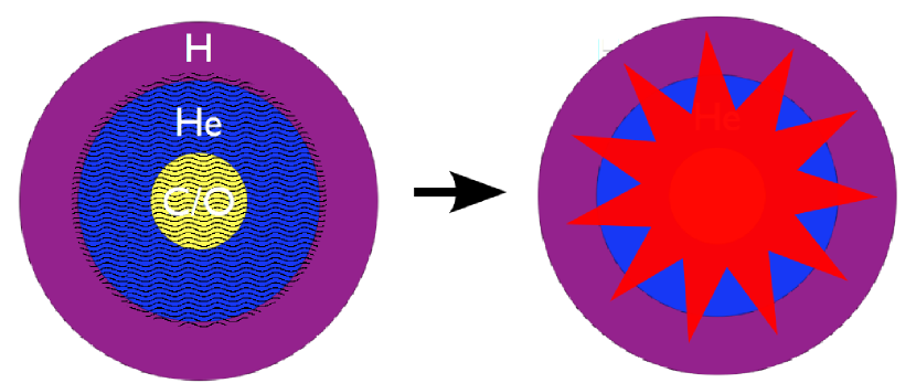
Figure 1: After central helium burning, the helium core of very massive star becomes highly convective (wavy mesh) and radiation energy is converted into electron and positron pairs at its oxygen core; This results in an implosion that ignites the oxygen and silicon explosively. The energy released from burning eventually blows up the star.

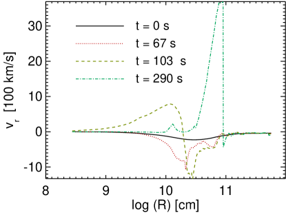
(a) Evolution of radial velocity profiles

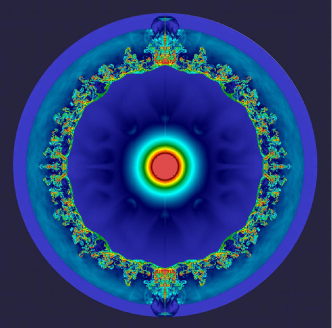
(b) A PSN explosion

Figure 2: (a) The in-falling velocities of collapsing core begin at about $200\,{\mathrm{km}}\sec^{-1}$. After the explosion occurs, a strong shock is launched and will propagate until it breaks out from the stellar surface. (b) The fluid instabilities generated during the explosion evolve into a large spatial scale and generated a significant mixing.

CASTRO [7, 8] is a massively parallel, multidimensional Eulerian adaptive mesh refinement (AMR) radiation-hydrodynamics code for astrophysical applications. Its time integration of the hydrodynamics equations is based on a higher-order, unsplit Godunov scheme. Block-structured AMR with subcycling in time applies high spatial resolution to where it is needed most. We use the Helmholtz equation of state [17] with density, temperature, and elemental abundances; it includes contributions by non-degenerate and degenerate relativistic and non-relativistic electrons, electron-positron pair production, ions and radiation. The gravitational field is calculated with a monopole approximation derived from a radial average of the density on the multidimensional grid. We have implemented several reaction networks (7, 13, 19 isotopes) [5, 18] in CASTRO for calculating nucleosynthesis and energetics in thermonuclear SNe. The most comprehensive network includes alpha-chain reactions, heavy-ion reactions, hydrogen burning cycles, photo-disintegration of heavy elements, and energy loss by neutrinos.

3 Conservative Mapping

Since the star is very nearly in hydrostatic equilibrium and we want to conserve total energy, care must be taken when mapping its profile from the uniform Lagrangian grid in mass coordinate to the new Eulerian spatial grid. Zingale et al. [19], Mocák et al. [20] have also studied mapping 1D initial conditions onto multidimensional grids. Different from our scheme, they focus on maintaining the hydrostatic equilibrium setup, because hydrostatic equilibrium is required for their simulations such as modelling X-ray bursts on the surface of neutron stars. If their initial conditions do not maintain the hydrostatic equilibrium, the strong gravity of neutron stars can rapidly pull down the burning layers and cause artificial heating which leads to problematic results. To construct a hydrostatic equilibrium profile, their mapping can not conserve physical quantities such as mass or internal energy. Instead, our problems start with initial conditions that are not at the hydrostatic equilibrium and the burning time scale is significantly less than the dynamic time scale of the star. The proper temperature and density profiles are more important for our problems. Our method preserves the conservation of quantities such as mass and energy on the new mesh that are analytically conserved in the evolution equations. Figure 2(a) shows the radial velocity evolution of an example of PSN simulations. When $t=0$, $V_{\rm r}$ is nonzero which indicates the initial condition is not hydrostatic equilibrium. Figure 2(b) shows a PSN explosion right before the shock breaks out of the stellar surface.

Although this reconstruction does not guarantee that the star will be hydrostatic, it is a physically motivated constraint and sufficient for our simulations. The algorithm we describe is specific to our models but can be easily generalized to mappings of other 1D data to higher dimensional grids.

3.1 Method

First, we construct a continuous (C⁰) function that conserves the physical quantity upon mapping onto the new grid. An ideal choice for interpolation is the volume coordinate $V$, the volume enclosed by a given radius from the center of the star. Then, integrating a density $\rho_{X}$ (which can represent mass or internal energy density) with respect to the volume coordinate yields a conserved quantity $X$

$$X=\int_{V_{1}}^{V_{2}}\rho_{X}\,\mathrm{d}V,$$ (1)

such as the total mass or total internal energy lying in the shell between $V_{1}$ and $V_{2}$.

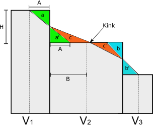
Figure 3: Constructing a piecewise-linear conservative profile: The rectangular bins represent the original 1D profile. The areas of different colors represent conserved quantities such as mass and internal energy. The conservative profile connects adjacent bins and makes a =a^′ = $\frac{1}{4}H\times$ min(A,B), c = c^′, and b = b^′. Note that uniform zones in mass (Lagrangian coordinate) lead to nonuniform bins in volume coordinate, as shown above.

Next, we define a piecewise linear function in volume $V$ that represents the conserved quantity $\rho_{X}$, preserves its monotonicity (no new artificial extrema), and is bounded by the extrema of the original data. The segments are constructed in two stages. First, we extend a line across the interface between adjacent zones that either ends or begins at the center of the smaller of the two zones, as shown in Figure 3 (note that uniform zones in mass coordinate do not result in uniform zones in $V$). The slope of the segment is chosen such that the area trimmed from one zone by the segment (a and b) is equal to the area added under the segment in the neighboring bin (a^′=a and b^′=b).

If the two segments bounding a and a^′, and b and b^′ are joined together by a third in the center zone in Figure 3, two “kinks”, or changes in slope, can arise in the interpolated quantity there; plus, the slope of the flat central segment is usually a poor approximation of the average gradient in that interval. We therefore construct two new segments that span the entire central zone and connect with the two original segments where they cross its interfaces, as shown in Figure 3. The new segments join each other at the position in the central bin where the areas c and c^′ enclosed by the two segments are equal (note that they typically have different slopes). After repeating this procedure everywhere on the grid, each bin will be spanned by two linear segments that represent the interpolated quantity $\rho_{X}$ at any $V$ within the bin and have no more than one kink in $\rho_{X}$ across the zone. Our scheme introduces some smearing (or smoothing) of the data, but it is limited to at most the width of one zone on the original grid. Other approaches might be the use of a parabolic reconstruction, such as that described by the PPM [21], ENO [22], and WENO [23] schemes. However, these schemes aim mainly for problems with piecewise smooth solutions containing discontinuities. Most models of 1D stellar evolution before their supernova explosions do not contain the discontinuities in the profiles of physical quantities such as density and temperature. Hence our scheme offers a simpler and more effective implementation for the conservative profile reconstruction.

The result of our interpolation scheme is a piecewise linear reconstruction in $V$ of the original profile in mass coordinate for which the quantity $\rho_{X}$ can be determined at any $V$, not just the radii associated with the zone boundaries in the Lagrangian grid. We show this profile as a function of the radius associated with the volume coordinate $V$ for a zero-metallicity 200 $\mathrm{M}_{\odot}$ star with $r$ $\sim$ $2\times 10^{13}$ cm from KEPLER [11, 24].

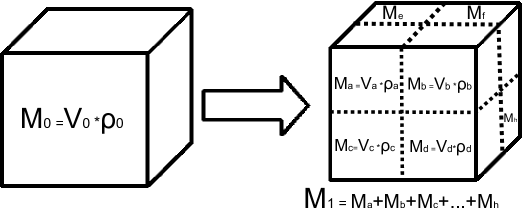
Figure 4: Volume subsampling: We first use the center of volume element (V₀) to obtain its density $\rho_{0}$ from the conservative profile and then calculate its mass M₀ = V${}_{0}\times\rho_{0}$. We then partition the original volume element as shown and calculate the mass of each subvolume in the same manner as M₀. We obtain M₁ by summing over eight subvolumes M_a,M_b,M_c,…,M_h. We then compare M₁ and M₀; if their relative error is greater than some predetermined tolerance the process is recursively repeated until $|$(M_i-M_i-1)/M_i$|$ is less than $10^{-4}$.

We populate the new multidimensional grid with conserved quantities from the reconstructed stellar profiles as follows. First, the distance of the selected mesh point from the center of the new grid is calculated. We then use this radius to obtain its $V$ to reference the corresponding density in the piecewise linear profile of the star. The density assigned to the zone is then determined from adaptive iterative subsampling. This is done by first computing the total mass of the zone by multiplying its volume by the interpolated density. We then divide the zone into equal subvolumes whose sides are half the length of the original zone. New $V$ are computed for the radii to the center of each of these subvolumes and their densities are again read in from the reconstructed profile. The mass of each subvolume is then calculated by multiplying its interpolated density by its volume element (see Figure 4). These masses are then summed and compared to the mass previously calculated for the entire cell. If the relative error between the two masses is larger than the desired tolerance, each subvolume is again divided as before, masses are computed for all the constituents comprising the original zone, and they are then summed and compared to the zone mass from the previous iteration. This process continues recursively until the relative error in mass between the two most recent consecutive iterations falls within an acceptable value, typically 10^-4. The density we assign to the zone is just this converged mass divided by the volume of the entire cell. This method is used to map internal energy density and the partial densities of the chemical species to every zone on the new grid. The total density is then obtained from the sum of the partial densities; pressure, and temperature in turn are determined from the equation of state. This method is easily applied to hierarchy geometry of the target grid.

3.2 Results

We port a 1D stellar model from KEPLER into CASTRO to verify that our mapping is conservative. As an example, we use a 200 $\mathrm{M}_{\odot}$ zero-metalicity pre-supernova star.

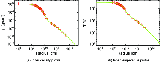
Figure 5: Inner density and temperature profiles of a 200 $\mathrm{M}_{\odot}$ presupernova: Our piecewise linear profiles (green lines) fit their original KEPLER model (red crosses) very well. Since we map internal energy (a conserved quantity) rather than temperature, we calculate $T$ from the equation of state using the density, element abundance, and internal energy.

As we show in Figure 5, our piecewise linear fits to the KEPLER data reproducing the original stellar profile. Because our fits smoothly interpolate the block histogram structure of the KEPLER bins (especially at larger radii), they reduce the number of unphysical sound waves that would have been introduced in CASTRO by the discontinuous interfaces between these bins in the original data. The density profile is key to the hydrodynamic and gravitational evolution of the explosion, and the temperature profile is crucial to the nuclear burning that powers the explosion.

We first map the profile onto a 1D grid in CASTRO and plot the mass of the star as a function of grid resolution in Figure 6. The mass is independent of resolution for our conservative mapping because we subsample the quantity in each cell prior to initializing it, as described above. In contrast, the total mass from linear interpolation is very sensitive to the number of grid points but does eventually converge when the number of zones is sufficient to resolve the core of the star, in which most of its mass resides.

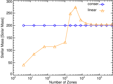
Figure 6: Total mass of the star on the 1D CASTRO grid as a function of number of zones: Conservative mapping (blue) preserves the mass of the star at all resolutions, while linear interpolation (orange) converges to 200 $\mathrm{M}_{\odot}$ at a resolution of $\sim$ a few $\times 10^{4}$, when the grid begins to resolve the core of the star ($\sim 10^{9}$ cm). Even at very high resolutions, the results of linear interpolation are still off by a few percent from the targeted mass and start to be saturated at $\sim 10^{5}$ zones because the linear interpolation profile is not a conservative one.

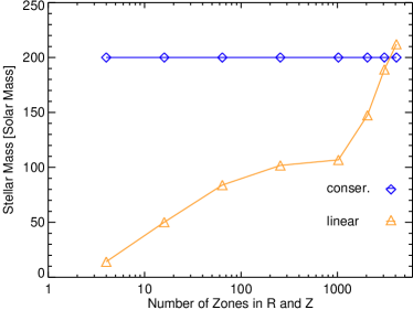
(a) 2D Mapped Mass of Entire Star

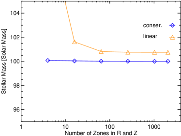
(b) 2D Mapped Mass of Helium Core

Figure 7: (a) Total mass of the star on the new 2D CASTRO grid as a function of number of zones in both $r$ and $z$: Conservative mapping (blue) recovers the mass of the star at all resolutions and linear interpolation (orange) approaches 200 $\mathrm{M}_{\odot}$ at a resolution of $\sim$ $2048^{2}$. (b) Total mass of the He core on the 2D CASTRO grid as a function of number of zones in both $r$ and $z$: Conservative mapping (blue) preserves its original mass at all resolutions while linear interpolation (orange) begins to converge to 100 $\mathrm{M}_{\odot}$ at a resolution of $64^{2}$, but it is still off by $\sim 1\%$ even as the resolution approaches $\sim 2048^{2}$ because the linear interpolation profile is, by nature, not conservative.

We next map the KEPLER profile onto a 2D cylindrical grid ($r,z$) and a 3D cartesian grid ($x,y,z$) in CASTRO. The only difference between mapping to 1D, 2D, and 3D is the form of the volume elements used to subsample each cell, which are $4\pi r^{2}dr$, $2\pi rdrdz$, $dxdydz$, respectively. We show the mass of the star as a function of resolution in Figure 7(a). Conservative mapping again preserves its mass at all grid resolutions. In 2D, more zones are required for linear interpolation to converge to the mass of the star. To further verify our conservative scheme, we map just the helium core of the star ($\sim$ 100 ${\mathrm{M}_{\odot}}$ with $r\sim$ 10¹⁰ cm) onto the 2D grid. The helium core is crucial to modeling thermonuclear supernovae because it is where explosive burning begins. We show its mass as a function of resolution in Figure 7(b). We again recover all the mass of the core at all resolutions because linear interpolation overestimates the mass by at least $\sim$ 1 $\%$, even with large numbers of zones.

Because of the property of reconstruction, conservative mapping is still valid in 3D but requires much more computational time to subsample each cell to convergence. Furthermore, an impractical number of zones is needed for linear interpolation to reproduce the original mass of the star. So we do not show the comparison of 3D models. We note that our method also works with AMR grids because both $V$ and the interpolated quantities can be determined, and subsampling can be performed on every grid in the hierarchy. For the given domain, the results of conservative mapping are independent of the levels of AMR.

4 Initial Perturbation

Seeding the pre-supernova profile of the star with realistic perturbations may be important to understanding how fluid instabilities later erupt and mix the star during the explosion. Massive stars usually develop convective zones prior to exploding as SNe [10, 11]. Multidimensional stellar evolution models suggest that the fluid inside the convective regions can be highly turbulent [12, 13]. However, in lieu of the 3D stellar evolution calculations necessary to produce such perturbations from first principles, multidimensional simulations are usually just seeded with random perturbations. In reality, if the star is convective and the fluid in those zones is turbulent [14], a better approach is to imprint the multidimensional profiles with velocity perturbations with a Kolmogorov energy spectrum [15].

Next we describe our scheme for seeding 2D and 3D stellar profiles with turbulent perturbations and present stellar evolution simulations with CASTRO with these profiles. In our setup, the perturbations have the following properties:

1. The perturbations are imprinted in the gas velocity, and their net momentum flux must be zero. Because the initial perturbations only play as seeds for any fluid instabilities and we want to minimize the overall impact of perturbed velocities to the dynamics of star. $\nabla\cdot(\rho v)=0$ may not be fulfilled locally. So strictly speaking, the perturbed velocity field is not solenoidal.

2. They are seeded in convectively unstable regions with a velocity spectrum $V(k)\sim k^{-5/6}$, where $k$ is the wave number and the power index $-5/6$ is for a Kolmogorov spectrum with an assumption of constant density. We assume a low Mach number convection, which implies that the fluid can be approximated as incompressible, which leads to the density contrast of convective bubbles being small. The 1D MLT of our models also suggest that convective velocities are subsonic.

4.1 2D Perturbation

We first consider the mapping onto a polar coordinate grid in $r$ and $\theta$. To enforce zero net momentum and the boundary conditions in the simulation, we define a new variable $x=1+\cos\theta$ instead of using $\theta$. The momentum flux of a density $\rho$ and velocity $v_{r}$ is then

$$\int_{0}^{\pi}\!2\pi r^{2}\rho v_{r}\sin\theta\,\mathrm{d}\theta=\int_{0}^{2}\!2\pi r^{2}\rho v_{r}\,\mathrm{d}x=0$$ (2)

if $v_{r}$ has the form $\cos(2\pi nx)$, where $n$ is an integer. When $\theta$ = 0, $\pi$ (the boundaries of a 2D grid), $x$ = 2, 0 yields the maximum values for $v_{r}$ that satisfy the boundary conditions in 2D cylindrical coordinates in CASTRO. There are two physical scales that constrain the wavelength of the perturbation in $r$. Based on the mixing length theory [25], the eddy size of turbulence is $\alpha\times H_{\rm p}$; $\alpha$ is the mixing length parameter, and $H_{\rm p}$ is the pressure scale height. Here, we set $\alpha$ = 1.0. Since the perturbation is only seeded in the convective zones, it is confined inside domain $D_{c}=r_{\rm u}$ - $r_{\rm b}$, where $r_{\rm u}$ and $r_{\rm b}$ are its upper and lower boundaries. The maximum wavelength of the perturbation must be smaller than $D_{\rm c}$ and $H_{\rm p}$. Inside a convective zone, we define a new variable, $y=\int_{r_{\rm b}}^{r}\frac{{\rm d}r}{H_{\rm p}(r)}$. We also define two oscillatory functions in $x$ and $y$ to generate the circular patterns that mimic the vortices of a turbulent fluid. Since the fluid inside the convective zone is turbulent, its energy spectrum is $E(k)\sim k^{-5/3}$. Assuming a constant density, the corresponding velocity spectrum is $V(k)\sim k^{-5/6}$. The perturbed velocity then has the form,

$$\begin{array}[]{l}V_{{\rm perb},r}(x,y)=-\sum\limits_{a}\sum\limits_{b}V_{\rm p}\cdot\cos(2\pi ax)\cdot\cos(2\pi by+\alpha_{b}),\\ V_{\rm perb,\theta}(x,y)=\sum\limits_{a}\sum\limits_{b}V_{\rm p}\cdot\sin(2\pi ax)\cdot\cos(2\pi by+\alpha_{b}),\\ V_{\rm p}=V_{\rm d}(r)b^{-5/6},\end{array}$$ (3)

where $V_{{\rm perb},r}$ and $V_{\rm perb,\theta}$ are the perturbed velocities in the $r$ and $\theta$ directions, and $a$ and $b$ are angular and radial wavenumbers. 1D models provide only the information of convective velocities, $V_{\rm d}(r)$ along the radial direction, which can be treated as average velocities of angular directions, so we scale the amplitude of the perturbed velocity based on the radial wavenumber $b$. Besides, we use the oscillatory functions for constructing the eddy-like pattern of perturbed velocity field which provides an alternative way to angularly distribute our perturbation. This is based on a physically motivated way, which is more realistic than purely random perturbations. In a realistic turbulent follow, $V_{\rm p}$ of eddies should depend only on the scale of physical length without preferred direction. In our setup, we simplify the implementation by constraining the length scale only in the radial direction. Our oscillatory functions then decompose $V_{\rm p}$ in $r$, $\theta$, and $\phi$ directions. We also use a random phase, $\alpha_{b}$, to smooth out numerical discontinuities caused by the perturbed modes while summing. Equations (3) by construction satisfy $V_{\rm perb,\theta}(r,\theta)=0$ when $\theta=0$ and $\pi$, the boundary conditions in $\theta$ on the 2D grid. The assumption of no overshooting makes $V_{{\rm perb},r}=0$ at the boundaries of convective zones, so we set $V_{{\rm perb},r}=0$ at boundaries. The ultimate wavenumbers of $a$ and $b$ are also limited by $D_{c}$, $H_{p}$, and the resolution of simulation, $H_{\rm res}$.

4.2 3D Perturbation

In 3D, we use spherical coordinates, $r$, $\theta$, and $\phi$. Similar to 2D, we construct an oscillatory function for ($\theta,\phi$) by using spherical harmonics, $Y_{l,m}(\theta,\phi)$, where $l$ and $m$ are the wavenumbers in $\theta$ and $\phi$. If the velocities are in the form of $Y_{l,m}(\theta,\phi)$, they automatically conserve momentum flux while summing all the modes $l,m$. In the radial direction, we use $\cos(cy)$, where $c$ is the wavenumber in the radial direction and $y$ is as defined in 2D. The perturbation then has the following form:

$$\begin{array}[]{l}V_{{\rm perb},x}(r,\theta,\phi)=V_{\rm perb}\sin(\theta)\cos(\phi),\\ V_{{\rm perb},y}(r,\theta,\phi)=V_{\rm perb}\sin(\theta)\sin(\phi),\\ V_{{\rm perb},z}(r,\theta,\phi)=V_{\rm perb}\cos(\theta),\\ V_{\rm perb}=\sum\limits_{c}\sum\limits_{l}\sum\limits_{m}V_{\rm p}\cdot Y_{l,m}(\theta+\omega_{lm},\phi+\omega_{lm})\cdot\cos(2\pi cy+\lambda_{c}),\\ V_{\rm p}=V_{\rm d}(r)c^{-5/6},\end{array}$$ (4)

where $V_{{\rm perb},x}$, $V_{{\rm perb},y}$, $V_{{\rm perb},z}$ are the perturbed velocities in the $x$, $y$, and $z$ directions. We sum over the modes, applying random phases $\omega_{lm}$ and $\lambda_{c}$ to smooth out numerical discontinuities caused by different perturbed modes. Similar to 2D, $V_{\rm p}$ is only scaled by radial wavenumber $c$. Because there are no reflective boundary conditions for 3D, we only take care of the boundary conditions in radial direction. We again assume there is no overshooting outside the boundaries of convective zones, so we enforce $V_{\rm perb}$ to zero at boundaries.

4.3 Results

We first initialize perturbations on a 2D grid with a profile that is derived from a 1D KEPLER stellar evolution calculation. The perturbations are confined to regions that are convectively unstable [26]. The magnitude $V_{\rm d}(r)$ of the perturbed velocity adopts the diffusion velocity, which is usually $\sim$ $1-10\%$ of the local sound speed. We again consider a zero-metalicity $200\,{\mathrm{M}_{\odot}}$ star in the pre-supernova phase. This star develops a large convection zone that extends out to the hydrogen envelope. We show the magnitude of the perturbed velocity generated by the two oscillatory functions discussed above on our 2D grid in Figure 8(a). The velocity field satisfies the reflecting boundary conditions on the 2D grid at $\theta$ = 0 and $\pi$. In the right panel we show velocity vectors in the selected subregion on the left (blue rectangle). A clear vortex pattern that mimics a turbulent fluid is clearly visible. Next we calculate energy spectrum of perturbed velocity field. We first randomly pick a radial direction ( constant $\theta$ in 2D) or (constant $\theta$ and $\phi$)in 3D) inside the convective zone, perform Fourier transfer of $V_{\rm p}$ along the radial direction, then calculate its power spctrum. We repeat the same process ten times, our final spectrum is obtained by averaging all spectra previously calcuated. $k$ = $H_{\rm p}/l$, where $H_{\rm p}$ is the pressure scale height and $l$ is the physical scale in $r$ direction. Figure 8(b) shows the energy spectrum of the fluid, which is basically a Kolmogorov spectrum $E(k)\sim k^{-5/3}$ except for fluctuations in part caused by the random phases in the sum over modes in $r$, and $V_{\rm d}(r)$ is not a constant across the convective region that produces an offset in the smaller $k$ region. The energies would converge to the Kolmogorov spectrum in the limit of large $k$, but the maximum $k$ of our simulation is limited to the resolution of the grid.

We next port our 1D KEPLER model to a 3D grid. In Figure 9(a), we show a slice of the magnitude of the perturbed velocity, which again exhibits the clear cell pattern reminiscent of the vortices of a turbulent fluid. The velocity pattern in 3D is more irregular than in 2D. We show the energy spectrum of the velocity field in Figure 9(b), which is similar to that of our 2D spectrum but with larger fluctuations that are again due to the random phases we assign to each spherical harmonic, and the $V_{\rm d}(r)$ is not a constant across the convective region that produces an offset in the smaller $k$ region. We also check the values of perturbed velocities whether they are consistent to the $V_{\rm d}(r)$ or not. We calculate the variance of radial velocities; $\delta V_{r}=\langle V(r)-\langle V(r)\rangle\rangle$. Figure 10 shows the comparison between $\delta V_{r}$ and $V_{\rm d}$ as a function of radius. The values of $\delta V_{r}$ are consistent to the original $V_{\rm d}$. The oscillatory pattern of $\delta V_{r}$ comes from our formalism Equations (4). Above examples demonstrate that our scheme effectively generates turbulent fluid perturbations analog to those found in the convective regions of massive stars, with the desired velocity patterns and energy power spectra.

We do not claim the models here can fully reproduce the true turbulence found in simulations or laboratories. Unlike previous multidimensional simulations of this kind, whose initial perturbations were seeded by numerical noises or random perturbations. The scheme here is the first attempt to model the initial perturbations based on a more realistic setup, where the convective zones of a star play an ideal role for generating perturbations. These kinetic energy of these perturbations is very small compared with the internal energy of the gas, thus it does not interfere with the overall dynamics of the simulations or trigger an artificial ignition. We seed initial perturbations to trigger the fluid instabilities on multidimensional simulations so we can study how they evolve with their surroundings as shown in Figure 2(b). When the fluid instabilities start to evolve nonlinearly, the initial imprint of perturbation would be smeared out. The random perturbations and turbulent perturbations then give consistent results. Depending on the nature of problems, the random perturbations might take a longer time to evolve the fluid instabilities into turbulence because more relaxation time is required.

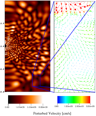
(a) 2D Perturbed Velocity

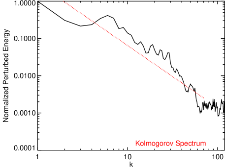
(b) 2D Energy Power Spectrum

Figure 8: (a) 2D perturbed velocity in the interior of the star on physical scales $\sim 10^{12}$ cm: The closeup is the velocity vector field corresponding to the blue rectangle and exhibits a vortex pattern similar to that of a turbulent fluid. (b) Normalized kinetic energy power spectrum of a 2D perturbed field: The dotted red line is the Kolmogorov spectrum, $E(k)\sim k^{-5/3}$. The peak of the Kolmogorov spectrum is adjusted to fit the data. The scale of $H_{p}$ is equaled to $k=1$. The suppressed power at lower $k$ is because of the inhomogeneous of $V_{\rm p}(r)$ at larger scales. The decay trend follows $k^{-5/3}$, and the fluctuations are caused by the radial oscillatory function with random phases.

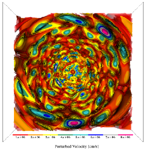
(a) 3D Perturbed Velocity

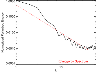
(b) Kinetic Energy Power Spectrum of 3D perturbed field

Figure 9: (a) 3D perturbed velocity field: The iso-surfaces show the magnitude of the perturbed velocity on physical scales of $10^{12}$ cm. (b) Corresponding energy power spectrum: The dotted red line shows the Kolmogorov spectrum, $E(k)\sim k^{-5/3}$. The peak of the Kolmogorov spectrum is adjusted to fit the data. The scale of $H_{p}$ is equaled to $k=1$. Similar to 2D, the decay trend follows $k^{-5/3}$, and the fluctuations are caused by the radial oscillatory function with random phases.

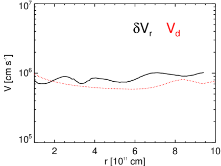
Figure 10: $\delta V_{r}$ and $V_{\rm d}$ as a function $r$ inside the convective zone of the star: The values of $\delta V_{r}$ inside the convective zone are about $10^{6}\,{\mathrm{cm}}\,\sec^{-1}$, those are consistent to the values of $V_{\rm d}$, predicted from the 1D MLT theory. The oscillatory trend of $\delta V_{r}$ reflects the original function form of the perturbations.

5 Resolving the Early Stages of the Explosion

In addition to implementing realistic initial conditions and relevant physics for CASTRO, care must be taken to determine the resolution of multidimensional simulations required to resolve the most important physical scales and yield consistent results, given the computational resources that are available. We provide a systematic approach for finding this resolution for multidimensional stellar explosions.

Simulations that include nuclear burning, which governs nucleosynthesis and the energetics of the explosion, are very different from purely hydrodynamical models because of the more stringent resolution required to resolve the scales of nuclear burning and the onset of fluid instabilities in the simulations. Because energy generation rates due to burning are very sensitive to temperature, errors in these rates as well as in nucleosynthesis can arise in zones that are not fully resolved. We determine the optimal resolution with a grid of 1D models in CASTRO. Beginning with a crude resolution, we evolve the pre-supernova star and its explosion until all burning is complete and then calculate the total energy of the supernova, which is the sum of the gravitational energy, internal energy, and kinetic energy. We then repeat the calculation with the same setup but with a finer resolution and again calculate the total energy of the explosion. We repeat this process until the total energy is converged. As shown in Figure 11, our example of a $200\,{\mathrm{M}_{\odot}}$ presupernova converges when the resolution of the grid approaches $10^{8}\,{\mathrm{cm}}$.

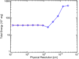
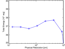
Figure 11: Total explosion energy as a function of resolution: the x-axis is the grid resolution and the y-axis is the total energy, defined to be the sum of the gravitational energy, the internal energy, and the kinetic energy. The total energy is converged when the resolved scale is close to ${10^{8}}$ cm. The right panel shows the zoom-in of the red box in left panel.

The time scales of burning (${\rm d}t_{\rm b}$) and hydrodynamics (${\rm d}t_{\rm h}$) can be very disparate, so we adopt time steps of $min({\rm d}t_{\rm h},{\rm d}t_{\rm b})$ in our simulations, where ${\rm d}t_{\rm h}=\frac{{\rm d}x}{c_{\rm s}+|v|}$; ${\rm d}x$ is the grid resolution, $c_{s}$ is the local sound speed, $v$ is the fluid velocity, and the time scale for burning is ${\rm d}t_{\rm b}$, which is determined by both the energy generation rate and the rate of change of the abundances.

5.1 Homographic Expansion

As we have shown, grid resolutions of $10^{8}\,{\mathrm{cm}}$ are needed to fully resolve nuclear burning in our model. However, the star can have a radius of up to several $10^{14}\,{\mathrm{cm}}$. This large dynamical range (10⁶) makes it impractical to simulate the entire star at once while fully resolving all relevant physical processes. When the shock launches from the center of the star, the shock’s traveling time scale is about a few days, which is much shorter than the Kelvin–Helmholtz time scale of the stars, about several million years. We can assume that when the shock propagates inside the star, the stellar evolution of the outer envelope is frozen. This allows us to trace the shock propagation without considering the overall stellar evolution. Hence, we instead begin our simulations with a coordinate mesh that encloses just the core of the star with zones that are fine enough to resolve explosive burning. We then halt the simulation as the SN shock approaches the grid boundaries, uniformly expand the simulation domain, and then restart the calculation. In each expansion we retain the same number of grids (see Figure 12). Although the resolution decreases after each expansion, it does not affect the results at later times because burning is complete before the first expansion and emergent fluid instabilities are well resolved in later expansions. These uniform expansions are repeated until the fluid instabilities cease to evolve. There might be some possible sound waves generated from boundaries under such a setup. However, the normal SN shocks have a much higher mach number—above 10—while traveling inside the star. The sound waves could not contaminate the burning/fluid instabilities domains before the shock reaches the boundary of the simulation box.

Most stellar explosion problems need to deal with a large dynamic scale such as the case discussed here. It is computationally inefficient to simulate the entire star with a sufficient resolution. Because the time scale of the explosion is much shorter than the dynamic time of stars, we can follow the evolution of the shock by starting from the center of the star and tracing it until the shock breaks out of the stellar surface. The utility of homographic expansion is also available in CASTRO.

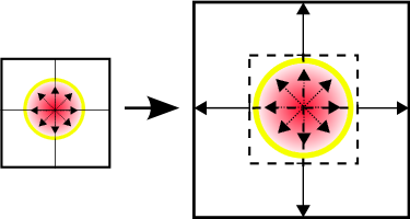
Figure 12: Homographic expansion: In both panels, the yellow circle is the SN shock and the red region is the ejecta. The simulations begin with just the inner part of the star and a higher resolution (left panel) for capturing fluid instabilities and burning. After the explosion occurs, we follow the shock until it reaches the boundary of the simulation box. We then expand the simulation domain, mapping the final state of the previous calculation onto the new mesh with a new ambient medium that is taken from the initial profile.

6 Conclusion

Multidimensional stellar evolution and supernova simulations are numerically challenging because multiple physical processes (hydrodynamics, gravity, burning) occur on many scales in space and time. For computational efficiency, 1D stellar models are often used as initial conditions in 2D and 3D calculations. Mapping 1D profiles onto multidimensional grids can introduce serious numerical artifacts, one of the most severe of which is the violation of conservation of physical quantities. We have developed a new mapping algorithm that guarantees that conserved quantities are preserved at any resolution and it reproduces the most important features in the original profiles. Our method is practical for 1D and 2D calculations, and we plan to develop integral methods (an explicit integral approach instead of using volume subsampling) that are numerically tractable in 3D.

Multidimensional models give insight on fluid instabilities in supernova explosions that break the spherical symmetry of stars and mix their interiors. These instabilities originate from perturbations in the star prior to the explosion. Until now, these perturbations have been randomly seeded in 2D and 3D models with little or no physical basis. We present a new approach to seeding supernova models with physically realistic velocity perturbations like those found in the turbulent convective zones of massive stars. We find that the initial spectrum of the perturbations tends to be smeared out as they become nonlinear. Our approach can be applied to other multidimensional simulations of stellar explosions, especially those whose final outcomes are sensitive to the form of the initial perturbation; or the simulations of short duration, in which perturbations may not become fully nonlinear.

Finally, we provide possible approaches to obtain the proper resolution for simulations that include both hydrodynamics and nuclear burning. Because the burning changes both the internal energy and composition of the fluid, we determine the physical scale for resolving burning with resolution tests and proper time steps by considering both hydro and burning. We apply a homographic expansion to bypass the numerical difficulties associated with the large range of dynamical scales in our problem. The algorithms we present can be applied to other multidimensional simulations in addition to stellar explosions in both astrophysics and cosmology.

References

- Herant and Woosley [1994] M. Herant, S. E. Woosley, ApJ 425 (1994) 814–828.
- Joggerst et al. [2009] C. C. Joggerst, S. E. Woosley, A. Heger, ApJ 693 (2009) 1780–1802.
- Joggerst et al. [2010] C. C. Joggerst, A. Almgren, J. Bell, A. Heger, D. Whalen, S. E. Woosley, ApJ 709 (2010) 11–26.
- Joggerst and Whalen [2011] C. C. Joggerst, D. J. Whalen, ApJL 728 (2011) 129.
- Weaver et al. [1978] T. A. Weaver, G. B. Zimmerman, S. E. Woosley, ApJ 225 (1978) 1021–1029.
- Paxton et al. [2011] B. Paxton, L. Bildsten, A. Dotter, F. Herwig, P. Lesaffre, F. Timmes, ApJS 192 (2011) 3.
- Almgren et al. [2010] A. S. Almgren, V. E. Beckner, J. B. Bell, M. S. Day, L. H. Howell, C. C. Joggerst, M. J. Lijewski, A. Nonaka, M. Singer, M. Zingale, ApJ 715 (2010) 1221–1238.
- Zhang et al. [2011] W. Zhang, L. Howell, A. Almgren, A. Burrows, J. Bell, ApJS 196 (2011) 20.
- Fryxell et al. [2000] B. Fryxell, K. Olson, P. Ricker, F. X. Timmes, M. Zingale, D. Q. Lamb, P. MacNeice, R. Rosner, J. W. Truran, H. Tufo, ApJS 131 (2000) 273–334.
- Woosley et al. [2002] S. E. Woosley, A. Heger, T. A. Weaver, Reviews of Modern Physics 74 (2002) 1015–1071.
- Heger and Woosley [2002] A. Heger, S. E. Woosley, ApJ 567 (2002) 532–543.
- Porter and Woodward [2000] D. H. Porter, P. R. Woodward, ApJS 127 (2000) 159–187.
- Arnett and Meakin [2011] W. D. Arnett, C. Meakin, ApJ 733 (2011) 78.
- Davidson [2004] P. A. Davidson, Turbulence : an introduction for scientists and engineers, Oxford University Press, 2004.
- Frisch [1995] U. Frisch, Turbulence. The legacy of A. N. Kolmogorov., Cambridge University Press, 1995.
- Barkat et al. [1967] Z. Barkat, G. Rakavy, N. Sack, Physical Review Letters 18 (1967) 379–381.
- Timmes and Swesty [2000] F. X. Timmes, F. D. Swesty, ApJS 126 (2000) 501–516.
- Timmes [1999] F. X. Timmes, ApJS 124 (1999) 241–263.
- Zingale et al. [2002] M. Zingale, L. J. Dursi, J. ZuHone, A. C. Calder, B. Fryxell, T. Plewa, J. W. Truran, A. Caceres, K. Olson, P. M. Ricker, K. Riley, R. Rosner, A. Siegel, F. X. Timmes, N. Vladimirova, ApJS 143 (2002) 539–565.
- Mocák et al. [2009] M. Mocák, E. Müller, A. Weiss, K. Kifonidis, A&A 501 (2009) 659–677.
- Colella and Woodward [1984] P. Colella, P. R. Woodward, Journal of Computational Physics 54 (1984) 174–201.
- Harten et al. [1987] A. Harten, B. Engquist, S. Osher, S. R. Chakravarthy, Journal of Computational Physics 71 (1987) 231.
- Liu et al. [1994] X.-D. Liu, S. Osher, T. Chan, Journal of Computational Physics 115 (1994) 200–212.
- Heger and Woosley [2010] A. Heger, S. E. Woosley, ApJ 724 (2010) 341–373.
- Cox and Giuli [1968] J. P. Cox, R. T. Giuli, Principles of stellar structure, Gordon and Breach, 1968.
- Heger et al. [2000] A. Heger, N. Langer, S. E. Woosley, Apj 528 (2000) 368–396.