Succinct Indices for Range Queries with applications to Orthogonal Range Maxima

Abstract

We consider the problem of preprocessing $N$ points in 2D, each endowed with a priority, to answer the following queries: given a axis-parallel rectangle, determine the point with the largest priority in the rectangle. Using the ideas of the effective entropy of range maxima queries and succinct indices for range maxima queries, we obtain a structure that uses $O(N)$ words and answers the above query in $O(\lg N\lg\lg N)$ time. This is a direct improvement of Chazelle’s result from 1985 [11] for this problem – Chazelle required $O(N/\epsilon)$ words to answer queries in $O((\lg N)^{1+\epsilon})$ time for any constant $\epsilon>0$.

1 Introduction

Range searching is one of the most fundamental problems in computer science with important applications in areas such as computational geometry, databases and string processing. The input is a set of $N$ points in general position in $\mathbb{R}^{d}$ (we focus on the case $d=2$), where each point is associated with satellite data, and an aggregation function defined on the satellite data. We wish to preprocess the input to answer queries of the following form efficiently: given any 2D axis-aligned rectangle $R$, return the value of the aggregation function on the satellite data of all points in $R$. Researchers have considered range searching with respect to diverse aggregation functions such as emptiness checking, counting, reporting, minimum/maximum, etc. [18]. In this paper, we consider the problem of range maximum searching (the minimum variant is symmetric), where the satellite data associated with each point is a numerical priority, and the aggregation function is “arg max”, i.e., we want to report the point with the maximum priority in the given query rectangle. This aggregation function is the canonical one to study, among those of the “commutative semi-group” class [13, 11].

Our primary concern is the space requirement of the data structure — we aim for linear-space data structures, namely those that occupy $O(N)$ words — and seek to minimize query time subject to this constraint. The space usage is a fundamental concern in geometric data structures due to very large data volumes; indeed, space usage is a main reason why range searching data structures like quadtrees, which have poor worst-case query performance, are preferred in many practical applications over data structures such as range trees, which have asymptotically optimal query performance. Space efficient solutions to range searching date to the work of Chazelle [11] over a quarter century ago, and Nekrich [19] gives a nice survey of much of this work. Recently there has been a flurry of activity on various aspects of space-efficient range reporting, and for some aggregation functions there has even been attention given to the constant term within the space usage [5, 19].

We now formalize the problem studied by our paper, as well as those of [11, 9, 16]. We assume input points are in rank space: the $x$-coordinates of the $n$ points are $\{0,\ldots,N-1\}=[N]$, and the $y$-coordinates are given by a permutation $\upsilon:[N]\rightarrow[N]$, such that the points are $(i,\upsilon(i))$ for $i=0,\ldots,N-1$. The priorities of the points are given by another permutation $\pi$ such that $\pi(i)$ is the priority of the point $(i,\upsilon(i))$. The reduction to rank space can be performed in $O(\lg N)$ time with a linear space structure even if the original and query points are points in $\mathbb{R}^{2}$ [13, 11]. The query rectangle is specifed by two points from $[N]\times[N]$ and includes the boundaries (see Fig. 1(R)). Analogous to previous work, we also assume the word-RAM model with word size $\Theta\left(\lg N\right)$ bits.

     

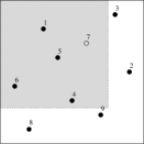
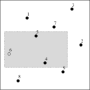
Figure 1: 2-sided and 4-sided range maximum queries. The numbers with the points represent their priorities, and the unshaded points are the answers.

Range maximum searching is a well-studied problem (see Table 1). Chazelle [11] gave a few space/time tradeoffs covering a broad spectrum. To the best of our knowledge, the solution with the lowest query time that uses only $O(N)$ words is still that of Chazelle [11], who gave a query time that is polylogarithmic in $N$. More precisely, he gave a data structure of size $O(\frac{1}{\epsilon}N)$ words with query time $O(\lg^{1+\epsilon}N)$ for any fixed $\epsilon>0$. Other recent results on the range maximum problem are as follows. Karpinski et al. [16] studied the problem of 3D five-sided range emptiness queries which is closely related to range maximum searching in 2D. As observed in [9], their solution yields a query time of $(\lg\lg N)^{O(1)}$ with an index of size $N(\lg\lg N)^{O(1)}$ words. Chan et al. [9] currently give the best query time of $O\left(\lg\lg N\right)$, but this is at the expense of using $O\left(N\lg^{\epsilon}N\right)$ words, for any fixed $\epsilon>0$. However, there has been no improvement in the running time for linear-space data structures. In this paper, we improve Chazelle’s long-standing result by giving a data structure of $O(N)$ words and reducing the query time from polylogarithmic to “almost” logarithmic, namely, $O\left(\lg N\lg\lg N\right)$.

Citation	Size (in words)	Query time
Chazelle’88 [11]	$O\left(N\lg^{\epsilon}N\right)$	$O\left(\lg N\right)$
Chan et al.’10 [9]	$O\left(N\lg^{\epsilon}N\right)$	$O\left(\lg\lg N\right)$
Karpinski et al.’09 [16]	$O\left(N(\lg\lg N)^{O(1)}\right)$	$O\left((\lg\lg N)^{2}\right)$
Chazelle’88 [11]	$O\left(N\lg\lg N\right)$	$O\left(\lg N\lg\lg N\right)$
Chazelle’88 [11]	$O\left(\frac{1}{\epsilon}N\right)$	$O\left(\lg^{1+\epsilon}N\right)$
NEW	$O\left(N\right)$	$O\left(\lg N\,\lg\lg N\right)$

Table 1: Space/time tradeoffs for 2D range maximum searching in the word RAM.

Although our primary focus is on 4-sided queries, which specify a rectangle that is bounded from all sides, we also need to consider 2-sided and 3-sided queries, which are “open” on two and one side respectively (thus a 2-sided query is specified by a single point $(i,j)$—see Fig. 1(L)—and a 3-sided query by two points $(i,j)$ and $(k,l)$ where either $i=k$ or $j=l$). Our solution recursively divides the points into horizontal and vertical slabs, and a query rectangle is decomposed into smaller 2-sided, 3-sided, and 4-sided queries. A key intermediate result is the data structure for 2-sided queries. The 2-sided sub-problems are partitioned into smaller sub-problems, which are stored in a “compressed” format that is then “decompressed” on demand. The “compression” uses the idea that to answer 2-sided range maxima queries on a problem of size $m$, one need not store the entire total order of priorities using $\Theta\left(m\lg m\right)$ bits: $O\left(m\right)$ bits suffice, i.e., the effective entropy [14] of 2-sided queries is low. This does not help immediately, since $\Theta\left(m\lg m\right)$ bits are needed to store the coordinates of the points comprising these sub-problems: to overcome this bottleneck we use ideas from succinct indices [2] — namely, we separate the storage of point coordinates from the data structure for answering range-maximum queries. The latter data structure does not store point coordinates but instead obtains them as needed from a global data structure.

We solve 3-sided and 4-sided subqueries by recursion, or by using structures for range maximum queries on matrices [22, 6]. When recursing, we cannot afford the space required to store the structures for rank space reduction for each such subproblem: a further key idea is to use a single global structure to map references to points within recursive subproblems back to the original points.

By reusing ideas from the data structure for 2-sided queries, we obtain two stand-alone results on succinct indices for 2-sided range maxima queries. In a succinct index, we wish to answer queries on some data, and it is assumed that the succinct index is not charged for the space required to store the data itself, but only for any additional space it requires to answer the queries. However, the succinct index can access the data only through a specific interface (see [2] for a discussion of the advantages of succinct indices). In our case, given $N$ points in rank space, together with priorities, we wish to answer 2-sided range-maximum queries under the condition that the point coordinates are stored “elsewhere”—the data structure is not “charged” for the space needed to store the points “elsewhere”—and are assumed to be available to the data structure in one of two ways:

• Through an orthogonal range reporting query. Here, we assume that a query that results in $k$ points being reported takes $T(N,k)$ time. We assume that $T$ is such that $T(N,O(k))=O(T(N,k))$.

• As in Bose et al. [4], we assume that the point coordinates are stored in read-only memory, permitting random access to the coordinates of the $i$-th point. However, the ordering of the points is specified by the data structure, which we call the permuted-point model.

In both cases, we are able to achieve $O(N)$-bit indices with fast query time, namely $O(\lg\lg N\cdot(\lg N+T(N,\lg N)))$ time, and $O(\lg\lg N)$ time, respectively.

The paper is organized as follows. We first describe some building blocks used in Section 2. Section 3 is devoted to our main result, and Section 4 describes the succinct index results.

2 Preliminaries

Our result builds upon a number of relatively new results, all of which are essential in one way or the other to obtain the final bound. In order to support mapping between recursive sub-problems, we use the following primitives on a set $S$ of $N$ points in rank space. A range counting query reports the number of points within a query rectangle:

Lemma 1 ([15])

Given a set of $N$ points in rank space in two dimensions, there is a data structure with $O(N)$ words of space that supports range counting queries in $O\left(\lg N/\lg\lg N\right)$ time.

A range reporting structure supports the operation of listing the coordinates of all points within a query rectangle. We use the following consequence of a result of Chan et al. [9]:

Lemma 2 ([9])

Given a set of $N$ points in rank space in two dimensions, there is a data structure with $O(N)$ words of space that supports range reporting queries in $O\left((1+k)\lg^{1/3}N\right)$ time where $k$ is the number of points reported.

The range selection problem is as follows: given an input array $A$ of size $N$, to preprocess it so that given a query $(i,j,k)$, with $1\leq i\leq j\leq N$, we return an index $i_{1}$ such that $A[i_{1}]$ is the $k$-th smallest of the elements in the subarray $A[i],A[i+1],\ldots,A[j]$.

Lemma 3 ([7])

Given an array of size $N$, there is a data structure with $O(N)$ words of space that supports range selection queries in $O(\lg N/\lg\lg N)$ time.

3 The data structure

In this section we show our main result:

Theorem 3.1

Given $N$ points in two-dimensional rank space, and their priorities, there is a data structure that occupies $O(N)$ words of space and answers range maximum queries in $O(\lg N\lg\lg N)$ time.

We first give an overview of the data structure. We begin by storing all the points (using their input coordinates) once each in the structures of Lemmas 1 and 2. We also store an instance of the data structure of Lemma 3 once each for the arrays $X$ and $Y$, where $X[i]=\nu(i)$ and $Y[i]=\nu^{-1}(i)$ for $i\in N$ ($X$ stores the $y$-coordinates of the points in order of increasing $x$-coordinate, and $Y$ the $x$-coordinates in order of increasing $y$-coordinate). These four “global” data structures use $O(N)$ words of space in all.

We recursively decompose the problem à la Afshani et al. [1]. Let $n$ be the recursive problem size (initially $n=N$). Given a problem of size $n$, we divide the problem into $n/k$ mutually disjoint horizontal slabs of size $n$ by $k$, and $n/k$ mutually disjoint vertical slabs of size $k$ by $n$. A horizontal and vertical slab intersect in a square of size $k\times k$. We recurse on each horizontal or vertical slab: observe that each horizontal or vertical slab has exactly $k$ points in it, and is treated as a problem of size $k$—i.e. it is logically comprised of two permutations $\upsilon$ and $\pi$ on $[k]$ (Fig. 2(L); Sec. 3.1). Clearly, given a slab in a problem of size $n$ containing $k$ points, we require some kind of mapping between the coordinates in the slab (which in one dimension will be from $[n]$) and the recursive problem in order to view the slab as a problem of size $k$. A key to the space-efficiency of our data structure is that this mapping is not explicitly stored, and is achieved through a slab-rank operation. The slab-select problem is a generalization of the inverse of the slab-rank problem (Sec. 3.2).

The given query rectangle is decomposed into a number of disjoint 2-sided, 3-sided and 4-sided queries, based upon the decomposition of the input into slabs. There are three kinds of terminal queries which do not generate further recursive problems: all 2-sided queries are terminal, 4-sided queries whose sides are slab boundaries are terminal, and all queries that reach slabs at the bottom of the recursion are terminal. The problems (or data structures) that involve answering terminal queries (or are used to answer terminal queries) are also termed terminal. Each terminal query produces some candidate points: the set of all candidate points must contain the final answer. A key invariant needed to achieve the space bound is that all terminal problems of size $n$—except those at the bottom of the recursion—use space $o(n\lg n)$ bits (Sec. 3.1).

Clearly, since storing the input permutation representing the point sets in terminal problems takes $\Theta(n\lg n)$ bits, we do not store them explicitly. Instead, the terminal data structures are succinct indices—the points that comprise them are accessed by means of queries to a single global data structure. The terminal 4-sided problems use an index due to [6], while the 2-sided problems reduce the range maximum query to planar point location. Although there is a succinct index for planar point location [4], this essentially assumes that the points that comprise the planar subdivision are stored explicitly (“elsewhere”) and permuted in a manner specified by their data structure. In our case, if the points are represented explictly, they would occupy $\Theta(N\lg N/\lg\lg N)$ words across all recursive problems. A key to our approach is an implicit representation of the planar sub-division in the recursive problems, relevant parts of which are recomputed from a “compressed” representation at query time (Sec. 3.4); the other key step is to note that $O(n)$ bits suffice to encode the priority information needed to answer 2-sided queries in a problem of size $n$ (Sec. 3.3).

3.1 A recursive formulation and its space usage

The recursive structure is as follows. Let $L=\lg N$, and consider a recursive problem of size $n$ (at the top level $n=N$). We assume that $N$ is a power of 2, as are a number of expressions which represent the size of recursive problems. This can readily be achieved by replacing real-valued parameters $x\geq 1$ by $2^{\lfloor\lg x\rfloor}$ or $2^{\lceil\lg x\rceil}$ without affecting the asymptotic complexity. Unless we have reached the bottom of the recursion, we partition the input range $[n]\times[n]$ into mutually disjoint vertical slabs of width $k=\sqrt{nL}$ and also into mutually disjoint horizontal slabs of height $k=\sqrt{nL}$ – each such slab contains $k$ points and can be logically viewed as a recursive problem of size $k$ (see Fig. 2(L)). Observe that the input is divided into $(n/k)^{2}=n/L$ squares of size $k\times k$, each representing the intersection of a horizontal slab with a vertical one. We need to answer either 2-sided, 3-sided or 4-sided queries on this problem.

The data structures associated with the current recursive problem are:

• for problems at the bottom of the recursion, we store an instance of Chazelle’s data structure which uses $O\left(n\lg n\right)$ bits of space and has query time $O\left((\lg n)^{2}\right)$.

• For 2-sided queries (which are terminal) in non-terminal problems we use the data structure with space usage $O(n\sqrt{\lg n})$ bits described in Sec. 3.4.

• 3- and 4-sided queries, all of whose sides are slab boundaries, are square-aligned: they exactly cover a rectangular sub-array of squares. For such queries, we use a $O(n)$-bit data structure comprising.

  • A $n/k\times n/k$ matrix containing the (top-level) $x$ and $y$ coordinates and priority of the maximum point (if any) in each square. This uses $O(n/L\cdot L)=O(n)$ bits.

  • The data structure of [22, 6] for answering 2D range maximum queries on the elements in the above matrix. This also uses $O(n)$ bits.

Finally, each recursive problem has $O(\lg N)=O(L)$ bits of “header” information, containing, e.g., the bounding box of the problem in the top-level coordinate system. Ignoring the header information, the space usage is given by:

$$S(n)=2\sqrt{n/L}S(\sqrt{nL})+O(n\sqrt{\lg n}),$$

which after $r$ levels of recursion becomes:

$$S(N)=2^{r}\frac{N^{1-1/2^{r}}}{L^{1-1/2^{r}}}S(N^{1/2^{r}}L^{1-1/2^{r}})+O\left(2^{r}N\sqrt{\lg(N^{1/2^{r}}L^{1-1/2^{r}})}\right).$$

The recursion is terminated for the first level $r$ where $2^{r}\geq\lg N/\lg\lg N$. At this level, the problems are of size $O\left((\lg N)^{2}\right)$ and $\Omega\left((\lg N)^{1.5}\right)$ and the second term in the space usage becomes $O(N\lg N)$ bits. Applying $S(n)=O(n\lg n)$ for the base case, we see that the first term is $O((\lg N/\lg\lg N)\cdot N\cdot\lg\lg N)=O(N\lg N)$ bits, and the space used by the header information is indeed negligible.

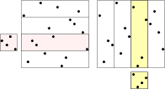
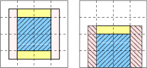
Figure 2: The recursive decomposition of the input (L) and queries (R). In (R), shaded problems are terminal problems. The 4-sided query is decomposed into a square-aligned 4-sided query in the middle and four recursive 3-sided queries, two in horizontal slabs and two in vertical slabs. The 3-sided query is decomposed into two 2-sided queries in vertical slabs, a square-aligned 3-sided query and one recursive 3-sided query in a horizontal slab.

We now discuss the time complexity. In general, we have to answer either 2-sided, 3-sided or 4-sided queries on a slab. Note that (see Fig. 2(R)):

• A 2-sided query is terminal and generates one candidate.

• A 3-sided query results in at most one recursive 3-sided query on a slab (generating no candidates) at most two 2-sided queries on slabs, and at most one square-aligned 3-sided query (generating one candidate).

• A 4-sided query either results in a recursive 4-sided query on a slab (generating no candidates) or generates at most one square-aligned 4-sided query (generating one candidate), plus up to four 3-sided queries in slabs.

Since each 3-sided query only generates one recursive 3-sided query, the number of recursive problems solved, and hence the number of candidates, is $O(r)=O(\lg\lg N)$. The time complexity will depend on the cost of mapping query points and candidates between the problems and their recursive sub-problems and the cost of solving the terminal problems; the former is discussed next.

3.2 The slab-rank and slab-select problems

The input to each recursive problem of size $n$ is given in local coordinates (i.e. from $[n]\times[n]$). Upon decomposing the query to this problem, we need to solve the following slab-rank problem (with a symmetric variant for vertical slabs):

Given a point $p=(i^{*},j^{*})$ in top-level coordinates, which is mapped to $(i,j)$ in a recursive problem of size $n$, such that $(i,j)$ that lies in a horizontal slab of size $n\times k$, map $(i,j)$ to the appropriate position $(i^{\prime},j^{\prime})$ in the size $k$ problem represented by this slab.

We formalize the “inverse” slab-select problem as follows:

Given a rectangle $R$ in the coordinate system of a recursive problem, return the top-level coordinates of all points that lie within $R$.

The following lemma assumes and builds upon the four “global” data structures mentioned after the statement to Theorem 3.1.

Lemma 4

The slab-rank problem can be solved in $O(\lg N/\lg\lg N)$ time, and the slab-select problem in $O(\lg N/\lg\lg N)$ time as well, provided that $R$ contains at most $O\left(\sqrt{\lg N}\right)$ points.

Proof

We first consider the slab-rank problem. Without loss of generality, assume that the given $(i,j)$ is in a horizontal $n\times k$ slab. To translate $j$ to $j^{\prime}$, we only need to subtract the appropriate multiple of $k$ in $O(1)$ time. To map $i$ to $i^{\prime}$, we need to count the number of points in the slab with $x$-coordinate smaller than $i$ (see Fig. 3(L)). Since the top-level coordinates of the point $(i,j)$ are known, and the top-level coordinates of the slab are also stored in the “header” of the slab by assumption, top-level coordinates of all sides of the query are known. As all input points are stored in a global instance of the data structure of Lemma 1, counting the number of points can be performed by an orthogonal range counting query in $O(\lg N/\lg\lg N)$ time.

        

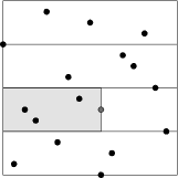
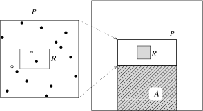
Figure 3: Slab-rank (left) and slab-select (right).

The slab-select problem is solved in a similar manner, and is most easily explained with reference to Fig. 3(R). We are given a recursive sub-problem $P$ and a rectangle $R$ within $P$, and we know $P$’s bounding box in the top-level problem (as shown on the far right). Our aim is to retrieve the top-level coordinates of the image of $R$ in the top-level problem. Suppose that the local $x$ and $y$ coordinates of $R$ are $x_{l}$, $x_{r}$, $y_{b}$ and $y_{t}$. Then we perform a orthogonal range count (Lemma 1) in the area $A$, which lies under $P$ but within $P$’s $x$-coordinates. This takes $O(\lg N/\lg\lg N)$ time, and let $z$ be the value returned. We then select the $z+y_{b}$ and $z+y_{t}$-th smallest $y$-coordinates within $X[x_{l}],\ldots,X[x_{r}]$ by Lemma 3, also taking $O(\lg N/\lg\lg N)$ time. The (top-level) $y$-coordinates of the points returned (shown shaded in the middle) are $R$’s boundaries in the top-level coordinate system. A similar query on $Y[y_{b}],\ldots,Y[y_{t}]$ gives the other boundaries of $R$ in the top-level coordinate system. The $O\left(\sqrt{\lg N}\right)$ points in this rectangle are then retrieved in $O\left((\lg N)^{5/6}\right)=o(\lg N/\lg\lg N)$ time by Lemma 2.

∎

Remark 1

In all applications of the slab-rank result, the top-level coordinates of $(i,j)$ will be known, as $(i,j)$ will either be a vertex of the original input query, or is the result of intersecting a horizontal (or vertical) line through the vertex of a recursive problem (whose top-level coordinates are inductively known) with a vertical (or horizontal) line defining a recursive sub-problem.

3.3 Encoding 2-sided queries

In this section we show Lemma 5. Although the reduction of 2-sided range maxima queries at point $q$ ($RMQ(q)$ hereafter) to orthogonal planar point location is not new, the observation about the amount of priority information needed to answer $RMQ$ is new (and essential). This lemma shows that although storing the permutation $\pi$ itself requires $\Theta(n\lg n)$ bits, the “effective entropy” [14] of the permutation with respect to 2-sided range maximum queries is much lower, generalizing the equivalent statement regarding 1D range-maximum queries [12, 21].

Lemma 5

Given a set $S$ of $n$ points from $\mathbb{R}^{2}$ and relative priorities given as a permutation $\pi$ on $[n]$, the query $RMQ(q)$ can be reduced to point location of $q$ in a collection of at most $n$ horizontal semi-open line segments, whose left endpoints are points from $S$, and whose right endpoints have $x$-coordinate equal to the $x$-coordinate of some point from $S$. Further, given at most $2(n-r)+\lg{{n}\choose{r}}\leq 3n$ bits of extra information, the collection of line segments can be reconstructed from $S$, where $r$ is the number of redundant points—those that are never the answer to any query—in $S$, and this bound is tight.

Proof

Assume the points are in general position and that the 2-sided query is open to the top and left. Associate each point $p=(x(p),y(p))\in S$ with a horizontal semi-open line of influence, possibly of length zero, whose left endpoint (included in the line) is $p$ itself, and is denoted by $\mathit{Inf}(p)$, and contains all points $q$ such that $y(q)=y(p)$, $x(q)\geq x(p)$ and $RMQ(q)=p$. It can be seen that (see e.g. [17]) the answer to $RMQ(q)$ for any $q\in\mathbb{R}^{2}$ can be obtained by shooting a vertical ray upward from $q$ until the first line $\mathit{Inf}(p)$ is encountered; the answer to $RMQ(q)$ is then $p$ (if no line is encountered then there is no point in the 2-sided region specified by $q$). See Fig. 4 for an example.

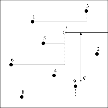
Figure 4: (Left) Example for Lemma 5. The horizontal lines are the lines of influence. Vertical dotted lines show where a point has terminated the line of influence of another point. The arrow shows how point location in the lines of influence answers the 2-sided query with lower right hand corner at $q$, returning the point with priority 7. (Right) Example showing tightness of space bound — points along the diagonal are $A_{\ell}$ and the queries at $p$ and $q$ illustrate how 1D RMQ queries can be answered and redundancy of elements tested, respecitvely.

The set $\mathit{Inf}(S)=\{\mathit{Inf}(p)|p\in S\}$ can be computed by sweeping a vertical line from left to right. At any given position $x=t$ of the sweep line, the sweep line will intersect $\mathit{Inf}(S^{\prime})$ for some set $S^{\prime}$ (initially $S^{\prime}=\emptyset$). If $S^{\prime}=p_{i_{1}},\ldots,p_{i_{r}}$ such that $y(p_{i_{1}})>\ldots>y(p_{i_{r}})$ then it follows that $\pi(i_{1})<\ldots<\pi(i_{r})$ (the current lines of influence taken from top to bottom represent points with increasing priorities). Upon reaching the next point $p_{s}$ such that $y(p_{i_{j}})<y(p_{s})<y(p_{i_{j+1}})$, either (i) $\pi(s)<\pi(i_{j})$—in this case $\mathit{Inf}({p_{s}})$ is empty—or (ii) $\pi(k)>\pi(i_{j})$. In the latter case, it may be that $\pi(k)>\pi(i_{j+1}),\ldots\pi(i_{j+k})$ for some $k\geq 0$, which would mean that $\mathit{Inf}(p_{i_{j+1}}),\ldots,\mathit{Inf}(p_{i_{j+k}})$ are terminated, with their right endpoints being $x(p_{s})$. To construct $\mathit{Inf}(S)$, therefore, only $O(n)$ bits of information are needed: for each point, one bit is needed to indicate whether case (i) or (ii) holds, and in the latter case, the value of $k$ needs to be stored. However, $k$ can be stored in unary using $k+1$ bits, and the total value of $k$, over the course of the entire sweep, is at most $(n-r)$, giving a total of at most $2(n-r)$ bits. The bit-string that indicates whether case (i) or (ii) holds can be stored in $\left\lceil\lg{{n}\choose{n-r}}\right\rceil\leq n$ bits.

To show that this is tight, we consider the 1D range maximum with redundant entries problem, defined as follows. Given an array $A$ of size $n$, of which $r$ entries are redundant, answer the following two queries: firstly, given an index $i$, state whether $A[i]$ is redundant, and secondly, given indices $1\leq i\leq j\leq n$, return the index of the largest value in a query interval $A[i],\ldots,A[j]$ (ignoring redundant values). Given $n,r$, it is easy to see that $2(n-r)+\lg{{n}\choose{r}}-O(\lg n)$ bits are required to encode the answers to the above queries, namely, to answer these queries without accessing $A$. This is because there are ${{n}\choose{r}}$ choices for the positions of the redundant elements, and for each choice of the positions of the redundant elements there are $C_{n-r}=\frac{1}{n-r+1}{{2(n-r)}\choose{n-r}}$ partial orders among the values in $A$ that can be distinguished by 1D range maximum queries [12, 21]. We associate the values in $A$ with a set of $n$ points $A_{\ell}$ placed on a slanted line (in increasing $x$-coordinate order), and give each point in $A_{\ell}$ a priority equal to the corresponding entry in $A$. The point associated with each redundant value in $A$ is given a priority of $-\infty$. In addition we place an $n+1$st point $z$ that dominates all of the points in $A_{\ell}$ (and hence is included in any query that also includes a point from $A_{\ell}$), whose priority is greater than $-\infty$ but less than the smallest priority associated with a non-redundant entry of $A$ (see Fig. 4(R)). The 1D range maximum query problem with redundant entries can can be solved via 2-sided 2D range maximum queries that include only $z$ and the appropriate sub-range of $A_{\ell}$. Also, we can determine if an entry in $A$ is redundant by making a 2-sided query that includes only the corresponding point from $A_{\ell}$ and $z$; the point is redundant iff the answer to such a query is $z$. ∎

Remark 2

It can be shown that $2(n-r)+\lg{{n}\choose{r}}\leq n\lg 5+o(n)$, which is at most $2.33n$ bits for large $n$.

3.4 Data structures for 2-sided queries

In this section we show the following lemma:

Lemma 6

Given a recursive sub-problem of size $n$, we can answer 2-sided queries on this problem in $O(\lg N)$ time using $O(n\sqrt{\lg n})$ bits of space.

This lemma assumes and builds upon the four “global” data structures metioned after the statement to Theorem 3.1. We view the given problem of size $n$, on which we need to support 2-sided queries, as point location in a collection of $O(n)$ horizontal line segments as in Lemma 5, but with a limited space budget of $O(n\sqrt{\lg n})$ bits. We therefore need to devise an implicit representation of these problems. We begin with an overview of the process. Let $T$ be the set of $n$ points in the sub-problem we are considering. We start with an explicit representation of $\mathit{Inf}(T)$ and choose a parameter $\lambda=\Theta\left(\sqrt{\lg n}\right)$. We select $O(n/\lambda)$ lines of influence that partition the plane into rectangular regions with $O(\lambda)$ points (from $T$) and parts of line segments (from $\mathit{Inf}(T)$) [3, 10] and store a standard point location data structure on the selected lines of influence. This data structure, called the skeleton, requires $O((n/\lambda)\lg n)=O\left(n\sqrt{\lg n}\right)$ bits. Furthermore, we store $O(\lambda)$ bits of information with each region (including the $O(\lambda)$-bit encoding of priority information from Lemma 5).

The query proceeds as follows. Given a query point $q$, we first perform a point location query on the skeleton to determine the region $R$ in which $q$ lies. We now need to reconstruct the original point location structure within $R$, and perform a slab-select to determine the points of $T$ that lie within this region. This, together with the priority information, allows us to partially—but not fully, since lines of influence may originate from outside $R$—reconstruct the point location structure within $R$. To handle lines of influence starting outside $R$, we do a binary search with $O(\lg\lambda)$ steps, where in each step we need to perform a slab-select, giving the claimed bound. The details are as follows.

Preprocessing.

As noted above, we first create $\mathit{Inf}(T)$, take $\lambda=\sqrt{\lg n}$ and select a set of points $T^{\prime}\subseteq T$ with the following properties: (a) $|T^{\prime}|=O(n/\lambda)$; (b) the vertical decomposition, whereby we shoot vertical rays upward and downward from each endpoint of each segment in $\mathit{Inf}(T^{\prime})$ until they hit another segment (see Fig. 5), of the plane induced by $\mathit{Inf}(T^{\prime})$ decomposes the plane into $O(n/\lambda)$ rectangular regions each of which has at most $O(\lambda)$ points from $T$ and parts of line segments from $\mathit{Inf}(T)$ in it. $T^{\prime}$ always exists and can be found by plane sweep [3, Section 3],[10, Section 4.3]. The skeleton is any standard point location data structure on $\mathit{Inf}(T^{\prime})$.

Let $R$ be any region, and let $\mathit{Left}(R)$ ($\mathit{Right}(R)$) be the set of line segments from $\mathit{Inf}(T)$ that intersect the left (right) boundaries of $R$, and let $P(R)$ be the set of points from $T$ in $R$. We store the following bit strings for $R$:

1. For each line segment $\ell\in\mathit{Left}(R)$, ordered top-to-down by $y$-axis, a bit that indicates whether the right endpoint of $\ell$ is in $R$ or not; similarly for $\ell\in\mathit{Right}(R)$, a bit indicating whether $\ell$ begins in $R$ or not.

2. If the left boundary of $R$ is adjacent to other regions $R_{1},R_{2},\ldots$ (taken from top to bottom) and $l_{i}\geq 0$ represents the number of line segments from $\mathit{Left}(R)$ that also intersect $R_{i}$, then we store a bit-string $0^{l_{1}}10^{l_{2}}1\ldots$. A similar bit-string is stored for the right boundary of $R$.

3. For each point in $P(R)$ and each line segment in $\mathit{Left}(R)$, a bit-string of length $|P(R)|+|\mathit{Left}(R)|$ whose $i$-th bit indicates whether the $i$-th largest $y$-coordinate in $P(R)\cup\mathit{Left}(R)$ is from $P(R)$ or $L(R)$.

The purpose of (1) and (2) is to trace a line segment as it crosses multiple regions: if a line segment crosses from a region $R^{\prime}$ to a region $R^{\prime\prime}$ on its right, then given its position in $\mathit{Right}(R^{\prime})$, we can deduce its position in $\mathit{Left}(R^{\prime\prime})$ and vice-versa. However, there is no useful bound on the number of regions a single line segment may cross, so we store the following information:

1. Suppose that a line segment $\ell=\mathit{Inf}(p)$ for some $p\in T$ crosses $m\geq\lambda$ regions. Then, in every $\lambda$th region that $\ell$ crosses, we explicitly store the region containing $p$, and $p$’s local coordinates. As in (1), for each region $R$, we store one bit for each $\ell\in\mathit{Right}(R)$, $\ell=\mathit{Inf}(p)$ , indicating whether or not $R$ holds information about $p$.

2. Finally, for each point $p\in P(R)$, we store the sequence of bits from Lemma 5, which indicates whether $p$ has a non-empty $\mathit{Inf}(p)$ and if so, for how many lines from $\mathit{Left}(R)\cup\mathit{Inf}(P(R))$, $p$ is a right endpoint ($p$ cannot be a right endpoint of any other line in $\mathit{Inf}(T)$, by the construction of the skeleton).

As noted previously, the skeleton takes $O(n\sqrt{\lg n})$ bits, within our budget. We now add up the space required for (1)-(5). By construction, the sum of $|\mathit{Left}(R)|$, $|\mathit{Right}(R)|$ and $|P(R)|$ is $O(n)$ summed over all regions $R$. The space bound for (1) and (3) is therefore $O(n)$ bits. The number of 1s in the bit string of (3), summed over all regions, is $O(n/\lambda)$, as there are $O(n/\lambda)$ regions and the graph which indicates adjacency of regions is planar; the number of $0$s is $O(n)$ as before. The space used by (4) is $O(n\sqrt{\lg n})$ bits again, as for every $O(\sqrt{\lg n})$ portions of line segments in the regions we store $O(\lg n)$ bits. Finally, the space used for (5) is $O(n)$ bits by Lemma 5.

Query algorithm.

Suppose that we are given a query point $q$ in a sub-problem of size $n$ and need to answer $RMQ(q)$ (assume that we have $q$’s local and top-level coordinates). The query algorithm proceeds as follows:

1. Do a planar point location in the skeleton, and find a region $R$ in which the point $q$ lies. Perform slab-select on $R$ to get $P(R)$.

2. As we know how many segments from $\mathit{Left}(R)$ lie vertically between any pair of points in $P(R)$, when we are given the data in (5) above, we are able to determine whether the $x$-coordinate of a given point $p$ in $P(R)$ is the right endpoint of a line from either $\mathit{Left}(R)$ or $\mathit{Inf}(P(R))$. Thus, we have enough information to determine $\mathit{Inf}(p)$ for all $p\in P(R)$ (at least until the right boundary of $R$). Furthermore, for each line in $\mathit{Left}(R)$ that terminates in $R$, we also know (the top-level coordinates of) its right endpoint.

3. Using the top-level coordinates of $q$, we determine the nearest segment from $\mathit{Inf}(P(R))$ that is above $q$.

4. Using the top-level coordinates of $q$ we also find the set of segments from $\mathit{Left}(R)$ whose right endpoints are not to the left of $q$. Let this set be $\mathit{Left}^{*}(R)$. We now determine the nearest segment from $\mathit{Left}^{*}(R)$ that is above $q$. Unfortunately, although $|\mathit{Left}^{*}(R)|=O(\lambda)$, since the segments in $\mathit{Left}^{*}(R)$ originate in points outside $R$, we do not have their $y$-coordinates. Hence, we need to perform the following binary search on $\mathit{Left}^{*}(R)$:

   1. Take the line segment $\ell\in\mathit{Left}^{*}(R)$ with median $y$-coordinate, and suppose that $\ell=\mathit{Inf}(p)$. The first task is to find the region $R_{p}$ containing $p$, as follows. Use (2) to determine which of the adjacent regions of $R$ $\ell$ intersects, say this is $R^{\prime}$. If $\ell$ ends in $R^{\prime}$, or $R^{\prime}=R_{p}$ and we are done. Otherwise, use (1) to locate $\ell$ in $\mathit{Left}(R^{\prime})$ and continue.

   2. Once we have found $R_{p}$, we perform a slab-select on $R^{\prime}$ to determine $P(R_{p})$, and sort $P(R_{p})$ by $y$-axis. Then we perform (c) above on $P(R_{p})$, thus determining which points of $P(R_{p})$ have lines of influence that reach the right boundary of $R_{p}$. Using this we can now determine the (top-level) coordinates of $p$.

   3. We compare the top-level $y$-coordinates of $p$ and $q$ and recurse.

5. We take the lower of the lines found in (d) and (e) and use it to return a candidate. Observe that we have the top-level coordinates of this candidate.

We now derive the time complexity of a 2-sided query. Step (a) takes $O(\lg n)$ for the point location, and $O(\lg N/\lg\lg N)$ for the slab-select. Step (b) can be done in $O(\lg n)=O(\lg N)$ time by running the plane sweep algorithm of Lemma 5 (recall that $|P(R)|=O(\sqrt{\lg n})$—a quadratic algorithm will suffice). Step (c) likewise can be done by a simple plane sweep in $O(\lg n)$ time. Step (d1) is iterated at most $O(\sqrt{\lg n})$ times before $R_{p}$ is found since every $\lambda$-th region intersected by $\ell$ contains information about $p$. Each iteration of (d1) takes $O(1)$ time: operations on the bit-strings are done either by table lookup if the bit-string is short ($O(\lambda)$ bits), or else using rank and select operations [20], if the bit string is long (as e.g. the bit-string in (2) may be) – these entirely standard tricks are not described in detail. Step (d2) takes $O(\lg N/\lg\lg N)$ time as before. Steps (d1)-(d3) are performed $O(\lg\lambda)=O(\lg\lg N)$ times, so this takes $O(\lg N)$ time overall. Step (e) is trivial. We have thus shown Lemma 6.

3.5 Putting things together

As noted in Section 3.1, the space usage of our data structure is $O(N)$ words. Coming to the running time, we solve $O(\lg\lg N)$ 2-sided queries using Lemma 6, giving a time of $O(\lg N\lg\lg N)$. The $O(\lg\lg N)$ square-aligned queries are solved in $O(1)$ time each. The $O(1)$ terminal problems at the bottom of the recursion are solved using Chazelle’s algorithm in $O((\lg\lg N)^{2})$ time. Any candidate given in local coordinates is converted to top-level coordinates in $O(\lg N/\lg\lg N)$ time, or $O(\lg N)$ time overall. We simply sequentially scan all $O(\lg\lg N)$ candidates to find the answer. This proves Theorem 3.1.

4 A succinct index for 2-sided queries

In this section, we give a succinct index for 2-sided range maxima queries over $N$ points in rank space. This is in essence a stand-alone variant of Lemma 6 and reuses its structure. As noted earlier, we consider the case where the point coordinates are stored “elsewhere” and are assumed to be accessible in one of two ways, repeated here for convenience:

• Through an orthogonal range reporting query. Here, we assume that a query that results in $k$ points being reported takes $T(N,k)$ time. We assume that $T$ is such that $T(N,O(k))=O(T(N,k))$.

• The permuted-point model of [4], where we assume that the point coordinates are stored in read-only memory, permitting random access to the coordinates of the $i$-th point. However, the ordering of the points is specified by the data structure.

Note that the priority information, unlike the coordinates, is encoded within the index.

4.1 Succinct index in the orthogonal range reporting model

Lemma 7

Let $\lambda\geq 2$ be some parameter. There is a succinct index of size $O(N+(N\lg N)/\lambda))$ bits such that $RMQ(q)$ queries can be answered in $O(\lg N+\lg\lambda(\lambda+T(N,\lambda))$ time.

Proof

The proof follows closely the proof of Lemma 6, except that the distinction between local and top-level coordinates vanishes, and the slab-select operation is replaced by the assumed orthogonal range reporting query. The space complexity of the skeleton and associated bit-strings is exactly as in Lemma 6. For the time complexity, the planar point location to find the region $R$ containing the query point $q$ is $O(\lg N)$ time. Finding $P(R)$ takes $T(N,\lambda)$ time, and each of the $O(\lg\lambda)$ iterations of the binary search takes $O(\lambda+T(N,\lambda))$ time. ∎

Choosing $\lambda=\lg N$ in the above, we get:

Corollary 1

There is a succinct index of $O(N)$ bits such that $RMQ(q)$ queries can be answered in $O(\lg\lg N\cdot(\lg N+T(N,\lg N)))$ time.

4.2 Succinct index in the permuted-point model

Lemma 8

There is a succinct index of $N\lg 5+o(N)=2.33N+o(N)$ bits for answering $RMQ(q)$ queries on a set of $N$ points in $O(\lg\lg N)$ time in the permuted-point model.

Proof

(sketch) Let $S$ be the set of input points. We again solve $RMQ(q)$ queries by planar point location on $\mathit{Inf}(S)$. We consider the regions of the vertical decomposition induced by $\mathit{Inf}(S)$ as nodes in a planar graph (the dual graph of the set of regions), with edges between adjacent cells (see Fig 5).

Figure 5: Vertical decomposition of the plane induced by a collection of line segments, and a part of the dual graph.

Using the planar separator theorem, for any parameter $\lambda\geq 1$, there is a collection of $O(n/\lambda)$ cells such that the removal of this collection of cells this graph can be decomposed into connected components of size $O(\lambda^{2})$ each (this approach is used by Bose et al. [4] and Chan and Pǎtraşcu [10] for example). As in [4] we use a two-level decomposition, first decomposing the vertical decomposition of $\mathit{Inf}(S)$ using $\lambda=(\lg N)^{2}$, and then decomposing the connected components themselves using $\lambda^{\prime}=(\lg\lg N)^{2}$. The key difference to Lemma 6 is that the boundaries of the cells can be relatively compactly described. For instance, for each separator cell in the top-level decomposition, we can specify the points in $S$ that define its four sides using $O(\lg N)$ bits, and still use only $o(N)$ bits. In the second-level decomposition, this information is stored in $O(\lg\lg N)$ bits per separator cell (again $o(N)$ bits overall), as the relevant point will either belong to the same top-level connected component of size $O((\lg N)^{4})$, or else the relevant information will be stored in one of the top-level separator cells that form its boundary. The leading-order term comes from storing the $N\lg 5+o(N)$ bits of priority information needed to answer queries within the connected components. As in [4], we also permute the points in a manner aligned with the decomposition, which allows us to reconstruct the appropriate part of the planar point location rapidly. The planar point location in the top level is performed using Chan’s data structure [8] taking $O(\lg\lg N)$ time. Note that a third level of decomposition, this time into connected components of size $O((\lg\lg\lg N)^{3})$ is needed to achieve ”decompression” of the relevant parts of the point location structure in $O(\lg\lg N)$ time. ∎

5 Conclusions

We have introduced a new approach to producing space-efficient data structures for orthogonal range queries. The main idea has been to partition the problem into smaller sub-problems, which are stored in a “compressed” format that are then “decompressed” on demand. We applied this idea to give the first linear-space data structure for 2D range maxima that improves upon Chazelle’s 1985 linear-space data structure.

References

- [1] P. Afshani, L. Arge, and K. D. Larsen. Orthogonal range reporting: query lower bounds, optimal structures in 3-D, and higher-dimensional improvements. In J. Snoeyink, M. de Berg, J. S. B. Mitchell, G. Rote, and M. Teillaud, editors, Symposium on Computational Geometry, pages 240–246. ACM, 2010.
- [2] J. Barbay, M. He, J. I. Munro, and S. S. Rao. Succinct indexes for strings, binary relations and multi-labeled trees. In N. Bansal, K. Pruhs, and C. Stein, editors, SODA, pages 680–689. SIAM, 2007.
- [3] M. A. Bender, R. Cole, and R. Raman. Exponential structures for efficient cache-oblivious algorithms. In P. Widmayer, F. T. Ruiz, R. M. Bueno, M. Hennessy, S. Eidenbenz, and R. Conejo, editors, ICALP, volume 2380 of Lecture Notes in Computer Science, pages 195–207. Springer, 2002.
- [4] P. Bose, E. Y. Chen, M. He, A. Maheshwari, and P. Morin. Succinct geometric indexes supporting point location queries. In C. Mathieu, editor, SODA, pages 635–644. SIAM, 2009.
- [5] P. Bose, M. He, A. Maheshwari, and P. Morin. Succinct orthogonal range search structures on a grid with applications to text indexing. In F. K. H. A. Dehne, M. L. Gavrilova, J.-R. Sack, and C. D. Tóth, editors, WADS, volume 5664 of Lecture Notes in Computer Science, pages 98–109. Springer, 2009.
- [6] G. S. Brodal, P. Davoodi, and S. S. Rao. On space efficient two dimensional range minimum data structures. In M. de Berg and U. Meyer, editors, ESA (2), volume 6347 of Lecture Notes in Computer Science, pages 171–182. Springer, 2010.
- [7] G. S. Brodal and A. G. Jørgensen. Data structures for range median queries. In Y. Dong, D.-Z. Du, and O. H. Ibarra, editors, ISAAC, volume 5878 of Lecture Notes in Computer Science, pages 822–831. Springer, 2009.
- [8] T. M. Chan. Persistent predecessor search and orthogonal point location on the word ram. In D. Randall, editor, SODA, pages 1131–1145. SIAM, 2011.
- [9] T. M. Chan, K. G. Larsen, and M. Pătraşcu. Orthogonal range searching on the ram, revisited. In Proceedings of the 27th annual ACM symposium on Computational geometry, SoCG ’11, pages 1–10, New York, NY, USA, 2011. ACM.
- [10] T. M. Chan and M. Patrascu. Transdichotomous results in computational geometry, I: Point location in sublogarithmic time. SIAM J. Comput., 39(2):703–729, 2009.
- [11] B. Chazelle. A functional approach to data structures and its use in multidimensional searching. SIAM J. Comput., 17(3):427–462, 1988. Prel. vers. FOCS 85.
- [12] J. Fischer and V. Heun. Space-efficient preprocessing schemes for range minimum queries on static arrays. SIAM J. Comput., 40(2):465–492, 2011.
- [13] H. N. Gabow, J. L. Bentley, and R. E. Tarjan. Scaling and related techniques for geometry problems. In Proc. 16th Annual ACM Symposium on Theory of Computing, pages 135–143. ACM, 1984.
- [14] M. J. Golin, J. Iacono, D. Krizanc, R. Raman, and S. S. Rao. Encoding 2d range maximum queries. In T. Asano, S.-I. Nakano, Y. Okamoto, and O. Watanabe, editors, ISAAC, volume 7074 of Lecture Notes in Computer Science, pages 180–189. Springer, 2011.
- [15] J. JáJá, C. W. Mortensen, and Q. Shi. Space-efficient and fast algorithms for multidimensional dominance reporting and counting. In R. Fleischer and G. Trippen, editors, ISAAC, volume 3341 of Lecture Notes in Computer Science, pages 558–568. Springer, 2004.
- [16] M. Karpinski and Y. Nekrich. Space efficient multi-dimensional range reporting. In H. Q. Ngo, editor, COCOON, volume 5609 of Lecture Notes in Computer Science, pages 215–224. Springer, 2009.
- [17] C. Makris and A. K. Tsakalidis. Algorithms for three-dimensional dominance searching in linear space. Inf. Process. Lett., 66(6):277–283, 1998.
- [18] D. P. Mehta and S. Sahni, editors. Handbook of Data Structures and Applications. Chapman & Hall/CRC, 2009.
- [19] Y. Nekrich. Orthogonal range searching in linear and almost-linear space. Comput. Geom., 42(4):342–351, 2009.
- [20] N. Rahman and R. Raman. Rank and select operations on binary strings. In M.-Y. Kao, editor, Encyclopedia of Algorithms. Springer, 2008.
- [21] J. Vuillemin. A unifying look at data structures. Communications of the ACM, 23(4):229–239, 1980.
- [22] H. Yuan and M. J. Atallah. Data structures for range minimum queries in multidimensional arrays. In M. Charikar, editor, SODA, pages 150–160. SIAM, 2010.