Geometry of entanglement witnesses
parameterized by $SO(3)$ group

Abstract

We characterize a set of positive maps in matrix algebra of $4\times 4$ complex matrices. Equivalently, we provide a subset of entanglement witnesses in $\mathbb{C}^{4}\otimes\mathbb{C}^{4}$ parameterized by the rotation group $SO(3)$. Interestingly, these maps/witnesses define two intersecting convex cones in the 3-dimensional parameter space. The existence of two cones is related to the topological structure of the underlying orthogonal group. We perform detailed analysis of the corresponding geometric structure.

1 Introduction

One of the most important problems of quantum information theory is the characterization of mixed states of composed quantum systems [1, 2]. In particular it is of primary importance to test whether a given quantum state exhibits quantum correlation, i.e. whether it is separable or entangled.

The most general method of solving separability problem is the one based on the notion of positive maps or equivalently entanglement witnesses (EWs). A state $\rho$ in $\mathcal{H}_{A}\otimes\mathcal{H}_{B}$ is separable iff $({\mathchoice{\rm 1\mskip-4.0mul}{\rm 1\mskip-4.0mul}{\rm 1\mskip-4.5mul}{\rm 1\mskip-5.0mul}}_{A}\otimes\Phi)\rho\geq 0$ for all linear positive maps $\Phi:\mathcal{B}(\mathcal{H}_{B})\rightarrow\mathcal{B}(\mathcal{H}_{A})$. Recall, that a hermitian operator $W\in\mathcal{B}(\mathcal{H}_{A}\otimes\mathcal{H}_{B})$ is an entanglement witness [4, 3] iff: i) it is not positively defined, i.e. $W\ngeqslant 0$, and ii) $\mathrm{Tr}(W\sigma)\geq 0$ for all separable states $\sigma$. Furthermore, a bipartite state $\rho$ living in $\mathcal{H}_{A}\otimes\mathcal{H}_{B}$ is entangled iff there exists an EW $W$ detecting this state, i.e. such that $\mathrm{Tr}(W\rho)<0$. Due to the well known duality between maps and linear operators in $\mathcal{B}(\mathcal{H}_{A}\otimes\mathcal{H}_{B})$ these two approaches are fully equivalent. Unfortunately, in spite of the considerable effort (see e.g. [5]–[18]), the structure of positive maps/entanglement witnesses is rather poorly understood.

In this paper we analyze a class of positive maps $\Phi:M_{4}(\mathbb{C})\rightarrow M_{4}(\mathbb{C})$ [$M_{n}(\mathbb{C})$ stands for an algebra $n\times n$ complex matrices] parameterized by the rotation group $SO(3)$. This analysis extends our previous paper [14] where we discussed a class of maps $\Phi:M_{3}(\mathbb{C})\rightarrow M_{3}(\mathbb{C})$ parameterized by the commutative group $SO(2)$. Our analysis shows that maps parameterized by $SO(3)$ belong to two intersecting coaxial cones. We analyze the geometric structure of these convex. Interestingly, our construction recovers well known positive maps in $M_{4}(\mathbb{C})$: reduction map and generalized Choi maps. We provide necessary and sufficient conditions for positivity and perform detailed analysis of (in)decomposability. Our discussion is illustrated by several geometric figures.

It is hoped that our analysis sheds new light into the intricate structure of the convex cone of positive maps in matrix algebras.

2 A class of positive maps in $M_{n}(\mathbb{C})$

Let us recall a construction of a class of positive maps in $M_{n}(\mathbb{C})$ introduced by Kossakowski in [10] (for a slightly more general construction cf. [12]). Let $f_{\alpha}$ $(\alpha=0,1,\ldots,n^{2}-1)$ denotes an orthonormal basis in $M_{n}(\mathbb{C})$, such that $f_{0}=\frac{1}{\sqrt{n}}\mathbb{I}_{n}$, $f_{k}^{*}=f_{k}$, and

$$\mathrm{Tr}(f_{\alpha}f_{\beta})=\delta_{\alpha\beta},\quad\alpha,\beta=0,1,\ldots,n^{2}-1\ .$$ (1)

Note, that $f_{k}$ ($k=1,2,\ldots,n^{2}-1)$ are traceless, i.e. $\mathrm{Tr}f_{k}=0$ . Now the positive unital map is defined as follows [10]

$$\Phi_{R}(X)=\frac{1}{n}\mathbb{I}_{n}\mathrm{Tr}\,X+\frac{1}{n-1}\sum_{\alpha,\beta=1}^{n^{2}-1}f_{\alpha}R_{\alpha\beta}\mathrm{Tr}(f_{\beta}X)\ ,$$ (2)

where $R_{kl}$ is an arbitrary rotation matrix from $O(n^{2}-1)$. Note, that a dual map $\Phi_{R}^{\#}$ defined by

$${\rm Tr}[Y\Phi_{R}(X)]=:{\rm Tr}[\Phi^{\#}_{R}(Y)\cdot X]\ ,$$

reads

$$\Phi_{R}^{\#}(Y)=\frac{1}{n}\mathbb{I}_{n}\mathrm{Tr}\,Y+\frac{1}{n-1}\sum_{\alpha,\beta=1}^{n^{2}-1}f_{\alpha}R_{\beta\alpha}\mathrm{Tr}(f_{\beta}Y)\ ,$$ (3)

and hence

$$\Phi_{R}(\mathbb{I}_{n})=\mathbb{I}_{n}\ ,\ \ \ \ \Phi^{\#}_{R}(\mathbb{I}_{n})=\mathbb{I}_{n}\ .$$ (4)

Note, that if $R$ corresponds to reflection in $\mathbb{R}^{n^{2}-1}$, i.e. $R_{\alpha\beta}=-\delta_{\alpha\beta}$, one easily finds

$$\Phi_{R}(X)=\frac{1}{n-1}(\mathbb{I}_{n}\mathrm{Tr}\,X-X)\ ,$$ (5)

and hence it reproduced the reduction map in $M_{n}(\mathbb{C})$.

Consider now a special class of maps $\Phi_{R}$ corresponding to

$$R=\mathcal{R}\oplus(-\mathbb{I}_{n(n-1)})\ ,$$ (6)

where $\mathcal{R}\in O(n-1)$. In particular if $\mathcal{R}=-\mathbb{I}_{n-1}$ one reproduces reduction map.

Let $\{f_{k}\}$ $(k=1,\ldots,n^{2}-1)$ denote generalized Gell-Mann matrices defined as follows: let $|1\rangle,\ldots,|n\rangle$ be an orthonormal basis in $\mathbb{C}^{n}$ and define

$$d_{l} = \frac{1}{\sqrt{l(l+1)}}\Big{(}\sum_{k=1}^{l}|k\rangle\langle k|-l|l+1\rangle\langle l+1|\Big{)}\ ,$$ (7)

for $l=1,\ldots,n-1$, and

$$u_{kl} = \frac{1}{\sqrt{2}}(|k\rangle\langle l|+|l\rangle\langle k|),$$ (8)

$$v_{kl} = \frac{-i}{\sqrt{2}}(|k\rangle\langle l|-|l\rangle\langle k|),$$ (9)

for $k<l$. It is clear that $n^{2}$ Hermitian matrices $(f_{0},d_{l},u_{kl},v_{kl})$ define a proper orthonormal basis in $M_{n}(\mathbb{C})$. One easily finds

$$\Phi_{R}(|i\rangle\langle i|) = \sum_{j=1}^{n}\Phi_{ij}|j\rangle\langle j|\ ,$$ (10)

$$\Phi_{R}(|i\rangle\langle j|) = -\frac{1}{n-1}\,|i\rangle\langle j|\ ,\ \ \ i\neq j\ ,$$ (11)

where the matrix $\Phi_{ij}$ reads as follows

$$\Phi_{ij}=\frac{1}{n}+\frac{1}{n-1}\sum_{k,l=1}^{n-1}\,\langle j|d_{l}|j\rangle\,\mathcal{R}_{kl}\,\langle i|d_{k}|i\rangle\ .$$ (12)

One shows [11] that the matrix $\Phi_{ij}$ is doubly stochastic.

The corresponding entanglement witness is defined as follows

$$W:=n(n-1)({\mathchoice{\rm 1\mskip-4.0mul}{\rm 1\mskip-4.0mul}{\rm 1\mskip-4.5mul}{\rm 1\mskip-5.0mul}}\otimes\Phi_{R})P^{+}_{n}\ ,$$ (13)

where $P^{+}_{n}$ denotes maximally entangled state (we add the factor ‘$n(n-1)$’ to simplify the form of $W$). One finds

$$W=\sum_{i,j=1}^{n}|i\rangle\langle j|\otimes W_{ij}\ ,$$ (14)

where $W_{ij}=-|i\rangle\langle j|$ for $i\neq j$, and

$$W_{ii}:=(n-1)\Phi_{R}(|i\rangle\langle i|)=(n-1)\sum_{j=1}^{n}\Phi_{ij}|j\rangle\langle j|\ .$$ (15)

Example 1

If $n=3$ one obtains the following formula for the $3\times 3$ matrix $\,\Phi_{ij}$

$$\Phi_{ij}=\frac{1}{2}\left(\begin{array}[]{ccc}a&b&c\\ c&a&b\\ b&c&a\end{array}\right)\ ,$$ (16)

where $a,b,c\geq 0$ are parameterized by the $SO(2)$ rotation as follows

$$a=\frac{2}{3}\,(1+\cos\alpha)\ ,\ \ \ b=\frac{2}{3}\left(1-\frac{1}{2}\cos\alpha-\frac{\sqrt{3}}{2}\sin\alpha\right)\ ,\ \ \ c=\frac{2}{3}\left(1-\frac{1}{2}\cos\alpha+\frac{\sqrt{3}}{2}\sin\alpha\right)\ .$$ (17)

This class of maps was analyzed recently in [14]. Note, that $a+b+c=2$ and hence formulae (17) define an ellipse on the $bc$-plane. Actually, this ellipse is defined by the following condition

$$bc=(1-a)^{2}\ ,$$ (18)

and for $a\leq 1$ it belongs to the boundary of a convex set of entanglement witnesses defined by the well known conditions [9]

$$i)\ \ 0\leq a<2\ ,\ \ \ \ \ ii)\ \ a+b+c\geq 2\ ,\ \ \ \ \ iii)\ \ a\leq 1\ \Rightarrow\ bc\geq(1-a)^{2}\ .$$ (19)

Moreover, it was shown [15, 16] that for $a\leq 1$ our family defines optimal entanglement witnesses. Interestingly, for $a<1$ these witnesses are even exposed [17].

3 Entanglement witnesses in $\mathbb{C}^{4}\otimes\mathbb{C}^{4}$

In this section we elaborate the construction of entanglement witnesses defined by (14)–(15) for $n=4$. One finds for the corresponding $\Phi_{ij}$ matrix

$$\Phi_{ij}=\frac{1}{3}\left(\begin{array}[]{cccc}a_{1}&b_{1}&c_{1}&d_{1}\\ d_{2}&a_{2}&b_{2}&c_{2}\\ c_{3}&d_{3}&a_{3}&b_{3}\\ b_{4}&c_{4}&d_{4}&a_{4}\end{array}\right)\ ,$$ (20)

where $a,b,c,d\geq 0$ are parameterized by $\mathcal{R}\in SO(3)$. Any such $\mathcal{R}$ may be represented as follows

$$\mathcal{R}=\left(\begin{array}[]{ccc}c_{\alpha}c_{\gamma}-c_{\beta}s_{\alpha}s_{\gamma}&c_{\gamma}s_{\alpha}+c_{\alpha}c_{\beta}s_{\gamma}&s_{\beta}s_{\gamma}\\ -c_{\beta}c_{\gamma}s_{\alpha}-c_{\alpha}s_{\gamma}&c_{\alpha}c_{\beta}c_{\gamma}-s_{\alpha}s_{\gamma}&c_{\gamma}s_{\beta}\\ s_{\alpha}s_{\beta}&-c_{\alpha}s_{\beta}&c_{\beta}\end{array}\right)\ ,$$ (21)

where $(\alpha,\beta,\gamma)$ denote Euler angles and to simply notation we use $s_{\alpha}:=\sin\alpha$ and $c_{\alpha}:=\cos\alpha$. Unfortunately, the formulae for matrix elements $\Phi_{ij}$ are quite involved (see the Appendix). Moreover, contrary to $n=3$ the doubly stochastic matrix $\Phi_{ij}$ is no longer circulant. To simply our analysis we use the following simple observation: let $U_{kl}$ be a set of unitary matrices defined as follows

$$U_{kl}=\sum_{m=1}^{4}\,\omega^{km}|m\rangle\langle m\oplus l|\ ,$$ (22)

where $\omega=e^{2\pi i/4}$ and $m\oplus l$ denotes addition modulo $4$. Let $P_{kl}=(\mathbb{I}_{4}\otimes U_{kl})P^{+}_{4}(\mathbb{I}_{4}\otimes U_{kl}^{\dagger})$ and define

$$\widetilde{W}:=\sum_{k,l}{\rm Tr}(WP_{kl})\,P_{kl}\ .$$ (23)

It turns out [19] that if $W$ is an entanglement witness then $\widetilde{W}$ is an entanglement witness as well. One finds that $\widetilde{W}$ is again defined by formulae (14)–(15) with $\Phi_{ij}$ given by the following circulant matrix

$$\Phi_{ij}=\frac{1}{3}\left(\begin{array}[]{cccc}a&b&c&d\\ d&a&b&c\\ c&d&a&b\\ b&c&d&a\end{array}\right)\ ,$$ (24)

where

$$a:=\frac{1}{4}\sum_{i=1}^{4}\,a_{i}\ ,\qquad b:=\frac{1}{4}\sum_{i=1}^{4}\,b_{i}\ ,\qquad c:=\frac{1}{4}\sum_{i=1}^{4}\,c_{i}\ ,\qquad d:=\frac{1}{4}\sum_{i=1}^{4}\,d_{i}\ ,$$ (25)

read as follows

$$a = \frac{1}{4}\Big{[}3+c_{\alpha+\gamma}(1+c_{\beta})+c_{\beta}\Big{]},$$ (26)

$$b = \frac{1}{4}\Big{[}3+\frac{1}{6}(s_{\alpha}s_{\gamma}-c_{\alpha}c_{\beta}c_{\gamma}-3c_{\alpha}c_{\gamma}+3c_{\beta}s_{\alpha}s_{\gamma}-2c_{\beta})+\frac{1}{2\sqrt{3}}(3c_{\gamma}s_{\alpha}+$$ (27)

$$+ 3c_{\alpha}c_{\beta}s_{\gamma}+c_{\beta}c_{\gamma}s_{\alpha}+c_{\alpha}s_{\gamma})+\frac{2}{3\sqrt{2}}s_{\beta}(2c_{\gamma}+c_{\alpha})-\frac{2}{\sqrt{6}}s_{\alpha}s_{\beta}\Big{]},$$

$$c = \frac{1}{4}\Big{[}3-\frac{1}{3}(2c_{\alpha}c_{\beta}c_{\gamma}-2s_{\alpha}s_{\gamma}+c_{\beta})-\frac{2}{3\sqrt{2}}s_{\beta}(c_{\gamma}-c_{\alpha})+\frac{2}{\sqrt{6}}s_{\beta}(s_{\gamma}+s_{\alpha})-$$ (28)

$$- \frac{1}{\sqrt{3}}(c_{\gamma}s_{\alpha}+c_{\alpha}c_{\beta}s_{\gamma}-c_{\beta}c_{\gamma}s_{\alpha}-c_{\alpha}s_{\gamma})\Big{]},$$

$$d = \frac{1}{4}\Big{[}3+\frac{1}{6}(s_{\alpha}s_{\gamma}-c_{\alpha}c_{\beta}c_{\gamma}-3c_{\alpha}c_{\gamma}+3c_{\beta}s_{\alpha}s_{\gamma}-2c_{\beta})-\frac{1}{2\sqrt{3}}(3c_{\beta}c_{\gamma}s_{\alpha}+$$ (29)

$$+ 3c_{\alpha}s_{\gamma}+c_{\gamma}s_{\alpha}+c_{\alpha}c_{\beta}s_{\gamma})-\frac{2}{3\sqrt{2}}s_{\beta}(c_{\gamma}+2c_{\alpha})-\frac{2}{\sqrt{6}}s_{\gamma}s_{\beta}\Big{]}\ .$$

Interestingly, the EW corresponding to the reduction map does not belong to this class since reflection is not a proper rotation from $SO(3)$. To include such case let us replace $\mathcal{R}\longrightarrow-\mathcal{R}$. It is clear that if $\mathcal{R}$ is a proper rotation from $SO(3)$ then $-\mathcal{R}\in O(3)$. Using the same arguments one obtains a new class of EWs $\widetilde{W}^{\prime}$ with $(a,b,c,d)$ replaced by

$$a^{\prime} = \frac{1}{4}\Big{[}3-c_{\alpha+\gamma}(1+c_{\beta})-c_{\beta}\Big{]},$$ (30)

$$b^{\prime} = \frac{1}{4}\Big{[}3-\frac{1}{6}(s_{\alpha}s_{\gamma}-c_{\alpha}c_{\beta}c_{\gamma}-3c_{\alpha}c_{\gamma}+3c_{\beta}s_{\alpha}s_{\gamma}-2c_{\beta})-\frac{1}{2\sqrt{3}}(3c_{\gamma}s_{\alpha}+$$ (31)

$$+ 3c_{\alpha}c_{\beta}s_{\gamma}+c_{\beta}c_{\gamma}s_{\alpha}+c_{\alpha}s_{\gamma})-\frac{2}{3\sqrt{2}}s_{\beta}(2c_{\gamma}+c_{\alpha})+\frac{2}{\sqrt{6}}s_{\alpha}s_{\beta}\Big{]},$$

$$c^{\prime} = \frac{1}{4}\Big{[}3+\frac{1}{3}(2c_{\alpha}c_{\beta}c_{\gamma}-2s_{\alpha}s_{\gamma}+c_{\beta})+\frac{2}{3\sqrt{2}}s_{\beta}(c_{\gamma}-c_{\alpha})-\frac{2}{\sqrt{6}}s_{\beta}(s_{\gamma}+s_{\alpha})+$$ (32)

$$+ \frac{1}{\sqrt{3}}(c_{\gamma}s_{\alpha}+c_{\alpha}c_{\beta}s_{\gamma}-c_{\beta}c_{\gamma}s_{\alpha}-c_{\alpha}s_{\gamma})\Big{]},$$

$$d^{\prime} = \frac{1}{4}\Big{[}3-\frac{1}{6}(s_{\alpha}s_{\gamma}-c_{\alpha}c_{\beta}c_{\gamma}-3c_{\alpha}c_{\gamma}+3c_{\beta}s_{\alpha}s_{\gamma}-2c_{\beta})+\frac{1}{2\sqrt{3}}(3c_{\beta}c_{\gamma}s_{\alpha}+$$ (33)

$$+ 3c_{\alpha}s_{\gamma}+c_{\gamma}s_{\alpha}+c_{\alpha}c_{\beta}s_{\gamma})+\frac{2}{3\sqrt{2}}s_{\beta}(c_{\gamma}+2c_{\alpha})+\frac{2}{\sqrt{6}}s_{\gamma}s_{\beta}\Big{]}\ .$$

Formulae for $(a,b,c,d)$ and $(a^{\prime},b^{\prime},c^{\prime},d^{\prime})$ provide an analog of much simpler relations (17) for $n=3$.

4 Geometry of cones

Now comes a natural question: what is the geometric representation of the above relations? For $n=3$ formulae (17) give rise to an ellipse in the $bc$-plane (cf. [14]). Interestingly for $n=4$ an elegant geometric picture arises as well. Actually, it was the original motivation for this paper. Numerical analysis shows the following picture in $(b,c,d)$ coordinates (recall, that $a+b+c+d=3$): formulae (26)–(29) and (30)–(33) give rise to two intersecting cones (see Fig. (a))

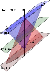
(a)

Figure 1: Cone I [blue] is bounded by a plane $b=-d+2$ and cone II [red] by a plane $b=-d+1$. Both cones are coaxial with axis described by the line $(\frac{1}{2},1,\frac{1}{2})+(1,-1,1)t$. Moreover, the special points are marked: associated with generalized Choi maps (i), (ii), (iv) and connected with reduction map (iii).

The above cones are described by the following equations: Cone I

$$(b-2)^{2}+(2c-3)^{2}+(d-2)^{2}+4bc+4cd-2bd=9\ ,$$ (34)

and Cone II

$$(b-1)^{2}+(2c-3)^{2}+(d-1)^{2}+4bc+4cd-2bd=6\ ,$$ (35)

with the constraints that $-b+1\leq d\leq-b+2$. The vertices of these cones are located at $b=\frac{1}{2},\ c=1,\ d=\frac{1}{2}$ and $b=1,\ c=\frac{1}{2},\ d=1$ for cones I and II, respectively. They intersect along an ellipse in the plane $d=-b+\frac{3}{2}$.

Let us analyze the intersection of the Cone I defined by (34) with the plane $b+d=2$. One finds

$$(d-1)^{2}+(c-\frac{1}{2})^{2}=\frac{1}{4}\ .$$ (36)

Similarly the intersection of the Cone II defined by (35) with the plane $b+d=1$ gives

$$(c-1)^{2}+(d-\frac{1}{2})^{2}=\frac{1}{4}\ .$$ (37)

Taking into account $a+b+c+d=3$ one finds

$$a = 1-c,$$

$$b = 1\pm\sqrt{c(1-c)},$$ (38)

$$d = 1\mp\sqrt{c(1-c)},$$

with $c\in[0,1]$ for the ellipse I on $b+d=2$ plane and

$$a = 1\pm\sqrt{d(1-d)},$$

$$b = 1-d,$$ (39)

$$c = 1\mp\sqrt{d(1-d)}$$

with $d\in[0,1]$ for the ellipse II on $b+d=1$ plane. Interestingly, ellipse I [blue] satisfies

$$a+c=1\ ,\ \ \ b+d=2\ ,$$ (40)

whereas the ellipse II [red] satisfies

$$a+c=2\ ,\ \ \ b+d=1\ .$$ (41)

Formulae (4) imply

$$bd=(1-a)^{2}\ .$$ (42)

Similarly, formulae (4) imply

$$ac=(1-b)^{2}\ .$$ (43)

These two equations provide an analog of the well known condition (18) for $n=3$.

Let us observe that these two ellipses contain already known positive maps:

• $\Phi[0,1,1,1]\,$ – reduction map [point (iii) in Fig. 1],

• $\Phi[1,1,1,0]\,$ – generalized Choi map [point (i) in Fig. 1],

• $\Phi[1,0,1,1]\,$ – generalized Choi map [point (ii) in Fig. 1],

• $\Phi[1,1,0,1]\,$ – [point (iv) in Fig. 1].

Note, however, that another generalized Choi map $\Phi[2,1,0,0]$ does not belong to our class.

5 (In)decomposability

In this section we analyze the issue of indecomposability of $\Phi[a,b,c,d]$.

Theorem 1

$\Phi[a,b,c,d]$ is decomposable if and only if $b=d$.

Proof: let us consider a state given by (unnormalized) density matrix

$$\rho_{\varepsilon}=\sum_{i=1}^{4}\Big{[}|ii\rangle\langle ii|+\varepsilon|i,i+1\rangle\langle i,i+1|+|i,i+2\rangle\langle i,i+2|+\varepsilon^{-1}|i,i+3\rangle\langle i,i+3|\Big{]}+\sum_{i\neq j}|ii\rangle\langle jj|\ ,$$ (44)

with $\varepsilon>0$. One easily checks that $\rho_{\varepsilon}$ is PPT. One finds

$$\mathrm{Tr}(W[a,b,c,d]\rho_{\varepsilon})=-12+4(a+c)+4\varepsilon^{-1}d+4\varepsilon b=4[d\varepsilon^{-1}+b\varepsilon-(b+d)]=4\varepsilon^{-1}[b\varepsilon^{2}-(b+d)\varepsilon+d]\ ,$$ (45)

and hence $\mathrm{Tr}(W[a,b,c,d]\rho_{\varepsilon})<0$ iff there exists $\varepsilon>0$ such that $b\varepsilon^{2}-(b+d)\varepsilon+d<0$. The corresponding discriminant reads

$$\Delta=(b+d)^{2}-4bd=(b-d)^{2}\ ,$$

and hence $b\varepsilon^{2}-(b+d)\varepsilon+d<0$ if $\varepsilon\in(\varepsilon_{-},\varepsilon_{+})$ with

$$\varepsilon_{\pm}=\frac{b+d\pm|b-d|}{2b}\ .$$

Note, that $\varepsilon_{+}>\varepsilon_{-}$ if and only if $b\neq d$. This way we have proved that if $b\neq d$ then $\Phi[a,b,c,d]$ is indecomposable. Now we show that if $b=d$, then $\Phi[a,b,c,d]$ is decomposable. We find the corresponding decomposition

$$W[a,b,c,d]=P[a,b,c,d]+Q[a,b,c,d]^{\Gamma},$$ (46)

where, $P[a,b,c,d]$ and $Q[a,b,c,d]$ are positive operators. One has

$$P[a,b,c,d]=\sum_{i=1}^{4}\Big{[}a|ii\rangle\langle ii|-(1-b)[\,|ii\rangle\langle i+1,i+1|+|ii\rangle\langle i+3,i+3|\,]-(1-c)|ii\rangle\langle i+2,i+2|\Big{]}\ ,$$ (47)

and

$$Q[a,b,c,d] = \sum_{i=1}^{4}\Big{[}b|i,i+1\rangle\langle i,i+1|+c|i,i+2\rangle\langle i,i+2|+b|i,i+3\rangle\langle i,i+3|$$ (48)

$$- b(\,|i,i+1\rangle\langle i+1,i|+|i,i+3\rangle\langle i+3,i|\,)-c|i,i+2\rangle\langle i+2,i|\Big{]}\ .$$

It is clear that $Q[a,b,c,d]\geq 0$. Now, to prove that $P[a,b,c,d]\geq 0$ one needs to show that the following circulant matrix

$$A=\left(\begin{array}[]{cccc}a&b-1&c-1&b-1\\ b-1&a&b-1&c-1\\ c-1&b-1&a&b-1\\ b-1&c-1&b-1&a\end{array}\right)\ ,$$ (49)

is positive. One finds for the eigenvalues of $A$: $\{0,4(1-b),2(2-b-c),2(2-b-c)\}$. Note, that $b+d\leq 2$ and hence $b=d\leq 1$. Moreover, $2-b-c=(a+c)-1\geq 0$. Hence $A\geq 0$.

$\Box$

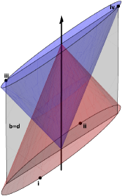
Figure 2: The intersection of the plane $b=d$ and of the blue and red cones represents decomposable EWs.

6 Structural Physical Approximation

For any entanglement witness $W$ in $\mathcal{H}_{A}\otimes\mathcal{H}_{B}$ such that ${\rm Tr}\,W=1$ one defines its structural physical approximation (SPA)

$$W(p)=(1-p)W+\frac{p}{d_{A}d_{B}}\mathbbm{1}_{A}\otimes\mathbbm{1}_{B},$$ (50)

with $p\geq p^{*}$, where $p^{*}$ is the smallest value of $p$ such that $W(p)\geq 0$. Thus, SPA defines a legitimate quantum state in $\mathcal{H}_{A}\otimes\mathcal{H}_{B}$. The conjecture of Korbicz et al. [20] (see also [21]) states that, if $W$ is an optimal EW, then its SPA defines separable state. It was supported by several examples (see e.g. [22]).

In a recent paper [14] it was conjectured that all entanglement witnesses $W[a,b,c]$ with $a,b,c$ satisfying (18) and $a\leq 1$ are optimal. Actually, this conjecture was proved by Ha and Kye [15] (see also [16]). It was shown [14] that $W[a,b,c]$ support SPA conjecture [20]. Now we prove the following

Proposition 1

If $a,b,c,d$ satisfy (4) or (4) then the structural physical approximation to $W[a,b,c,d]$ provides a separable state in $\mathbb{C}^{4}\otimes\mathbb{C}^{4}$.

Proof: Let us consider SPA for our class

$$\mathbf{W}(p)=(1-p)W+\frac{p}{16}\mathbb{I}_{4}\otimes\mathbb{I}_{4}\ .$$ (51)

Now, $\mathbf{W}(p)\geq 0$ for $p\geq p^{*}$, where the critical value $p^{*}$ is given by

$$p^{*}=\frac{4(a-3)}{3+4(a-3)}.$$ (52)

It turns out that $W(p^{*})$ can be represented as

$$\mathbf{W}(p^{*})=\frac{1}{4[3+4(a-3)]}(\sigma_{12}+\sigma_{13}+\sigma_{14}+\sigma_{23}+\sigma_{24}+\sigma_{34}+\sigma_{d}),$$ (53)

where

$$\sigma_{ij}=|ij\rangle\langle ij|+|ji\rangle\langle ji|+|ii\rangle\langle ii|+|jj\rangle\langle jj|-|ii\rangle\langle jj|-|jj\rangle\langle ii|,$$ (54)

and

$$\sigma_{d}=\sum_{i=1}^{4}\Big{(}(2b+c+d-1)|i,i+1\rangle\langle i,i+1|+(2c+b+d-1)|i,i+2\rangle\langle i,i+2|+(2d+b+c-1)|i,i+3\rangle\langle i,i+3|\Big{)}.$$ (55)

Due to the fact that $\sigma_{ij}$ are PPT and supported on $\mathbb{C}^{2}\otimes\mathbb{C}^{2}$, they are separable. Moreover, $\sigma_{d}$ is separable, whenever it defines a legitimate quantum state, that is, when

$$2b+c+d \geq 1,$$

$$2c+b+d \geq 1,$$ (56)

$$2d+b+c \geq 1.$$

It is straightforward to show that both conditions (4) and (4) imply (6) which ends the proof. $\Box$

Interestingly, the above three 2-dimensional planes:

$$2b+c+d=1\ ,\ \ 2c+b+d=1\ ,\ \ 2d+b+c=1\ ,$$

intersect at $b=c=d=1/4$.

7 Conclusions

We analyzed a class of positive maps in $M_{4}(\mathbb{C})$ (or equivalently class of EWs in $\mathcal{B}(\mathbb{C}^{4}\otimes\mathbb{C}^{4})$). This construction generalizes analysis provided in [14] for $n=3$ by replacing commutative group $SO(2)$ by the noncommutative rotation group $SO(3)$. We formulated necessary and sufficient conditions for positivity of $\Phi[a,b,c,d]$ and described the geometric structure of the convex set formed by these maps. Interestingly, there are two proper cones in the 3-dimensional space parameterized by $(b,c,d)$. It was shown that for $b\neq d$ all maps are indecomposable and hence can be used to detect PPT entangled states. Moreover, maps satisfying (6) support SPA conjecture [20]. We provided two natural 1-parameter subclasses of maps (cf. formulae (4) and (4)) – two ellipses in the parameter space – which are direct generalizations of 1-parameter class of maps analyzed in [14].

In a forthcoming paper we are going to analyze further properties of maps $\Phi[a,b,c,d]$. In particular optimality and atomicity. Finally, it would be interesting to provide the analogous construction for arbitrary $n$.

Appendix

$$a_{1}=\frac{3}{4}+\frac{1}{2}R_{11}+\frac{1}{2\sqrt{3}}R_{12}+\frac{1}{2\sqrt{6}}R_{13}+\frac{1}{2\sqrt{3}}R_{21}+\frac{1}{6}R_{22}+\frac{1}{6\sqrt{2}}R_{23}+\frac{1}{2\sqrt{6}}R_{31}+\frac{1}{6\sqrt{2}}R_{32}+\frac{1}{12}R_{33}\ ,$$

$$a_{2}=\frac{3}{4}-\frac{1}{2\sqrt{3}}R_{21}+\frac{1}{6}R_{22}+\frac{1}{6\sqrt{3}}R_{23}+\frac{1}{2}R_{11}-\frac{1}{2\sqrt{3}}R_{12}-\frac{1}{2\sqrt{6}}R_{13}-\frac{1}{2\sqrt{6}}R_{31}+\frac{1}{6\sqrt{2}}R_{32}+\frac{1}{12}R_{33}\ ,$$

$$a_{3}=\frac{3}{4}-\frac{1}{3\sqrt{2}}R_{32}+\frac{1}{12}R_{33}+\frac{2}{3}R_{22}-\frac{1}{3\sqrt{2}}R_{23}\ ,$$

$$a_{4}=\frac{3}{4}+\frac{9}{12}R_{33}\ ,$$

$$b_{1}=\frac{3}{4}-\frac{1}{2}R_{11}+\frac{1}{2\sqrt{3}}R_{12}+\frac{1}{2\sqrt{6}}R_{13}-\frac{1}{2\sqrt{3}}R_{21}+\frac{1}{6}R_{22}+\frac{1}{6\sqrt{2}}R_{23}-\frac{1}{2\sqrt{6}}R_{31}+\frac{1}{6\sqrt{2}}R_{32}+\frac{1}{12}R_{33}\ ,$$

$$b_{2}=\frac{3}{4}+\frac{1}{\sqrt{3}}R_{12}-\frac{1}{2\sqrt{6}}R_{13}-\frac{1}{3}R_{22}+\frac{1}{6\sqrt{2}}R_{23}-\frac{1}{3\sqrt{2}}R_{32}+\frac{1}{12}R_{33}\ ,$$

$$b_{3}=\frac{3}{4}-\frac{3}{12}R_{33}+\frac{1}{\sqrt{2}}R_{23}\ ,$$

$$b_{4}=\frac{3}{4}-\frac{3}{2\sqrt{6}}R_{31}-\frac{1}{2\sqrt{2}}R_{32}-\frac{3}{12}R_{33}\ ,$$

$$c_{1}=\frac{3}{4}-\frac{1}{\sqrt{3}}R_{12}+\frac{1}{2\sqrt{6}}R_{13}-\frac{1}{3}R_{22}+\frac{1}{6\sqrt{2}}R_{23}-\frac{1}{3\sqrt{2}}R_{32}+\frac{1}{12}R_{33}\ ,$$

$$c_{2}=\frac{3}{4}-\frac{1}{2\sqrt{2}}R_{23}+\frac{3}{2\sqrt{6}}R_{13}-\frac{3}{12}R_{33}\ ,$$

$$c_{3}=\frac{3}{4}+\frac{1}{2\sqrt{6}}R_{31}+\frac{1}{6\sqrt{2}}R_{32}+\frac{1}{12}R_{33}-\frac{1}{\sqrt{3}}R_{21}-\frac{1}{3}R_{22}-\frac{1}{3\sqrt{2}}R_{23}\ ,$$

$$c_{4}=\frac{3}{4}+\frac{3}{2\sqrt{6}}R_{31}-\frac{1}{2\sqrt{2}}R_{32}-\frac{3}{12}R_{33}\ ,$$

$$d_{1}=\frac{3}{4}-\frac{3}{2\sqrt{6}}R_{13}-\frac{1}{2\sqrt{2}}R_{23}-\frac{1}{4}R_{33}\ ,$$

$$d_{2}=\frac{3}{4}+\frac{1}{2\sqrt{3}}R_{21}+\frac{1}{6}R_{22}+\frac{1}{6\sqrt{2}}R_{23}-\frac{1}{2}R_{11}-\frac{1}{2\sqrt{3}}R_{12}-\frac{1}{2\sqrt{6}}R_{13}+\frac{1}{2\sqrt{6}}R_{31}+\frac{1}{6\sqrt{2}}R_{32}+\frac{1}{12}R_{33}\ ,$$

$$d_{3}=\frac{3}{4}-\frac{1}{2\sqrt{6}}R_{31}+\frac{1}{6\sqrt{2}}R_{32}+\frac{1}{12}R_{33}+\frac{1}{\sqrt{3}}R_{21}-\frac{1}{3}R_{22}-\frac{1}{3\sqrt{2}}R_{23}\ ,$$

$$d_{4}=\frac{3}{4}+\frac{1}{\sqrt{2}}R_{32}-\frac{3}{12}R_{33}\ .$$

References

• [1] R. Horodecki, P. Horodecki, M. Horodecki and K. Horodecki, Rev. Mod. Phys. 81, 865 (2009).
• [2] O. GΓΌhne and G. TΓ³th, Phys. Rep. 474, 1 (2009).
• [3] M. Horodecki, P. Horodecki, and R. Horodecki, Phys. Lett. A 223, 8 (1996).
• [4] B. M. Terhal, Phys. Lett. A 271, 319 (2000).
• [5] E. StΓΈrmer, in Lecture Notes in Physics 29, Springer Verlag, Berlin, 1974, pp. 85-106; Acta Math. 110, 233 (1963); Proc. Am. Math. Soc. 86, 402 (1982).
• [6] M.-D. Choi, Linear Alg. Appl. 12, 95 (1975); J. Operator Theory, 4, 271 (1980).
• [7] M.-D. Choi and T.-T. Lam, Math. Ann. 231, 1 (1977).
• [8] S. L. Woronowicz, Rep. Math. Phys. 10, 165 (1976); Comm. Math. Phys. 51, 243 (1976).
• [9] S. J. Cho, S.-H. Kye, and S. G. Lee, Linear Algebr. Appl. 171, 213 (1992).
• [10] A. Kossakowski, Open Sys. Inf. Dyn. 10, 1 (2003).
• [11] D. ChruΕ›ciΕ„ski and A. Kossakowski, Open Sys. Inf. Dyn. 14, 275 (2007).
• [12] D. ChruΕ›ciΕ„ski and A. Kossakowski, Phys. Lett. A 373 (2009) 2301-2305.
• [13] M. D. Choi, Linear Alg. Appl. 10, 285 (1975).
• [14] D. ChruΕ›ciΕ„ski and F. A. Wudarski, Open Syst. Inf. Dyn. 18, 387 (2011).
• [15] K-C. Ha and S-H. Kye, Phys. Rev. A 84, 024302 (2011).
• [16] D. ChruΕ›ciΕ„ski and G. Sarbicki, Optimal entanglement witnesses for two qutrits, arXiv:1105.4821.
• [17] K.-C. Ha and S.-H. Kye, Open Sys. Inf. Dyn. 18, 323 (2011).
• [18] S.-H. Kye, Facial structures for various notions of positivity and applications to the theory of entanglement, arXiv:1202.4255.
• [19] K. G. H. Vollbrecht and R. F. Werner, Phys. Rev. A 64, 062307 (2001).
• [20] J.K. Korbicz, M.L. Almeida, J. Bae, M. Lewenstein and A. Acin, Phys. Rev. A 78, 062105 (2008).
• [21] R. Augusiak, J. Bae, Ł. Czekaj, and M. Lewenstein, J. Phys. A: Math. Theor. 44, 185308 (2011).
• [22] D. ChruΕ›ciΕ„ski, J. Pytel and G. Sarbicki, Phys. Rev. A 80 (2009) 062314; D. ChruΕ›ciΕ„ski and J. Pytel, Phys. Rev. A 82 052310 (2010); D. ChruΕ›ciΕ„ski and J. Pytel, J. Phys. A: Math. Theor. 44, 165304 (2011).