Computation of the topological type of a real Riemann surface

Abstract.

We present an algorithm for the computation of the topological type of a real compact Riemann surface associated to an algebraic curve, i.e., its genus and the properties of the set of fixed points of the anti-holomorphic involution $\tau$, namely, the number of its connected components, and whether this set divides the surface into one or two connected components. This is achieved by transforming an arbitrary canonical homology basis to a homology basis where the $\mathcal{A}$-cycles are invariant under the anti-holomorphic involution $\tau$.

1. Introduction

Riemann surfaces have many applications in physics and mathematics as in topological field theories and in the theory of integrable partial differential equations (PDEs). In concrete applications such as solutions of PDEs, e.g. Korteweg-de Vries and nonlinear Schrödinger (NLS) equations, see e.g. [3] and references therein, physical quantities as for instance the amplitude of a water wave are real. Thus reality conditions on the solutions are important in practice. The corresponding solutions have to be constructed on real Riemann surfaces, i.e., surfaces with an anti-holomorphic involution $\tau$ acting as the complex conjugation on a local parameter on the surface. Regularity conditions for these solutions depend on the topological type of the surface, i.e., whether there are connected sets of fixed points of the involution $\tau$, the real ovals, and whether these ovals separate the surface into two connected components.

It is well known that all compact Riemann surfaces can be realized via nonsingular algebraic curves in $\mathbb{P}^{2}(\mathbb{C})$. F. Klein [28] observed that a real Riemann surface can be obtained in an analogous way from a nonsingular real plane algebraic curve $\mathcal{R}$ with an affine part of the form

(1.1) $$f(x,y)=\sum_{n=1}^{N}\sum_{m=1}^{M}a_{mn}x^{m}y^{n}=0,\qquad x,y\in\mathbb{C},\quad a_{mn}\in\mathbb{R}.$$

The focus of this paper is on real compact Riemann surfaces. For curves of the form (1.1) the action of the complex conjugation gives rise to an antiholomorphic involution $\tau$ defined on $\mathcal{R}$ by $\tau(x,y)=(\bar{x},\bar{y})$. The set of fixed points of $\tau$ is denoted by $\mathcal{R}(\mathbb{R})$ and is called the real part of $\mathcal{R}$. The connected components of $\mathcal{R}(\mathbb{R})$ are called real ovals. Historically, the first result in the topology of real algebraic curves was obtained by Harnack [21]: the number $k$ of real ovals of a curve $\mathcal{R}$ of genus $g$ satisfies $0\leq k\leq g+1$. In other words, the number of connected components of the real part of a real nonsingular plane algebraic curve cannot exceed $g+1$. Curves with the maximal number of real ovals are called M-curves.

The complement $\mathcal{R}\setminus\mathcal{R}(\mathbb{R})$ has either one or two connected components: if $\mathcal{R}\setminus\mathcal{R}(\mathbb{R})$ has two components, the curve $\mathcal{R}$ is called a dividing curve, otherwise it is called non-dividing (notice that an M-curve is always a dividing curve). The topological type of $\mathcal{R}$ is usually denoted by $(g,k,a)$ where $g$ denotes the genus, $k$ the number of real ovals, and $a=0$ if the curve is dividing, $a=1$ if it is non-dividing. This implies that the topological type of a curve without real oval is $(g,0,1)$. Notice that the first part of Hilbert’s 16th problem is concerned with the relative configuration of real ovals of a plane algebraic curve of given degree in $\mathbb{P}^{2}(\mathbb{R})$, i.e., how many ovals can lie in interior of another oval. This question has been studied by many authors, see, for instance, [23, 32, 31, 20, 39, 1] and references therein. However, until now the complete answer is known only for curves of degree 7 and less. We will not discuss this topic here, but we would like to mention that in general, a solution to this problem, namely, the knowledge of the embedding $\mathcal{R}(\mathbb{R})\subset\mathbb{P}^{2}(\mathbb{R})$, does not provide any information on the embedding $\mathcal{R}(\mathbb{R})\subset\mathcal{R}$ which is the subject of the present paper. For instance, it is possible to construct two real plane algebraic curves having the same degree and the same configuration of ovals, one of them being dividing and the other non-dividing (see [18] p. 8).

The aim of this paper is twofold: to determine the topological type $(g,k,a)$ of a real algebraic curve of the form (1.1) with a numerical approach, and to transform periods of the holomorphic differentials of the curve to a form where the $\mathcal{A}$-periods are real. There exist various algorithms which give the oval arrangements of a given real algebraic curve, see, for instance, [2, 8, 33, 14, 19, 25, 34], all of them following the same scheme. But to the best of our knowledge, there exists no algorithm that computes the parameter $a$ in the topological type $(g,k,a)$ of $\mathcal{R}$, which encodes the property of the curve to be dividing or not. The starting point of our algorithm is the work by Deconinck and van Hoeij who developed an approach to the symbolic-numerical treatment of algebraic curves. This approach is distributed as the algcurves package with Maple, see [9, 10, 11]. A purely numerical approach to real hyperelliptic Riemann surfaces was given in [15, 16], and for general Riemann surfaces in [17]. For a review on computational approaches to Riemann surfaces the reader is referred to [4].

The codes [11, 17] compute the periods of a Riemann surface in a homology basis which is determined by an algorithm due to Tretkoff and Tretkoff [36]. This homology basis is in general not adapted to possible symmetries of the curve (as the involution $\tau$ of real curves). It means that the action on the computed homology basis of any automorphism of the curve cannot be expressed in a simple way in terms of this basis. However, the choice of a basis, where certain cycles are invariant under the automorphisms, is often convenient in applications. In the context of solutions to integrable PDEs on general compact Riemann surfaces as for the Kadomtsev-Petviashvili (KP) (see [13]) and the Davey-Stewartson (DS) equations (see [30, 26]), smoothness conditions are formulated conveniently in a homology basis adapted to the anti-holomorphic involution $\tau$ defined on the surface. For instance, on a real surface there exists a canonical homology basis $(\mathcal{A},\mathcal{B})$ (that we call for simplicity symmetric homology basis in the following) satisfying the conditions (see [35, 38])

$$\left(\begin{matrix}\tau\mathbf{\mathcal{A}}\\ \tau\mathbf{\mathcal{B}}\end{matrix}\right)=\left(\begin{matrix}\mathbb{I}_{g}&\,\,0\\ \mathbb{H}\,\,&-\mathbb{I}_{g}\end{matrix}\right)\left(\begin{matrix}\mathbf{\mathcal{A}}\\ \mathbf{\mathcal{B}}\end{matrix}\right),$$

where $\mathbb{H}\in\mathcal{M}_{g}(\mathbb{Z}/2\mathbb{Z})$ is a $g\times g$ matrix which depends on the topological type $(g,k,a)$ (see section 2); here $\mathbb{I}_{g}$ denotes the $g\times g$ unit matrix.

In [27] we studied for the first time numerically solutions to integrable equations from the family of NLS equations, namely, the multi-component nonlinear Schr dinger equation and the $(2+1)$-dimensional DS equations. A symplectic transformation of the computed homology basis to the symmetric homology basis was introduced in [27] and was constructed explicitly for concrete examples. In the present work we give in Theorem 3.24 a complete description of such a symplectic transformation depending on the topological type of the underlying real algebraic curve. The formulas are expressed in terms of period matrices of holomorphic differentials on the curve; these holomorphic differentials must satisfy the condition $\overline{\tau^{*}\nu_{j}}=\nu_{j}$, $j=1,\ldots,g$, where $\tau^{*}$ is the action of $\tau$ lifted to the space of holomorphic differentials. This allows to give an algorithm to construct explicitly a symplectic transformation of an arbitrary canonical homology basis for a real Riemann surface to the symmetric form. The algorithm permits to systematically study smooth real solutions on general real Riemann surfaces for equations like KP and DS starting from a representation of the surface via an algebraic curve which so far was only possible for hyperelliptic surfaces. In addition, this provides a numerical way to compute the topological type of a real Riemann surface for given periods of the holomorphic differentials.

The paper is organized as follows. In section 2 we introduce a symmetric homology basis which depends on the topological type of $\mathcal{R}$. In section 3 we give explicitly the symplectic transformation between the computed homology basis and the symmetric homology basis. This result will be used in section 4 to construct an algorithm which gives the topological type $(g,k,a)$ of a real algebraic curve for given periods of the holomorphic differentials. In section 5 we discuss examples of real curves for higher genus. Some concluding remarks are added in section 6.

2. Symmetric homology basis

In what follows $\mathcal{R}$ denotes a compact Riemann surface of genus $g>0$. A homology basis $(\mathcal{A},\mathcal{B}):=(\mathcal{A}_{1},\ldots,\mathcal{A}_{g},\mathcal{B}_{1},\ldots,\mathcal{B}_{g})$ with the following intersection indices

$$\mathcal{A}_{i}\circ\mathcal{B}_{j}=\delta_{ij}\qquad\quad\mathcal{A}_{i}\circ\mathcal{A}_{j}=\mathcal{B}_{i}\circ\mathcal{B}_{j}=0,$$

is called a canonical basis of cycles. With $\mathcal{A}$ (resp. $\mathcal{B}$) we denote the vector $(\mathcal{A}_{1},\ldots,\mathcal{A}_{g})^{t}$ (resp. $(\mathcal{B}_{1},\ldots,\mathcal{B}_{g})^{t}$). Canonical homology bases are related via a symplectic transformation. Let $(\mathbf{\mathcal{A}},\mathbf{\mathcal{B}})$ and $(\mathbf{\tilde{\mathcal{A}}},\mathbf{\tilde{\mathcal{B}}})$ be arbitrary canonical homology bases on $\mathcal{R}$. Then there exists a symplectic matrix $\left(\begin{matrix}A&B\\ C&D\end{matrix}\right)\in Sp(2g,\mathbb{Z})$ such that

(2.1) $$\left(\begin{matrix}A&B\\ C&D\end{matrix}\right)\left(\begin{matrix}\mathbf{\tilde{\mathcal{A}}}\\ \mathbf{\tilde{\mathcal{B}}}\end{matrix}\right)=\left(\begin{matrix}\mathbf{\mathcal{A}}\\ \mathbf{\mathcal{B}}\end{matrix}\right).$$

Recall that a symplectic matrix $M\in Sp(2g,\mathbb{Z})$ satisfies $M^{t}J_{g}M=J_{g}$, with the matrix $J_{g}$ given by $J_{g}=\left(\begin{matrix}0&\,\,\mathbb{I}_{g}\\ -\mathbb{I}_{g}\,\,&0\end{matrix}\right),$ where $\mathbb{I}_{g}$ denotes the $g\times g$ unit matrix. Symplectic matrices $M=\left(\begin{matrix}A&B\\ C&D\end{matrix}\right)\in Sp(2g,\mathbb{Z})$ are characterized by the following system:

(2.2) $$A^{t}D- C^{t}B=\mathbb{I}_{g},$$

(2.3) $$A^{t}C =C^{t}A,$$

(2.4) $$D^{t}B =B^{t}D.$$

Moreover, the inverse matrix $M^{-1}$ is given by

(2.5) $$M^{-1}=\left(\begin{matrix}\,\,\,\,D^{t}&-B^{t}\,\\ -C^{t}&\,\,\,A^{t}\end{matrix}\right).$$

Now let $\tau$ be an anti-holomorphic involution defined on $\mathcal{R}$. Recall that $(g,k,a)$ denotes the topological type of $\mathcal{R}$, where $k$ is the number of connected components of $\mathcal{R}(\mathbb{R})$ (the set of fixed points of $\tau$), and $a=0$ if the curve is dividing (i.e., if $\mathcal{R}\setminus\mathcal{R}(\mathbb{R})$ has two components), $a=1$ if it is non-dividing (i.e., if $\mathcal{R}\setminus\mathcal{R}(\mathbb{R})$ has just one component). A curve with the topological type $(g,g+1,0)$ is called an M-curve. According to Proposition 2.2 in Vinnikov’s paper [38], there exists a canonical homology basis $(\mathcal{A},\mathcal{B})$ (called for simplicity symmetric homology basis) such that

(2.6) $$\left(\begin{matrix}\tau\mathbf{\mathcal{A}}\\ \tau\mathbf{\mathcal{B}}\end{matrix}\right)=\left(\begin{matrix}\mathbb{I}_{g}&\,\,0\\ \mathbb{H}\,\,&-\mathbb{I}_{g}\end{matrix}\right)\left(\begin{matrix}\mathbf{\mathcal{A}}\\ \mathbf{\mathcal{B}}\end{matrix}\right),$$

where $\mathbb{H}$ is a block diagonal $g\times g$ matrix which depends on the topological type $(g,k,a)$ of $\mathcal{R}$ and is defined as follows:

- if $k>0$ and $a=0$,

$$\mathbb{H}={\left(\begin{matrix}0&1&&&&&&\\ 1&0&&&&&&\\ &&\ddots&&&&&\\ &&&0&1&&&\\ &&&1&0&&&\\ &&&&&0&&\\ &&&&&&\ddots&\\ &&&&&&&0\end{matrix}\right)},$$

- if $k>0$ and $a=1$,

$$\mathbb{H}={\left(\begin{matrix}1&&&&&\\ &\ddots&&&&\\ &&1&&&\\ &&&0&&\\ &&&&\ddots&\\ &&&&&0\end{matrix}\right)};$$

rank$(\mathbb{H})=g+1-k$ in both cases;

- if $k=0$,

$$\mathbb{H}={\left(\begin{matrix}0&1&&&\\ 1&0&&&\\ &&\ddots&&\\ &&&0&1\\ &&&1&0\end{matrix}\right)}\quad\text{for even $g$ or}\quad\mathbb{H}={\left(\begin{matrix}0&1&&&&\\ 1&0&&&&\\ &&\ddots&&&\\ &&&0&1&\\ &&&1&0&\\ &&&&&0\end{matrix}\right)}\mbox{ for odd $g$};$$

rank$(\mathbb{H})=g$ if $g$ is even, rank$(\mathbb{H})=g-1$ if $g$ is odd.

Remark 2.1.

For given information whether there are real ovals ($k>0$) or not ($k=0$), the matrix $\mathbb{H}$ completely encodes the topological type of the real Riemann surface. In [35] a different, but equivalent form of $\mathbb{H}$ was used, which has ones only in the antidiagonal, if the rank is equal to the genus, or in a parallel to the antidiagonal for smaller rank.

Example 2.1.

Consider the hyperelliptic curve of genus $g$ defined by the equation

(2.7) $$y^{2}=\prod_{i=1}^{2g+2}(x-x_{i}),$$

where the branch points $x_{i}\in\mathbb{R}$ are ordered such that $x_{1}<\ldots<x_{2g+2}$. On such a curve, we can define two anti-holomorphic involutions $\tau_{1}$ and $\tau_{2}$, given respectively by $\tau_{1}(x,y)=(\overline{x},\overline{y})$ and $\tau_{2}(x,y)=(\overline{x},-\overline{y})$. Projections of real ovals of $\tau_{1}$ on the $x$-plane coincide with the intervals $[x_{2g+2},x_{1}],\ldots,[x_{2g},x_{2g+1}]$, whereas projections of real ovals of $\tau_{2}$ on the $x$-plane coincide with the intervals $[x_{1},x_{2}],\ldots,[x_{2g+1},x_{2g+2}]$. Hence the curve (2.7) is an M-curve with respect to both anti-involutions $\tau_{1}$ and $\tau_{2}$.

If all $x_{i}$ are non-real and pairwise conjugate, the curve has no real ovals with respect to the involution $\tau_{2}$; it is dividing for the involution $\tau_{1}$.

3. Symplectic transformation between homology bases

In this section we construct a symplectic transformation between an arbitrary homology basis $(\mathcal{\tilde{A}},\mathcal{\tilde{B}})$ and a symmetric homology basis on a real Riemann surface $(\mathcal{R},\tau)$, where $\tau$ denotes the anti-holomorphic involution defined on $\mathcal{R}$. The main result of this paper is contained in Theorem 3.24 which gives the underlying symplectic matrix $\left(\begin{matrix}A&B\\ C&D\end{matrix}\right)$ in terms of the period matrices of holomorphic differentials satisfying the condition (3.2) in the homology basis $(\mathcal{\tilde{A}},\mathcal{\tilde{B}})$. The key ingredient in this context is the description of the action of $\tau$ on the cycles $(\mathcal{\tilde{A}},\mathcal{\tilde{B}})$, given in Proposition 3.17 by the integer matrix $\mathbf{R}$. Then Theorem 3.24 states that the column vectors of the matrix $\left(\begin{matrix}A&B\end{matrix}\right)^{t}$ form in fact a $\mathbb{Z}$-basis of the integer kernel of the matrix $\mathbf{R}^{t}-\mathbb{I}_{2g}$. The matrix $Q$ in Theorem 3.24 encodes the degree of freedom in the choice of such a $\mathbb{Z}$-basis. For the ease of the reader, we start recalling some basic facts from the theory of $\mathbb{Z}$-modules used to prove Theorem 3.24, which differs from the usual linear algebra over vector spaces.

3.1. Basic facts from the theory of $\mathbb{Z}$-modules

A $\mathbb{Z}$-module or more generally a $\mathbb{A}$-module where $\mathbb{A}$ denotes a commutative ring, is a natural generalization of vector spaces where the usual scalar field is replaced by the ring $\mathbb{A}$. For a review on the subject we refer to [29]. In what follows we assume that $\mathbb{A}$ is the principal ring $\mathbb{Z}$ and we denote by $\mathcal{M}$ a $\mathbb{Z}$-module.

Definition 3.1.

2. $\mathcal{M}$ is of finite type if it admits a finite set of generators.

3. $\mathcal{M}$ is said to be free if there exists a $\mathbb{Z}$-basis, namely, a set $\{x_{i}\}_{i\in I}\subset\mathcal{M}$ with $I\subset\mathbb{N}$ such that any element $x\in\mathcal{M}$ can be written uniquely as $x=\sum_{i\in I}\alpha_{i}\,x_{i}$ where the scalars $\alpha_{i}\in\mathbb{Z}$ are non-zero only for a finite number of them.

The following theorems provide important results in the general theory of modules over a principal ring.

Theorem 3.1.

2. If $\mathcal{M}$ is free and of finite type then all $\mathbb{Z}$-bases of $\mathcal{M}$ are finite with the same cardinality called the $rank$ of $\mathcal{M}$.

3. Since $\mathbb{Z}$ is integral, the rank of $\mathcal{M}$ equals the dimension of the $\mathbb{Q}$-vector space $\mathbb{S}^{-1}\mathcal{M}$ where $\mathbb{S}=\mathbb{Z}\setminus\{0\}$.

4. A submodule of a free $\mathbb{Z}$-module of finite type of rank $n$ is a free $\mathbb{Z}$-module of finite type of rank $r\leq n$.

The example we will need in this paper are submodules of $\mathbb{Z}^{n}$ which are because of the Theorem 3.1 free modules of finite type with rank $r\leq n$.

Remark 3.1.

Contrary to the case of vector spaces, if $\mathcal{N}$ is a free submodule of the free module $\mathcal{M}$ with the same rank, this does not imply that $\mathcal{N}$ equals $\mathcal{M}$. Consider the submodule $2\mathbb{Z}$ of $\mathbb{Z}$ as an example.

The following theorem, also called the theorem of the adapted basis, gives the classification of modules over the principal ring $\mathbb{Z}$:

Theorem 3.2.

Let $\mathcal{M}$ be a free $\mathbb{Z}$-module of rank $n$ and let $\mathcal{N}$ be a submodule of $\mathcal{M}$. Then there exists a basis $(e_{1},\ldots,e_{n})$ of $\mathcal{M}$ and unique non-zero integers $(p_{1},\ldots,p_{r})$ (with $r\leq n$) such that

1. $(p_{1}e_{1},\ldots,p_{r}e_{r})$ is a $\mathbb{Z}$-basis of $\mathcal{N}$

2. $p_{1}|p_{2}|\ldots|p_{r}$ (this means that $\forall i$, $p_{i}$ divides all $p_{j}$ with $j>i$).

In what follows $GL_{n}(\mathbb{Z})$ denotes the set of $n\times n$ invertible matrices over $\mathbb{Z}$; it is well known that the determinant of these matrices equals $\pm 1$. Notice that if $M$ denotes the matrix formed by the column vectors of a $\mathbb{Z}$-basis of a $\mathbb{Z}$-module of rank $n$, then other bases are given by the column vectors of matrices of the form $MQ$ with $Q\in GL_{n}(\mathbb{Z})$. Therefore, Theorem 3.2 has the following matrix interpretation that we will use in section 3.3: for any non-zero $m\times n$ matrix $M\in\mathcal{M}_{m,n}(\mathbb{Z})$ of rank $r$, there exist matrices $U\in GL_{m}(\mathbb{Z})$, $V\in GL_{n}(\mathbb{Z})$ such that

(3.1) $$UMV=\left(\begin{matrix}\text{Diag}(p_{1},\ldots,p_{r})&0\\ 0&0\end{matrix}\right),$$

where $p_{i}\in\mathbb{Z}\setminus\{0\}$ satisfy $p_{1}|p_{2}|\ldots|p_{r}$ and where $\text{Diag}(.)$ denotes the diagonal matrix. This is called the Smith normal form of $M$. In section 4 we will use a well known algorithm to compute the Smith normal form. In particular, this algorithm provides a $\mathbb{Z}$-basis of the integer kernel of $M$ given by the last $n-r$ column vectors of the matrix $V$ in (3.1).

3.2. Action of $\tau$ on an arbitrary homology basis

We denote by $(\mathbf{\mathcal{A}},\mathbf{\mathcal{B}})$ a symmetric homology basis (i.e. which satisfies (2.6)). Let $(\nu_{1},\ldots,\nu_{g})$ be a basis of holomorphic differentials such that

(3.2) $$\overline{\tau^{*}\nu_{j}}=\nu_{j},\qquad j=1,\ldots,g,$$

where $\tau^{*}$ is the action of $\tau$ lifted to the space of holomorphic differentials: $\tau^{*}\omega(p)=\omega(\tau p)$ for any $p\in\mathcal{R}$. The matrices $P_{\mathcal{A}}$ and $P_{\mathcal{B}}$ defined by

(3.3) $$(P_{\mathcal{A}})_{ij}=\int_{\mathcal{A}_{i}}\nu_{j},\qquad(P_{\mathcal{B}})_{ij}=\int_{\mathcal{B}_{i}}\nu_{j},\qquad i,j=1,\ldots,g$$

are called the matrices of $\mathcal{A}$- and $\mathcal{B}$-periods of the differentials $\nu_{j}$. From (2.6) and (3.2) we deduce the action of the complex conjugation on the matrices $P_{\mathcal{A}}$ and $P_{\mathcal{B}}$:

(3.4) $$(P_{\mathcal{A}})_{ij}\in\mathbb{R},$$

(3.5) $$\overline{P_{\mathcal{B}}}=-P_{\mathcal{B}}+\mathbb{H}P_{\mathcal{A}}.$$

Denote by $(\mathbf{\tilde{\mathcal{A}}},\mathbf{\tilde{\mathcal{B}}})$ an arbitrary homology basis. From the symplectic transformation (2.1) we obtain the following transformation law between the matrices $P_{\tilde{\mathcal{A}}},P_{\tilde{\mathcal{B}}}$ and $P_{\mathcal{A}},P_{\mathcal{B}}$ defined in (3.3):

(3.6) $$\left(\begin{matrix}A&B\\ C&D\end{matrix}\right)\left(\begin{matrix}P_{\tilde{\mathcal{A}}}\\ P_{\tilde{\mathcal{B}}}\end{matrix}\right)=\left(\begin{matrix}P_{\mathcal{A}}\\ P_{\mathcal{B}}\end{matrix}\right).$$

Therefore, by (3.4) one gets

(3.7) $$A\,\text{Re}\left(P_{\tilde{\mathcal{A}}}\right)+B\,\text{Re}\left(P_{\tilde{\mathcal{B}}}\right) =P_{\mathcal{A}}$$

(3.8) $$A\,\text{Im}\left(P_{\tilde{\mathcal{A}}}\right)+B\,\text{Im}\left(P_{\tilde{\mathcal{B}}}\right) =0,$$

and by (3.5)

(3.9) $$C\,\text{Re}\left(P_{\tilde{\mathcal{A}}}\right)+D\,\text{Re}\left(P_{\tilde{\mathcal{B}}}\right) =\frac{1}{2}\,\mathbb{H}P_{\mathcal{A}}$$

(3.10) $$C\,\text{Im}\left(P_{\tilde{\mathcal{A}}}\right)+D\,\text{Im}\left(P_{\tilde{\mathcal{B}}}\right) =\text{Im}\left(P_{\mathcal{B}}\right).$$

From (3.7) and (3.10) it can be checked that the matrices $A\,\text{Re}\left(P_{\tilde{\mathcal{A}}}\right)+B\,\text{Re}\left(P_{\tilde{\mathcal{B}}}\right)$ and $C\,\text{Im}\left(P_{\tilde{\mathcal{A}}}\right)+D\,\text{Im}\left(P_{\tilde{\mathcal{B}}}\right)$ are invertible (the first because $P_{\mathcal{A}}$ is, for the second see [27] for more details). The following Lemma proved in [27] shows that it is sufficient to know the pairs of matrices $A,B$ or $C,D$ to get the full symplectic transformation (3.6):

Lemma 3.1.

The matrices $A,B,C,D\in\mathcal{M}_{g}(\mathbb{Z})$ solving (3.7)-(3.10) satisfy:

(3.11) $$A^{t} =\text{Im}\left(P_{\tilde{\mathcal{B}}}\right)\left[C\,\text{Im}\left(P_{\tilde{\mathcal{A}}}\right)+D\,\text{Im}\left(P_{\tilde{\mathcal{B}}}\right)\right]^{-1}$$

(3.12) $$B^{t} =-\text{Im}\left(P_{\tilde{\mathcal{A}}}\right)\left[C\,\text{Im}\left(P_{\tilde{\mathcal{A}}}\right)+D\,\text{Im}\left(P_{\tilde{\mathcal{B}}}\right)\right]^{-1}$$

(3.13) $$C^{t} =\frac{1}{2}\,A^{t}\mathbb{H}-\text{Re}\left(P_{\tilde{\mathcal{B}}}\right)\left[A\,\text{Re}\left(P_{\tilde{\mathcal{A}}}\right)+B\,\text{Re}\left(P_{\tilde{\mathcal{B}}}\right)\right]^{-1}$$

(3.14) $$D^{t} =\frac{1}{2}\,B^{t}\mathbb{H}+\text{Re}\left(P_{\tilde{\mathcal{A}}}\right)\left[A\,\text{Re}\left(P_{\tilde{\mathcal{A}}}\right)+B\,\text{Re}\left(P_{\tilde{\mathcal{B}}}\right)\right]^{-1}.$$

The action of $\tau$ on an arbitrary homology basis $(\mathbf{\tilde{\mathcal{A}}},\mathbf{\tilde{\mathcal{B}}})$ can be written as

(3.15) $$\left(\begin{matrix}\tau\mathbf{\tilde{\mathcal{A}}}\\ \tau\mathbf{\tilde{\mathcal{B}}}\end{matrix}\right)=\mathbf{R}\left(\begin{matrix}\mathbf{\tilde{\mathcal{A}}}\\ \mathbf{\tilde{\mathcal{B}}}\end{matrix}\right),$$

where $\mathbf{R}\in\mathcal{M}_{2g}(\mathbb{Z})$. In the following proposition, we give an explicit expression for the matrix $\mathbf{R}$ in terms of the period matrices $P_{\tilde{\mathcal{A}}}$ and $P_{\tilde{\mathcal{B}}}$ only.

Proposition 3.1.

The matrix $\mathbf{R}$ defined in (3.15) is given by

(3.16) $$\mathbf{R}=\left(\begin{matrix}\left(2\,\text{Re}\left(P_{\tilde{\mathcal{B}}}\right)\tilde{\mathbb{M}}^{-1}\,\text{Im}\left(P_{\tilde{\mathcal{A}}}^{t}\right)+\mathbb{I}_{g}\right)^{t}&-2\,\text{Re}\left(P_{\tilde{\mathcal{A}}}\right)\tilde{\mathbb{M}}^{-1}\,\text{Im}\left(P_{\tilde{\mathcal{A}}}^{t}\right)\\ 2\,\text{Re}\left(P_{\tilde{\mathcal{B}}}\right)\tilde{\mathbb{M}}^{-1}\,\text{Im}\left(P_{\tilde{\mathcal{B}}}^{t}\right)&-\left(2\,\text{Re}\left(P_{\tilde{\mathcal{B}}}\right)\tilde{\mathbb{M}}^{-1}\,\text{Im}\left(P_{\tilde{\mathcal{A}}}^{t}\right)+\mathbb{I}_{g}\right)\end{matrix}\right),$$

where

(3.17) $$\tilde{\mathbb{M}}=\text{Im}\left(P_{\tilde{\mathcal{B}}}^{t}\right)\text{Re}\left(P_{\tilde{\mathcal{A}}}\right)-\text{Im}\left(P_{\tilde{\mathcal{A}}}^{t}\right)\text{Re}\left(P_{\tilde{\mathcal{B}}}\right).$$

Proof.

Using (2.6) we deduce the action of $\tau$ on (2.1):

(3.18) $$\left(\begin{matrix}A&B\\ C&D\end{matrix}\right)^{-1}\left(\begin{matrix}\mathbb{I}_{g}&\,\,0\\ \mathbb{H}\,\,&-\mathbb{I}_{g}\end{matrix}\right)\left(\begin{matrix}\mathbf{\mathcal{A}}\\ \mathbf{\mathcal{B}}\end{matrix}\right)=\mathbf{R}\left(\begin{matrix}A&B\\ C&D\end{matrix}\right)^{-1}\left(\begin{matrix}\mathbf{\mathcal{A}}\\ \mathbf{\mathcal{B}}\end{matrix}\right),$$

which yields

(3.19) $$\mathbf{R}=\left(\begin{matrix}A&B\\ C&D\end{matrix}\right)^{-1}\left(\begin{matrix}\mathbb{I}_{g}&\,\,0\\ \mathbb{H}\,\,&-\mathbb{I}_{g}\end{matrix}\right)\left(\begin{matrix}A&B\\ C&D\end{matrix}\right).$$

In other words, a symplectic matrix which transforms a basis $(\tilde{\mathcal{A}},\tilde{\mathcal{B}})$ to a symmetric form also satisfies (3.19). From (3.19) and (2.5) one gets

(3.20) $$\mathbf{R}=\left(\begin{matrix}(2\,C^{t}B-A^{t}\mathbb{H}B+\mathbb{I}_{g})^{t}&2\,D^{t}B-B^{t}\mathbb{H}B\\ -2\,C^{t}A+A^{t}\mathbb{H}A&-(2\,C^{t}B-A^{t}\mathbb{H}B+\mathbb{I}_{g})\end{matrix}\right).$$

Replacing $A$ via (3.11) and $B$ via (3.12) in (3.13) and then using (3.11) again to eliminate the factor $\left[C\,\text{Im}\left(P_{\tilde{\mathcal{A}}}\right)+D\,\text{Im}\left(P_{\tilde{\mathcal{B}}}\right)\right]$ leads to a relation for $C^{t}A$ only (using in the last step (3.12) instead of (3.11) gives a relation for $C^{t}B$). Similarly one gets a relation for $D^{t}B$,

$$2\,C^{t}A =A^{t}\mathbb{H}A-2\,\text{Re}\left(P_{\tilde{\mathcal{B}}}\right)\tilde{\mathbb{M}}^{-1}\,\text{Im}\left(P_{\tilde{\mathcal{B}}}^{t}\right),$$

$$2\,C^{t}B =A^{t}\mathbb{H}B+2\,\text{Re}\left(P_{\tilde{\mathcal{B}}}\right)\tilde{\mathbb{M}}^{-1}\,\text{Im}\left(P_{\tilde{\mathcal{A}}}^{t}\right),$$

$$2\,D^{t}B =B^{t}\mathbb{H}B-2\,\text{Re}\left(P_{\tilde{\mathcal{A}}}\right)\tilde{\mathbb{M}}^{-1}\,\text{Im}\left(P_{\tilde{\mathcal{A}}}^{t}\right),$$

with $\tilde{\mathbb{M}}$ given by (3.17). Substituting these relations in (3.20) one gets (3.16). ∎

3.3. Symplectic transformation

In this part we present in Theorem 3.24 the main result of the present paper: the symplectic transformation between an arbitrary basis $(\tilde{\mathcal{A}},\tilde{\mathcal{B}})$ on a real Riemann surface and a homology basis adapted to the symmetry is given in terms of the period matrices $P_{\tilde{\mathcal{A}}},P_{\tilde{\mathcal{B}}}$ defined in the previous section. This result will allow to construct in section 4 an algorithm which computes the topological type of a given real Riemann surface.

We start with the following lemma which describes the spectral properties of the matrix $\mathbf{R}$ (3.16):

Lemma 3.2.

The matrix $\mathbf{R}$ in (3.16) is diagonalizable over $\mathbb{Q}$ with eigenvalues $1$ and $-1$. The dimension of the corresponding eigenspaces equals $g$.

Proof.

It is straightforward to see that the matrix $\left(\begin{matrix}\mathbb{I}_{g}&\,\,0\\ \mathbb{H}\,\,&-\mathbb{I}_{g}\end{matrix}\right)$ is diagonalizable over $\mathbb{Q}$: the eigenvalues are $1$ and $-1$, and the dimension of the corresponding eigenspaces equals $g$. Therefore, by (3.19) the same holds for the matrix $\mathbf{R}$. ∎

In what follows we denote by

(3.21) $$\mathcal{K}_{\mathbb{Z}}:=\left\{w\in\mathbb{Z}^{2g};(\mathbf{R}^{t}-\mathbb{I}_{2g})w=0\right\}$$

the integer kernel of the matrix $\mathbf{R}^{t}-\mathbb{I}_{2g}$. According to the theory of modules over the principal ring $\mathbb{Z}$, the $\mathbb{Z}$-module $\mathcal{K}_{\mathbb{Z}}$ admits a $\mathbb{Z}$-basis which can, for instance, be computed from the Smith normal form (see section 3.1).

Theorem 3.3.

Let $\mathcal{R}$ be a real compact Riemann surface of genus $g$ and $(\mathbf{\tilde{\mathcal{A}}},\mathbf{\tilde{\mathcal{B}}})$ a canonical homology basis on $\mathcal{R}$. For the given matrices of periods $P_{\tilde{\mathcal{A}}},P_{\tilde{\mathcal{B}}}$ of holomorphic differentials satisfying (3.2), let $\left(\begin{matrix}S_{1}\\ S_{2}\end{matrix}\right)$ be the $2g\times g$ matrix formed by a $\mathbb{Z}$-basis of $\mathcal{K}_{\mathbb{Z}}$ (3.21). Then a symplectic matrix in (2.1) which relates the homology basis $(\mathbf{\tilde{\mathcal{A}}},\mathbf{\tilde{\mathcal{B}}})$ to a symmetric homology basis $(\mathbf{\mathcal{A}},\mathbf{\mathcal{B}})$ is given by:

(3.22) $$\left(\begin{matrix}A^{t}\\ B^{t}\end{matrix}\right) =\left(\begin{matrix}S_{1}\\ S_{2}\end{matrix}\right)Q$$

(3.23) $$\left(\begin{matrix}C^{t}\\ D^{t}\end{matrix}\right) =\frac{1}{2}\left(\begin{matrix}S_{1}\\ S_{2}\end{matrix}\right)Q\mathbb{H}+\left(\begin{matrix}-\text{Re}\left(P_{\tilde{\mathcal{B}}}\right)\\ \,\,\,\,\text{Re}\left(P_{\tilde{\mathcal{A}}}\right)\end{matrix}\right)\left[S_{1}^{t}\,\text{Re}\left(P_{\tilde{\mathcal{A}}}\right)+S_{2}^{t}\,\text{Re}\left(P_{\tilde{\mathcal{B}}}\right)\right]^{-1}(Q^{t})^{-1}$$

where the matrix $\mathbb{H}$ is defined in section 2, and where $Q\in GL_{g}(\mathbb{Z})$ is such that

(3.24) $$\left(\begin{matrix}S_{1}\\ S_{2}\end{matrix}\right)Q\mathbb{H}Q^{t}\equiv 2\left(\begin{matrix}-\text{Re}\left(P_{\tilde{\mathcal{B}}}\right)\\ \,\,\,\,\text{Re}\left(P_{\tilde{\mathcal{A}}}\right)\end{matrix}\right)\left[S_{1}^{t}\,\text{Re}\left(P_{\tilde{\mathcal{A}}}\right)+S_{2}^{t}\,\text{Re}\left(P_{\tilde{\mathcal{B}}}\right)\right]^{-1}\quad(\text{mod}\,\,2).$$

Proof.

Notice that (3.19) can be rewritten as

(3.25) $$\left(\begin{matrix}A&B\\ C&D\end{matrix}\right)\mathbf{R}=\left(\begin{matrix}\mathbb{I}_{g}&\,\,0\\ \mathbb{H}\,\,&-\mathbb{I}_{g}\end{matrix}\right)\left(\begin{matrix}A&B\\ C&D\end{matrix}\right),$$

which, in particular, gives the following condition for the matrices $A$ and $B$:

(3.26) $$\left(\begin{matrix}A&B\end{matrix}\right)\left(\mathbf{R}-\mathbb{I}_{2g}\right)=0.$$

Denote by $u_{1},\ldots,u_{g},v_{1},\ldots,v_{g}$ the column vectors of the matrix $\left(\begin{matrix}A&B\\ C&D\end{matrix}\right)^{t}$. By (3.26) the vectors $u_{i}$ for $i=1,\ldots,g$ lie in the integer kernel $\mathcal{K}_{\mathbb{Z}}$ of the matrix $\mathbf{R}^{t}-\mathbb{I}_{2g}$. Let us prove that $(u_{1},\ldots,u_{g})$ form in fact a $\mathbb{Z}$-basis of the module $\mathcal{K}_{\mathbb{Z}}$. By Lemma 3.2 one has $dim(\mathcal{K}_{\mathbb{Q}})=g$, where $\mathcal{K}_{\mathbb{Q}}$ denotes the kernel of $\mathbf{R}^{t}-\mathbb{I}_{2g}$ over the field $\mathbb{Q}$, which by Theorem 3.1 yields $rank(\mathcal{K}_{\mathbb{Z}})=g$. Therefore one has to check that $(u_{1},\ldots,u_{g})$ are free vectors over $\mathbb{Z}$ and generate the $\mathbb{Z}$-module $\mathcal{K}_{\mathbb{Z}}$. Notice that here it is important to check that these vectors form a set of generators for the $\mathbb{Z}$-module $\mathcal{K}_{\mathbb{Z}}$, as we saw in Remark 3.1.

Since $\left(\begin{matrix}A&B\\ C&D\end{matrix}\right)^{t}\in GL_{2g}(\mathbb{Z})$, the $2g$ vectors $u_{1},\ldots,u_{g},v_{1},\ldots,v_{g}$ form a $\mathbb{Z}$-basis of the module $\mathbb{Z}^{2g}$, which in particular implies that these vectors are free over $\mathbb{Z}$. Then it remains to prove that the vectors $u_{i},i=1,\ldots,g$ generate the $\mathbb{Z}$-module $\mathcal{K}_{\mathbb{Z}}$ which is done by contradiction as follows. Let $w\in\mathcal{K}_{\mathbb{Z}}$ which we write in $\mathbb{Z}^{2g}$ as $w=\sum_{i=1}^{g}\alpha_{i}u_{i}+\sum_{j=1}^{g}\beta_{j}v_{j}$ with $\alpha_{i},\beta_{j}\in\mathbb{Z}$ such that at least one of the $\beta_{j}$ is non-zero. Since $w,u_{1},\ldots,u_{g}\in\mathcal{K}_{\mathbb{Z}}$, one has $v:=\sum_{j=1}^{g}\beta_{j}v_{j}\in\mathcal{K}_{\mathbb{Z}}$ and $v\neq 0$. We deduce that $u_{1},\ldots,u_{g},v$ are $g+1$ free vectors in $\mathcal{K}_{\mathbb{Z}}$. This is impossible since $rank(\mathcal{K}_{\mathbb{Z}})=g$. Thus one has $\beta_{j}=0$ for $j=1,\ldots,g$ which implies that the vectors $u_{i},i=1,\ldots,g$ generate the $\mathbb{Z}$-module $\mathcal{K}_{\mathbb{Z}}$.

Hence we can write

(3.27) $$\left(\begin{matrix}A^{t}\\ B^{t}\end{matrix}\right)=\left(\begin{matrix}S_{1}\\ S_{2}\end{matrix}\right)Q,$$

for some $Q\in GL_{g}(\mathbb{Z})$, where the $g$ column vectors of the matrix $\left(\begin{matrix}S_{1}\\ S_{2}\end{matrix}\right)$ form a $\mathbb{Z}$-basis of the module $\mathcal{K}_{\mathbb{Z}}$. Here the matrix $Q$ encodes the freedom in the choice of such a basis. The matrices $C$ and $D$ are then given by (3.13) and (3.14). It follows that these two matrices are integer matrices if and only if the matrix $Q$ satisfies (3.24), which completes the proof. ∎

Remark 3.2.

If the curve is an M-curve, then $\mathbb{H}=0$ and the matrices $A,B,C,D$ in Theorem 3.24 are given by

(3.28) $$\left(\begin{matrix}A^{t}\\ B^{t}\end{matrix}\right) =\left(\begin{matrix}S_{1}\\ S_{2}\end{matrix}\right)Q$$

(3.29) $$\left(\begin{matrix}C^{t}\\ D^{t}\end{matrix}\right) =\left(\begin{matrix}-\text{Re}\left(P_{\tilde{\mathcal{B}}}\right)\\ \,\,\,\,\text{Re}\left(P_{\tilde{\mathcal{A}}}\right)\end{matrix}\right)\left[S_{1}^{t}\,\text{Re}\left(P_{\tilde{\mathcal{A}}}\right)+S_{2}^{t}\,\text{Re}\left(P_{\tilde{\mathcal{B}}}\right)\right]^{-1}(Q^{t})^{-1}$$

where $Q\in GL_{g}(\mathbb{Z})$ is arbitrary.

Remark 3.3.

As explained below, if the curve is not an M-curve, namely, $\mathbb{H}\neq 0$, one can construct explicitly a matrix $Q\in GL_{g}(\mathbb{Z}/2\mathbb{Z})$ such that (3.24) holds.

This construction of $Q$ is based on the Smith normal form of the matrix $\left(\begin{matrix}S_{1}\\ S_{2}\end{matrix}\right)$ (see section 3.1) which allows the simplification of the system (3.24).

Lemma 3.3.

There exist $U\in GL_{2g}(\mathbb{Z}),\,V\in GL_{g}(\mathbb{Z})$ such that

(3.30) $$U\left(\begin{matrix}S_{1}\\ S_{2}\end{matrix}\right)V=\left(\begin{matrix}\mathcal{E}\\ 0\end{matrix}\right),$$

where $\mathcal{E}$ is a $g\times g$ diagonal matrix with elements $\mathcal{E}_{ii}=\pm 1$ for $i=1,\ldots,g$.

Proof.

By (3.1) there exist $U\in GL_{2g}(\mathbb{Z}),\,V\in GL_{g}(\mathbb{Z})$ and $p_{1},\ldots,p_{g}\in\mathbb{N}\setminus\{0\}$ satisfying $p_{1}|p_{2}|\ldots|p_{g}$ such that

(3.31) $$U\left(\begin{matrix}S_{1}\\ S_{2}\end{matrix}\right)V=\left(\begin{matrix}\mathbb{D}\\ 0\end{matrix}\right),$$

where $\mathbb{D}:=\text{Diag}(p_{1},\ldots,p_{g})$. The fact that $\mathbb{D}=\mathcal{E}$ can be deduced from the following equalities:

(3.32) $$1 =\det\left(\begin{matrix}A&B\\ C&D\end{matrix}\right)=\det\left(\begin{matrix}S_{1}&C^{t}\\ S_{2}&D^{t}\end{matrix}\right)\det(Q)=\pm\det\left(\begin{matrix}\mathbb{D}&F_{1}\\ 0&F_{2}\end{matrix}\right)=\pm\det(\mathbb{D})\det(F_{2})$$

where we multiplied the matrix in the determinant from the left by $U$ and from the right by $\begin{pmatrix}V&0\\ 0&\mathbb{I}_{g}\end{pmatrix}$, and used $\det(Q)\det(U)\det(V)=\pm 1$ since $Q,V\in GL_{g}(\mathbb{Z})$ and $U\in GL_{2g}(\mathbb{Z})$; here $\begin{pmatrix}F_{1}\\ F_{2}\end{pmatrix}=U\begin{pmatrix}C^{t}\\ D^{t}\end{pmatrix}$. We deduce that $\det(\mathbb{D})=\pm 1$ since the right-hand side of (3.32) is a product of determinants of matrices with integer coefficients. This completes the proof. ∎

Now let us define matrices $N_{1},N_{2}\in\mathcal{M}_{g}(\mathbb{Z})$ as follows:

(3.33) $$\left(\begin{matrix}N_{1}\\ N_{2}\end{matrix}\right):=2\,VU\left(\begin{matrix}-\text{Re}\left(P_{\tilde{\mathcal{B}}}\right)\\ \,\,\,\,\text{Re}\left(P_{\tilde{\mathcal{A}}}\right)\end{matrix}\right)\left[S_{1}^{t}\,\text{Re}\left(P_{\tilde{\mathcal{A}}}\right)+S_{2}^{t}\,\text{Re}\left(P_{\tilde{\mathcal{B}}}\right)\right]^{-1}.$$

Then one has:

Proposition 3.2.

$Q\in GL_{g}(\mathbb{Z})$ satisfies (3.24) if and only if it solves

(3.34) $$Q\mathbb{H}Q^{t}\equiv N_{1}\quad(\text{mod}\,\,2),$$

where $N_{1}\in\mathcal{M}_{g}(\mathbb{Z})$ is defined in (3.33). Moreover, if $\tilde{Q}$ is a particular solution of (3.34) then the general solution can be written as $\tilde{Q}Q_{0}$ where $Q_{0}$ solves

(3.35) $$Q_{0}\mathbb{H}Q_{0}^{t}\equiv\mathbb{H}\quad(\text{mod}\,\,2).$$

Proof.

Multiplying equality (3.24) from the left by the matrix $U$ of Lemma 3.3 and using (3.30) one gets

$$\left(\begin{matrix}\mathbb{I}_{g}\\ 0\end{matrix}\right)V^{-1}Q\mathbb{H}Q^{t}\equiv 2\,U\left(\begin{matrix}-\text{Re}\left(P_{\tilde{\mathcal{B}}}\right)\\ \,\,\,\,\text{Re}\left(P_{\tilde{\mathcal{A}}}\right)\end{matrix}\right)\left[S_{1}^{t}\,\text{Re}\left(P_{\tilde{\mathcal{A}}}\right)+S_{2}^{t}\,\text{Re}\left(P_{\tilde{\mathcal{B}}}\right)\right]^{-1}\quad(\text{mod}\,\,2),$$

which is equivalent to

$$\left(\begin{matrix}\mathbb{I}_{g}\\ 0\end{matrix}\right)Q\mathbb{H}Q^{t}\equiv 2\,VU\left(\begin{matrix}-\text{Re}\left(P_{\tilde{\mathcal{B}}}\right)\\ \,\,\,\,\text{Re}\left(P_{\tilde{\mathcal{A}}}\right)\end{matrix}\right)\left[S_{1}^{t}\,\text{Re}\left(P_{\tilde{\mathcal{A}}}\right)+S_{2}^{t}\,\text{Re}\left(P_{\tilde{\mathcal{B}}}\right)\right]^{-1}\quad(\text{mod}\,\,2).$$

Using the definition (3.33) one gets (3.34).

Now to check that a transformation of the form $Q\rightarrow QQ_{0}$ where $Q_{0}$ solves (3.35) is the only one which preserves (3.34), notice that such a transformation corresponds to a symplectic transformation between the symmetric homology basis obtained from Theorem 3.24 and another symmetric homology basis, since this coincides with a change of the $\mathbb{Z}$-basis in (3.22). Hence from (2.6) it is straightforward to see that the symplectic matrix which relates two symmetric homology bases is given by

(3.36) $$\left(\begin{matrix}Q_{0}^{t}&0\\ \frac{1}{2}(\mathbb{H}Q_{0}^{t}-Q_{0}^{-1}\mathbb{H})&Q_{0}^{-1}\end{matrix}\right),$$

with $Q_{0}\in GL_{g}(\mathbb{Z})$ satisfying $Q_{0}\mathbb{H}Q_{0}^{t}\equiv\mathbb{H}\,\,(\text{mod}\,\,2)$. This completes the proof. ∎

4. Algorithm for the computation of the topological type $(g,k,a)$

The results of the previous section allow us to formulate an algorithm to transform an arbitrary canonical homology basis $(\tilde{\mathcal{A}},\tilde{\mathcal{B}})$, for instance obtained via the algorithm [36], to a symmetric basis $(\mathcal{A},\mathcal{B})$ satisfying (2.6). The key task in this context is the computation of the matrix $Q$ in (3.34). In the process of computing $Q$, the matrix $\mathbb{H}$ giving the topology of the real Riemann surface can be determined.

The starting point of the algorithm are the periods $P_{\tilde{\mathcal{A}}}$ and $P_{\tilde{\mathcal{B}}}$ of a basis of differentials $(\nu_{1},\ldots,\nu_{g})$ satisfying (3.2). Notice that condition (3.2) is important. The Maple algcurves package generates such differentials for real curves by default. For the Matlab code used in this paper this is in general not the case if a numerically optimal approach is used to determine the holomorphic differentials, see [17] for details. However, it is possible to determine a basis of the holomorphic differentials with rational coefficients which will satisfy condition (3.2). For the examples in the following section, we always choose this option.

With these periods the code computes the matrix $\mathbf{R}$ via (3.16). This matrix will have integer entries up to the used precision (by default $10^{-6}$ in Maple and $10^{-12}$ in Matlab). Rounding has to be used to obtain an integer matrix. Computing the Smith normal form (3.1) of the matrix $\mathbf{R}^{t}-\mathbb{I}_{2g}$, we obtain from the last $g$ vectors of the resulting matrix $V$ a $\mathbb{Z}$-basis of the integer kernel $\mathcal{K}_{\mathbb{Z}}$ (3.21), i.e., the column vectors of the matrix $\begin{pmatrix}S_{1}\\ S_{2}\end{pmatrix}$ in (3.27).

An algorithm to compute the Smith normal form $UMV=S$ of an integer matrix $M$ is implemented in Maple. This algorithm can be called from Matlab via the symbolic toolbox. We use here an own implementation of the standard algorithm to compute the Smith normal form which we briefly summarize: we always work on column $j$ starting with $j=1$. If there is no nonzero element in this column, it is swapped by multiplication with an appropriate matrix $U$ from the left with the last column with a nonzero element. If the element $M_{jj}=0$, a row with a nonzero element in position $j$ is added (to avoid clumsy notation, the transformed matrix is still called $M$). Then all nonzero elements $M_{jk}$ for $k\neq j$ are eliminated by adding row $j$ with appropriate multipliers obtained via the Euclidean algorithm. In the same way the row with index $j$ is cleaned by acting on $M$ via multiplication by a matrix $V$ from the right. If the resulting element $M_{jj}$ does not divide all other elements of $M$, one of these elements is added by using the Euclidean algorithm to $M_{jj}$ in a way that the latter becomes smaller. This destroys possibly the nullity of the remaining elements in column $j$ and row $j$ which thus have to be cleaned as before. This process is repeated until $M_{jj}$ divides all other elements of $M$. Then the index $j$ is incremented by 1. The procedure is repeated until the Smith normal form is obtained.

Notice that this standard algorithm has a well known problem: in general for larger matrices the entries of the matrices $U$ and $V$ become very large. Though these are integer matrices, this is problematic once some of the entries are of the order of $10^{16}$ (machine precision in Matlab is $10^{-16}$ which implies that integers of the order of $10^{16}$, which are internally treated as floating point numbers, can no longer be numerically distinguished). There are more sophisticated algorithms to treat larger matrices as the one given in [22]. In practice the standard algorithm works well for examples of a genus $g\leq 6$ which is sufficient for our purposes. Only for higher genus, the algorithm [22] would be needed.

By computing the Smith normal form of the vector $\begin{pmatrix}S_{1}\\ S_{2}\end{pmatrix}$ in (3.30), we get the needed quantities to compute the matrix $N_{1}$ in (3.33). The main task is then to determine the matrix $Q$ in (3.24) since for given periods, the whole symplectic matrix (2.1) follows from equations (3.22) and (3.23) for given $\begin{pmatrix}S_{1}\\ S_{2}\end{pmatrix}$. The matrices $Q$ and $\mathbb{H}$ can be determined from relation (3.34) for a given matrix $N_{1}$ by standard Gaussian elimination in $\mathbb{Z}/2\mathbb{Z}$ and by imposing the block diagonal form of section 2 on $\mathbb{H}$ as we will outline below.

Remark 4.1.

It was shown in section 2 that the matrix $\mathbb{H}$ can be chosen to be either diagonal or to consist of blocks of the form

$$H_{0}=\begin{pmatrix}0&1\\ 1&0\end{pmatrix}.$$

A unique determination of the matrix $\mathbb{H}$ in the computation of $Q$ from (3.34) is only possible, if this block $H_{0}$ cannot be related through a similarity transformation in $\mathbb{Z}/2\mathbb{Z}$ to $\mathbb{I}_{2}$. In fact this is the case since $H_{0}$ cannot be diagonalized in $\mathbb{Z}/2\mathbb{Z}$. The same reasoning applies if the matrix $\mathbb{H}$ consists of several blocks $H_{0}$ and zeros otherwise.
However, a block of the form

$$H_{1}=\begin{pmatrix}1&0&0\\ 0&0&1\\ 0&1&0\end{pmatrix}$$

can be diagonalized in $\mathbb{Z}/2\mathbb{Z}$ by multiplication from the left and the right by a matrix of the form

$$Q_{1}=\begin{pmatrix}1&1&1\\ 1&0&1\\ 1&1&0\end{pmatrix}.$$

It follows that if the matrix $\mathbb{H}$ determined in the computation of $Q$ from (3.34) has a non-zero diagonal element, then $\mathbb{H}$ can be diagonalized in several steps: if the matrix $\mathbb{H}$ has the form $\tilde{H}$ below ($\tilde{H}_{ij}=\delta_{ij}$ for $i,j<k$ and a block $H_{0}$ for $i,j=k,k+1$)

$$\tilde{H}=\begin{pmatrix}1&&&&&&&\\ &\ddots&&&&&&\\ &&1&&&&&\\ &&&0&1&&&\\ &&&1&0&&&\\ &&&&&&&\\ &&&&&&&\\ &&&&&&&\end{pmatrix}\qquad\tilde{Q}=\begin{pmatrix}1&&&1&1&&&\\ &&&&&&&\\ &&&&&&&\\ 1&&&0&1&&&\\ 1&&&1&0&&&\\ &&&&&&&\\ &&&&&&&\\ &&&&&&&\end{pmatrix}$$

then multiplication from the left and the right with a matrix $\tilde{Q}$ (not shown elements of this matrix are 0) gives the identity matrix for $i,j\leq k+1$. Applying this procedure several times will lead to a diagonal matrix $\mathbb{H}$.

The algorithm for the computation of $Q$ and $\mathbb{H}$ via the similarity relation (3.34) for given $N_{1}$ by imposing a block diagonal form for the matrix $\mathbb{H}$ as in section 2 uses in principle standard Gauss elimination on the rows and columns of $N_{1}$ over the field $\mathbb{Z}/2\mathbb{Z}$ with minor modifications as detailed below. We only describe the action on the columns via a matrix $q$ from the right, since the action on the rows follows by symmetry by multiplication with $q^{t}$ from the left:
- if $N_{1}\equiv 0\,(\text{mod}\,2)$, put $\mathbb{H}=0$ and $Q=\mathbb{I}_{g}$ and end the algorithm, otherwise, put the index $j$ of the column under consideration equal to 1;
- if column $j$ contains only zeros, it is swapped with the last column with non-zero entries;
- if there is a 1 in position $j$ of the column, all further non-zero entries in the column are eliminated in standard way;
- if there is a 1 in the column, but not in position $j$, rows are swapped in a way that it appears in the position $j+1$ of the column (it cannot be put to position $j$ as explained in Remark 4.1). Further ones in the column are eliminated;
- if there was a non-zero diagonal entry, the column index $j$ is incremented by 1, if there was a block $\begin{pmatrix}0&1\\ 1&0\end{pmatrix},$ the index $j$ is incremented by 2. Then the algorithm is repeated with column $j$ until $j=g$ or until the columns with index $j$ and higher only contain zeros;
- if there are blocks of the form $\tilde{H}$ in Remark 4.1, then $\mathbb{H}$ will be diagonalized by multiplication with the corresponding matrix $\tilde{Q}$ as explained in 4.1.

5. Examples

In this section we study examples of real algebraic curves, provide the computed periods and the application of the algorithm to obtain a symmetric homology basis as well as the matrix $\mathbb{H}$ encoding the topological information of the curve. For convenience we use here the Matlab algebraic curves package, but the same examples can be of course studied with the Maple package. We also give graphical representations of the real variety of an algebraic curve if there is any which is generated via contour plots of $f(x,y)=0$ for real $x$ and $y$ (this corresponds to the command plot_real_curve in the Maple algcurves package). This is not identical with the set $\mathcal{R}(\mathbb{R})$ of real ovals of the Riemann surface since the curves may have singularities, whereas the Riemann surface is defined by desingularized such curves (see [17] for how this is done in the Matlab package). Thus there may be cusps and self-intersections in the shown plots. Moreover these plots are not conclusive if the curves come very close, and if there are self-intersections as in Fig. 4 below. In addition we only show the curves for finite values of $x$ and $y$ from which it cannot be decided which curves cross at infinity and which lines belong to the same ovals as in Fig. 5. They just serve for illustration purpose, for more sophisticated approaches, see [2, 8, 33, 14, 19, 25, 34]. The computed number of real ovals via the algorithm is, however, unique: as outlined in section 2, it follows from the rank of the matrix $\mathbb{H}$ (for $k\neq 0$ one has $k=g+1-\mbox{rank}(\mathbb{H})$). We always assume in the following that it is known whether there are any real ovals. This allows the unique identification of the topological type $(g,k,a)$ via the matrix $\mathbb{H}$.

The Trott curve [37] given by the algebraic equation

(5.1) $$144\,(x^{4}+y^{4})-225\,(x^{2}+y^{2})+350\,x^{2}y^{2}+81=0$$

is known to be an M-curve of genus 3 (it has the maximal number $g+1=4$ of real ovals, as can be seen in Fig. 1). Moreover, this curve has real branch points only (and 28 real bitangents, namely, tangent lines to the curve in two places).

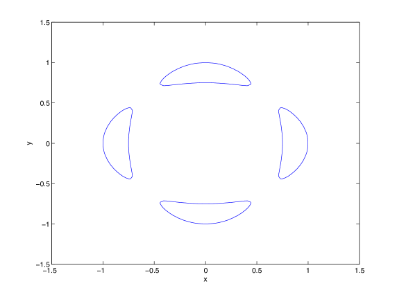
Figure 1. Real ovals of the Trott curve (5.1), an M-curve of genus 3.

Our computed matrices of $\tilde{\mathcal{A}}$ and $\tilde{\mathcal{B}}$-periods denoted by aper and bper respectively read

aper =

  -0.0000 + 0.0235i  -0.0000 + 0.0138i  -0.0000 + 0.0138i
        0 + 0.0000i   0.0000 + 0.0277i        0 + 0.0000i
  -0.0315            -0.0000 + 0.0000i   0.0250 - 0.0000i

bper =

  -0.0315 + 0.0235i  -0.0000 + 0.0138i  -0.0250 + 0.0138i
  -0.0000 + 0.0000i  -0.0250 + 0.0277i   0.0250 - 0.0000i
  -0.0000 - 0.0235i   0.0000 + 0.0138i        0 + 0.0138i.

For this the algorithm produces as expected $\mathbb{H}=0$ and $Q$ of (3.34) the identity matrix. The symplectic transformation found by the algorithm via (3.22) and (3.23) has the form

    [A,B,C,D] =

     0     1     0     0    -1     0     0     1     0     0     0     0
     1     0     0    -1     0     0     1     0     0     0     0     0
     0     0     1     0     0     0     0     0     0     0     0     1.

Since we will not actually use the matrices $A,B,C,D$ in this article, and since they follow for given periods from $\mathbb{H}$ and $Q$ via (3.22) and (3.23) we will only give them for this example. However they are needed e.g. for the study of algebro-geometric solutions to integrable equations as KP and DS as in [27].

The Klein curve given by the equation

(5.2) $$y^{7}-x(x-1)^{2}=0$$

has the maximal number of automorphisms (168) of a genus 3 curve. The computed periods read

aper =

  -0.9667 + 0.7709i   0.9667 + 0.2206i   0.9667 - 2.0073i
  -1.2054 - 0.2751i  -0.4302 + 0.8933i  -1.7419 + 1.3891i
  -0.4302 - 0.8933i   1.7419 + 1.3891i  -1.2054 + 0.2751i

bper =

  -2.7085 - 0.6182i  -0.2387 + 0.4958i   1.3969 - 1.1140i
  -2.1721 - 1.7322i   0.5365 - 0.1224i  -0.7752 - 1.6097i
   0.9667 + 0.2206i  -0.9667 + 2.0073i  -0.9667 + 0.7709i.

The algorithm finds

H =

     1     0     0
     0     1     0
     0     0     1
Q =

     1     1     1
     0     0     1
     0     1     0.

Therefore, the topological type of the curve is $(3,1,1)$, namely, the curve has genus $3$, one real oval (as can be also seen in Fig. 2) and is non-dividing.

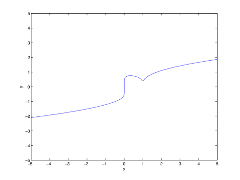
Figure 2. Real variety of the Klein curve (5.2), the curve with the maximal number of automorphisms in genus 3.

The Fermat curve

(5.3) $$y^{n}+x^{n}+1=0$$

has for $n=4$ the topological type $(3,0,1)$. This is confirmed by the algorithm. For the periods

aper =

   0.9270 + 0.0000i   0.0000 - 0.9270i   0.0000 - 0.9270i
  -0.0000 + 0.0000i   0.0000 + 0.0000i   0.0000 - 1.8541i
        0 + 0.9270i  -0.9270 + 0.0000i   0.0000 - 0.9270i

bper =

   0.9270 + 0.9270i   0.9270 - 0.9270i   0.0000 + 0.0000i
   0.0000            -0.9270 + 0.9270i   0.9270 - 0.9270i
  -0.9270 + 0.0000i   0.0000 - 0.9270i   0.0000 - 0.9270i

we find

H =

     0     1     0
     1     0     0
     0     0     0


Q =

     1     0     0
     0     0     1
     0     1     0

in accordance with the expectation. For $n=5$ the curve has genus 6. We find with

aper =

  Columns 1 through 4

  -0.1623 + 0.4995i  -0.1890 + 0.5817i  -0.1623 + 0.4995i   0.4948 + 0.3595i
  -0.3246 - 0.0000i  -0.3780 + 0.0000i  -0.3246 + 0.0000i   0.9896 - 0.0000i
  -0.4249 + 0.3087i  -0.0722 - 0.2222i   0.5252 - 0.0000i   0.6116 - 0.0000i
  -0.4249 - 0.3087i   0.1890 - 0.1373i   0.1623 + 0.4995i  -0.4948 + 0.3595i
   0.1003 - 0.3087i  -0.3058 + 0.2222i   0.3246            -0.9896 - 0.0000i
   0.5252 + 0.0000i  -0.4948 - 0.3595i   0.1623 + 0.4995i  -0.4948 + 0.3595i

  Columns 5 through 6

   0.4948 + 0.3595i   0.4249 - 0.3087i
   0.9896 - 0.0000i   0.8498 - 0.0000i
   0.1890 - 0.5817i   1.1125 + 0.8082i
   0.1890 + 0.5817i  -0.4249 - 1.3078i
   0.8006 + 0.5817i  -0.2626 - 0.8082i
   0.6116 - 0.0000i   0.1623 - 0.4995i

bper =

  Columns 1 through 4

  -0.6875 + 0.4995i  -0.8006 + 0.5817i  -0.6875 + 0.4995i  -0.1168 + 0.3595i
   0.1003 - 0.3087i   0.1168 - 0.3595i   0.1003 - 0.3087i   0.8006 + 0.5817i
  -0.6875 - 0.4995i   0.3058 - 0.2222i   0.2626 + 0.8082i   0.3058 - 0.2222i
  -0.1623 - 0.4995i   0.2336 + 0.0000i  -0.1623 + 0.4995i   0.4948 + 0.3595i
   0.4249 - 0.3087i  -0.6116 - 0.0000i   0.4249 + 0.3087i  -0.1890 - 0.5817i
  -0.1623 + 0.4995i   0.4948 - 0.3595i  -0.5252            -0.6116

  Columns 5 through 6

  -0.1168 + 0.3595i  -0.1003 - 0.3087i
   0.8006 + 0.5817i   0.6875 - 0.4995i
  -0.1168 - 0.3595i   0.2626 + 0.8082i
   0.4948 - 0.3595i   1.3751 - 0.0000i
  -0.1890 + 0.5817i  -0.5252 + 0.0000i
   0.4948 + 0.3595i  -0.1623 - 0.4995i

the matrices

H =

     1     0     0     0     0     0
     0     1     0     0     0     0
     0     0     1     0     0     0
     0     0     0     1     0     0
     0     0     0     0     1     0
     0     0     0     0     0     1


Q =

     1     0     0     0     0     0
     1     0     0     1     0     0
     0     0     0     0     1     0
     0     0     1     0     1     0
     0     1     1     0     1     0
     0     0     1     0     1     1.

This implies that there is one real oval as can be also seen in Fig. 3, and the curve is non-dividing. This corresponds to $(g,k,a)=(6,1,1)$.

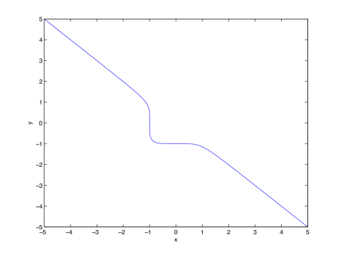
Figure 3. Real variety of the Fermat curve (5.3) for $n=5$.

For the curve

(5.4) $$y^{3}-2x^{3}y-x^{9}=0$$

of genus 3 we have

aper =

   0.4021 - 0.6964i  -0.6748 - 1.1688i   0.5985 + 1.0367i
  -0.4764 - 0.9006i   1.5026 - 0.1823i   2.0418 + 0.5711i
  -1.5598 - 0.9006i   0.3157 - 0.1823i  -0.9892 + 0.5711i

bper =

   1.1577 + 0.2041i   0.3591 - 0.9865i   0.3907 + 0.4656i
   0.5417 - 0.3128i   0.5934 + 0.3426i   1.5155 + 0.8750i
   0.6160 + 0.1086i  -0.2344 + 0.6439i  -1.1249 - 1.3406i

which leads to

H =

     1     0     0
     0     1     0
     0     0     1


Q =

     1     1     1
     0     0     1
     0     1     0.

This gives the topological type $(3,1,1)$. In particular, the number of real ovals equals one. The real variety of the curve, which has a self intersection and a cusp, can be seen in Fig. 4.

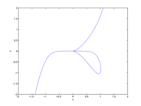
Figure 4. Real variety of the curve (5.4).

The curve

(5.5) $$-180x^{5}+396yx^{4}-307x^{3}y^{2}+107x^{2}y^{3}+273x^{3}-318x^{2}y-17xy^{4}+117xy^{2}-68x+y^{5}-12y^{3}+19y=0$$

is known (see [12]) to be a dividing curve of genus 6. In fact we get for

aper =

  Columns 1 through 4

   0.0414 + 0.0278i  -0.0345 + 0.0272i  -0.0979 + 0.0264i  -0.3041 + 0.0603i
  -0.1149 - 0.0446i   0.0000 - 0.0000i   0.0532 - 0.0226i   0.0000 - 0.0000i
   0.1149 + 0.0169i  -0.0000 + 0.0544i  -0.0532 - 0.0805i  -0.0000 + 0.1206i
   0.0000 - 0.0111i   0.0000 + 0.0183i   0.0000 - 0.0303i   0.0000 + 0.1114i
   0.0820 - 0.0278i   0.0000 + 0.0000i  -0.0527 - 0.1031i   0.0000 + 0.0000i
  -0.0820 - 0.0000i  -0.0000 - 0.0544i   0.0527 - 0.0000i  -0.0000 - 0.1206i

  Columns 5 through 6

  -0.5369 + 0.0872i  -2.8149 + 0.5433i
   0.2427 + 0.0099i   0.7641 + 0.0357i
  -0.2427 - 0.2372i  -0.7641 - 0.5381i
   0.0000 - 0.1843i   0.0000 - 1.1224i
  -0.0881 - 0.2274i  -0.1275 - 0.5024i
   0.0881 - 0.0000i   0.1275 - 0.0000i

bper =

  Columns 1 through 4

   0.0414 + 0.0278i  -0.0345 - 0.0094i  -0.0979 + 0.0264i  -0.3041 - 0.1626i
  -0.0089 - 0.1009i  -0.0666 + 0.0180i   0.1091 - 0.0733i  -0.1162 + 0.0046i
  -0.0089 - 0.0563i  -0.0666 - 0.0180i   0.1091 - 0.0507i  -0.1162 - 0.0046i
   0.0320 - 0.0000i   0.0000 - 0.0183i   0.1425 - 0.0000i   0.0000 - 0.1114i
   0.1060 + 0.0286i   0.0666 + 0.0724i   0.0559 - 0.0525i   0.1162 + 0.1252i
  -0.0580 + 0.0160i   0.0666 - 0.0363i   0.1614 + 0.0751i   0.1162 - 0.1160i

  Columns 5 through 6

  -0.5369 + 0.0872i  -2.8149 + 0.5433i
   0.3380 - 0.1055i   0.9555 - 0.2619i
   0.3380 - 0.1154i   0.9555 - 0.2976i
   0.8311 - 0.0000i   4.8657 - 0.0000i
   0.0954 - 0.1120i   0.1914 - 0.2048i
   0.2716 + 0.1021i   0.4464 + 0.1691i

the matrices

    H =

         0     1     0     0     0     0
         1     0     0     0     0     0
         0     0     0     1     0     0
         0     0     1     0     0     0
         0     0     0     0     0     0
         0     0     0     0     0     0


    Q =

         1     0     0     0     0     0
         0     1     0     0     0     0
         1     1     1     0     0     0
         0     1     0     0     1     0
         0     0     0     1     0     0
         0     0     0     0     1     1.

This means that it is a dividing curve with 3 real ovals, which is, however, not obvious from Fig. 5. The topological type is $(6,3,0)$.

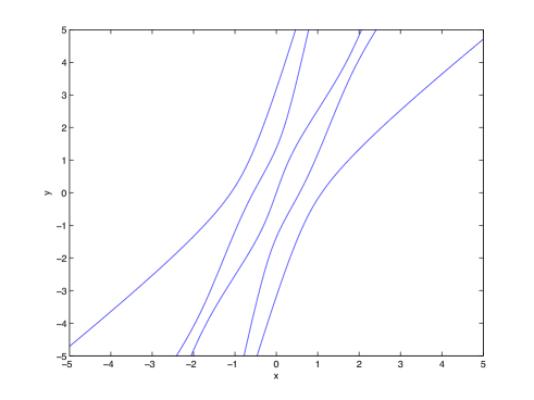
Figure 5. Real variety of the curve (5.5).

6. Outlook

The algorithm presented in this paper allows the transformation of an arbitrary canonical homology basis to a form adapted to the underlying symmetry, here the anti-holomorphic involution. This permits to find a basis satisfying relation (2.6). A similar condition can be imposed for any involution, and the algorithm presented here can be easily adapted to that case.

In general, the presence of symmetries allows to significantly simplify the Riemann matrix of a surface, but only in a homology basis adapted to the symmetries, for instance in a basis such that the $A$-cycles are invariant under symmetry operations, see [3] and [5] for the Klein curve. The latter reference uses an approach to this problem based on Comessati’s theorem [7] via two pieces of software, extcurves and CyclePainter. It will be the subject of further work to generalize the algorithm to symmetry groups beyond involutions. In a first step it would be interesting to extend the approach presented in this paper to automorphisms $\tau$ satisfying $\tau^{n}=id$ with $n>2$.

References

- [1] V. I. Arnold, The situation of ovals of real plane algebraic curves, the involutions of four-dimensional smooth manifolds, and the arithmetic of integral quadratic forms, Funkcional. Anal. i Prilozen 5, 1–9 (1971).
- [2] D. S. Arnon and S. McCallum, A polynomial time algorithm for the topological type of a real algebraic curve, Journal of Symbolic Computation, 5:213–236 (1988).
- [3] E. Belokolos, A. Bobenko, V. Enolskii, A. Its, V. Matveev, Algebro-geometric approach to nonlinear integrable equations, Springer Series in nonlinear dynamics (1994).
- [4] A.I. Bobenko, C. Klein, (ed.), Computational Approach to Riemann Surfaces, Lect. Notes Math. 2013 (2011).
- [5] H. W. Braden, T.P. Northover, Klein’s Curve, J. Phys. A 43, 434009 (2010).
- [6] H. Braden, V. Enolskii, T. Northover, Maple packages extcurves and CyclePainter, available at gitorious.org.
- [7] A. Comessati, Sulla connessione delle superficie algebriche reali, Annali di Mat. (3) 23, 215–283 (1915).
- [8] M. Coste, M.-F. Roy, Thom’s lemma, the coding of real algebraic numbers and the computation of the topology of semi-algebraic sets, Journal of Symbolic Computation, 5:121–129 (1988).
- [9] B. Deconinck, M. van Hoeij, Computing Riemann matrices of algebraic curves, Physica D, 28, 152–153 (2001).
- [10] B. Deconinck, M. Heil, A. Bobenko, M. van Hoeij, M. Schmies, Computing Riemann Theta Functions, Mathematics of Computation 73, 1417 (2004).
- [11] B. Deconinck, M. Patterson, Computing with plane algebraic curves and Riemann surfaces: the algorithms of the Maple package “algcurves”, in A.I. Bobenko, C. Klein, (ed.), Computational Approach to Riemann Surfaces, Lect. Notes Math. 2013 (2011).
- [12] B.A. Dubrovin, Matrix finite-zone operators, Revs. Sci. Tech. 23, 20–50 (1983).
- [13] B. Dubrovin, S. Natanzon, Real theta-function solutions of the Kadomtsev-Petviashvili equation, Math. USSR Ivestiya, 32:2, 269–288 (1989).
- [14] H. Feng, Decomposition and Computation of the Topology of Plane Real Algebraic Curves, Ph.D. thesis, The Royal Institute of Technology, Stockholm (1992).
- [15] J. Frauendiener, C. Klein, Hyperelliptic theta functions and spectral methods, J. Comp. Appl. Math. (2004).
- [16] J. Frauendiener, C. Klein, Hyperelliptic theta functions and spectral methods: KdV and KP solutions, Lett. Math. Phys., Vol. 76, 249–267 (2006).
- [17] J. Frauendiener, C. Klein, Algebraic curves and Riemann surfaces in Matlab, in A. Bobenko and C. Klein (ed.), Riemann Surfaces–Computational Approaches, Lecture Notes in Mathematics Vol. 2013 (Springer) (2011).
- [18] A. Gabard, Sur la topologie et la g om trie des courbes alg briques r elles, Ph.D. Thesis (2004).
- [19] L. Gonzalez-Vega, I. Necula, Efficient topology determination of implicitly defined algebraic plane curves, Computer Aided Geometric Design, 19:719–743 (2002).
- [20] D.A. Gudkov, Complete topological classification of the disposition of ovals of a sixth order curve in the projective plane, Gor’kov. Gos. Univ. Ucen. Zap. Vyp., 87:118–153 (1969).
- [21] A. Harnack, Ueber die Vieltheiligkeit der ebenen algebraischen Curven, Math. Ann., 10, 189–199 (1876).
- [22] J. Hafner and K. McCurley, Asymptotically fast triangularization of matrices over rings, SIAM J. Comput. 20, 1068-1083 (1991).
- [23] D. Hilbert, ber die reellen Z ge algebraischen Kurven, Math. Ann., 38, 115–138 (1891).
- [24] D. Hilbert, Mathematische Probleme, Arch. Math. Phys., 1:43–63, (German) (1901).
- [25] H. Hong, An efficient method for analyzing the topology of plane real algebraic curves, Mathematics and Computers in Simulation, 42:571–582 (1996).
- [26] C. Kalla, New degeneration of Fay’s identity and its application to integrable systems, preprint arXiv:1104.2568v1 (2011).
- [27] C. Kalla, C. Klein, On the numerical evaluation of algebro-geometric solutions to integrable equations, Nonlinearity 25 569-596 (2012).
- [28] F. Klein, On Riemann’s theory of algebraic functions and their integrals, Dover (1963).
- [29] S. Lang, Algebra, Revised Third Edition, Springer-Verlag, New York (2002).
- [30] T. Malanyuk, Finite-gap solutions of the Davey-Stewartson equations, J. Nonlinear Sci, 4, No. 1, 1–21 (1994).
- [31] I. Petrovsky, On the topology of real plane algebraic curves, Ann. Math., 39, No. 1, 187–209 (1938).
- [32] K. Rohn, Die Maximalzahl und Anordnung der Ovale bei der ebenen Kurve 6. Ordnung und bei der Fläche 4. Ordnung, Math. Ann., 73, 177-229 (1913).
- [33] T. Sakkalis, The topological configuration of a real algebraic curve, Bulletin of the Australian Mathematical Society, 43:37–50 (1991).
- [34] R. Seidel, N. Wolpert, On the exact computation of the topology of real algebraic curves, In Proc 21st ACM Symposium on Computational Geometry, p 107–115 (2005).
- [35] M. Seppäłä and R. Silhol, Moduli Spaces for Real Algebraic Curves and Real Abelian Varieties, Math. Z. 201, 151-165 (1989).
- [36] C.L. Tretkoff, M.D. Tretkoff, Combinatorial group theory, Riemann surfaces and differential equations, Contemporary Mathematics, 33, 467–517 (1984).
- [37] M. Trott, Applying Groebner Basis to Three Problems in Geometry, Mathematica in Education and Research 6 (1): 15–28 (1997).
- [38] V. Vinnikov, Self-adjoint determinantal representations of real plane curves, Math. Ann. 296, 453–479 (1993).
- [39] O. Ya. Viro, Gluing of plane real algebraic curves and constructions of curves of degrees 6 and 7, Topology (Leningrad, 1982), Lecture Notes in Math., vol. 1060, Springer, Berlin, pp. 187–200 (1984).