A New Triangular Spectral Element Method I: Implementation and Analysis on a Triangle

Abstract.

This paper serves as our first effort to develop a new triangular spectral element method (TSEM) on unstructured meshes, using the rectangle-triangle mapping proposed in the conference note [24]. Here, we provide some new insights into the originality and distinctive features of the mapping, and show that this transform only induces a logarithmic singularity, which allows us to devise a fast, stable and accurate numerical algorithm for its removal. Consequently, any triangular element can be treated as efficiently as a quadrilateral element, which affords a great flexibility in handling complex computational domains. Benefited from the fact that the image of the mapping includes the polynomial space as a subset, we are able to obtain optimal $L^{2}$- and $H^{1}$-estimates of approximation by the proposed basis functions on triangle. The implementation details and some numerical examples are provided to validate the efficiency and accuracy of the proposed method. All these will pave the way for developing an unstructured TSEM based on, e.g., the hybridizable discontinuous Galerkin formulation.

1. Introduction

The spectral element method (SEM), originated from Patera [28], integrates the unparalleled accuracy of spectral methods with the geometric flexibility of finite elements, and also enjoys a high-level parallel computer architecture. Nowadays, it has become a pervasive numerical technique for simulating challenging problems in complex domains [9, 3]. While the classical SEM on quadrilateral/hexahedral elements (QSEM) exhibits the advantages of using tensorial basis functions and naturally diagonal mass matrices, the need for high-order methods on unstructured meshes with robust adaptivity spawns the development of triangular/tetrahedral spectral elements. In general, research efforts along this line fall into three trends: (i) nodal TSEM based on high-order polynomial interpolation on special interpolation points [5, 17, 33]; (ii) modal TSEM based on the Koornwinder-Dubiner polynomials [21, 10, 19]; and (iii) approximation by non-polynomial functions [31, 23, 4].

The question of how to construct “good” interpolation points for stable high-order polynomial interpolation on the triangle is still quite subtle and somehow open. The strict analogy of the Gauss-Lobatto integration rule on quadrilaterals/hexahedra does not exist on triangles [16], though a “relaxed” rule can be constructed in the sense of [37]. We refer to [27] for an up-to-date review and a very dedicated comparative study of various criteria for constructing workable interpolation points on the triangle. In general, such points have low degree of precision (i.e., exactness for integration of polynomials), and this motivates [26] the use of a different set of points for integration, which are mapped from the Gauss points on the reference square via the Duffy’s transform [11]. The development of TSEM using Koornwinder-Dubiner polynomials as modal basis functions, generated by the rectangle-triangle mapping (i.e., the Duffy’s transform), can be best attested to by the monograph [19] and spectral-element package NekTar (http://www.nektar.info/). The analysis of this approach can be found in e.g., [14, 29, 22, 6]. However, the main drawbacks of this approach lie in that the interpolation points are unfavorably clustered near one vertex of the triangle, and there is no corresponding nodal basis, making it complicate to implement. To overcome the second difficulty, a full tensorial rational approximation on triangles was proposed in [31] for elliptic problems, and extended to the Navier-Stokes problem in [4]. This approach still builds on the collapsed Duffy’s transform with clustered grids.

It is important to point out that the Duffy’s transform not only leads to undesirable distributions of interpolation/quadrature points, but also requires modifying the tensorial polynomial basis to meet the underlying consistency conditions (analogous to “pole conditions” in polar/spherical coordinates) induced by the singularity of the transform. Our mind-set is therefore driven by searching for a method based on a different rectangle-triangle mapping that can lead to favorable distributions of interpolation/quadrature points on the triangle without loss of accuracy and efficiency of implementation. With this in mind, we introduced in the conference note [24] a new mapping that pulls one side (at the middle point) of the triangle to two sides of the rectangle (cf. Figure 1.1 (a)), and results in much more desirable distributions of the mapped LGL points (cf. Figure 1.1 (c) vs. (d)). Moreover, this mapping is one-to-one.

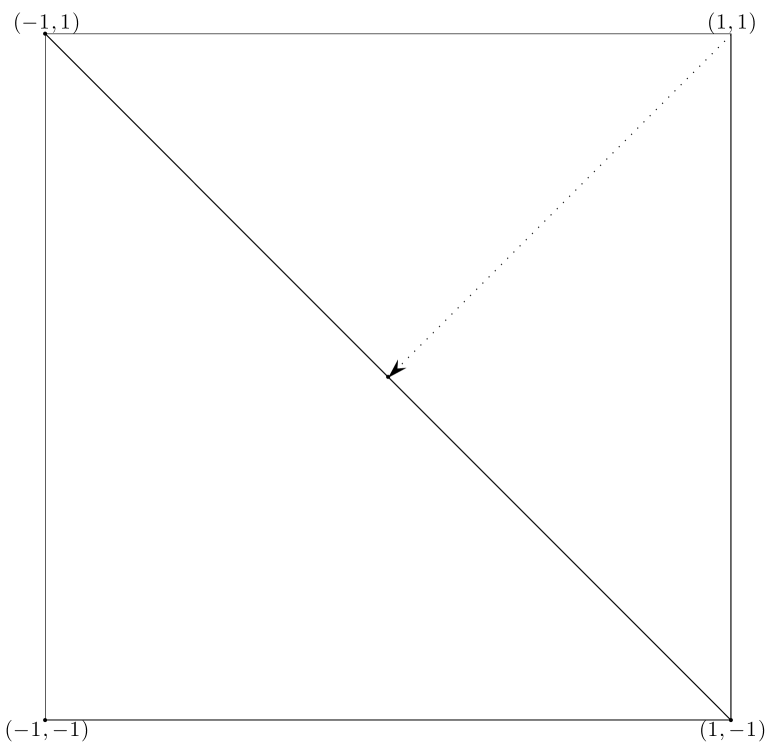
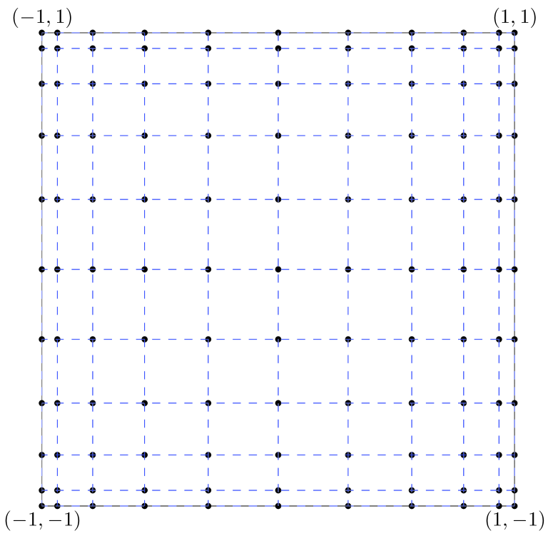
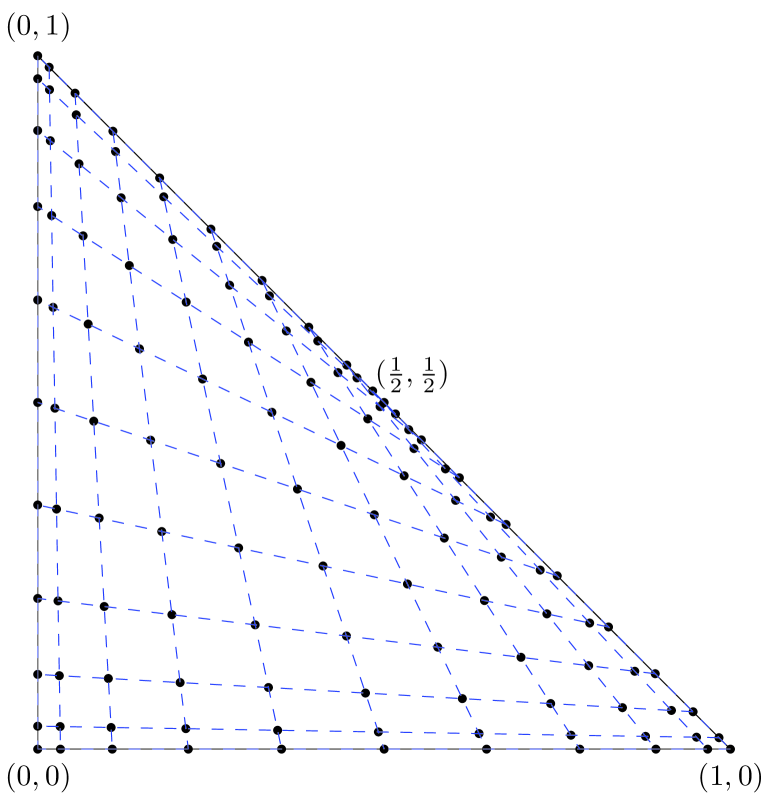
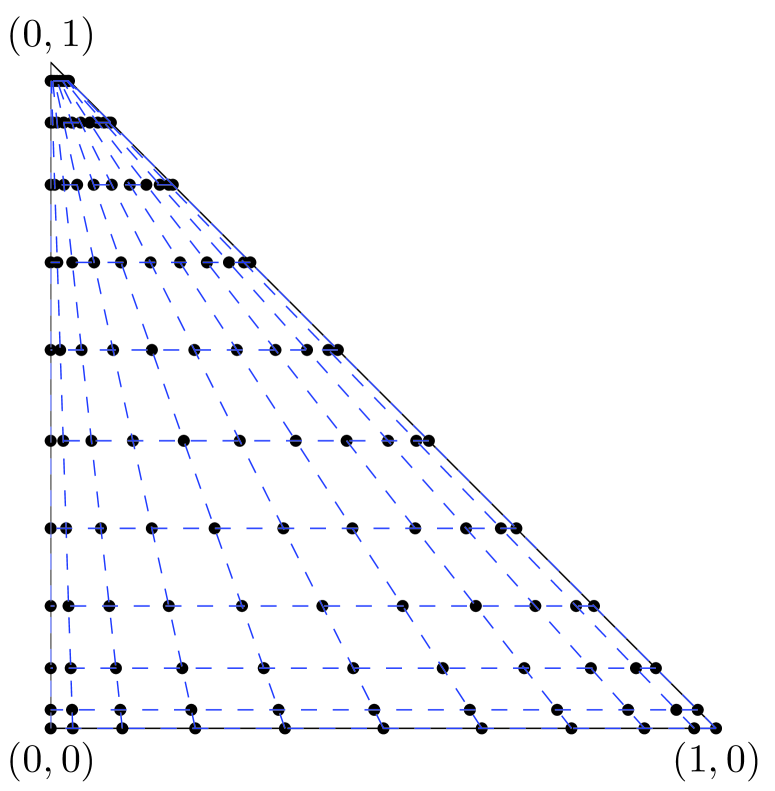
Figure 1.1. (a). ${\bigtriangleup}\leftrightarrow{\Box}$ mapping; (b). tensorial Legendre-Gauss-Lobatto (LGL) points on ${\Box}$; (c). mapped LGL grids on ${\bigtriangleup}$; (d). mapped LGL grids on ${\bigtriangleup}$ using the Duffy’s transform.

The purposes of this paper are threefold: (i) have some new insights into this mapping; (ii) demonstrate that the singularity of the mapping is of logarithmic type, which can be fully removed; and (iii) derive optimal error estimates for approximation by the associated basis functions. This work will pave the way for developing a new TSEM on unstructured meshes, which will be explored in the second part. It also brings about an important viewpoint that any triangular element can be mapped to the reference square via a composite of the rectangle-triangle mapping and an affine mapping, and with the successful removal of the singularity, the triangular element can be treated as efficiently as a quadrilateral element. One implication is that this allows a mixture of triangular and quadrilateral elements, so one can handle more complex domains with more regular computational meshes, e.g., by tiling the triangular elements along the boundary of the domain. More importantly, for general unstructured triangular meshes, we can formulate the underlying variational problems using the recently enhanced hybridizable discontinuous Galerkin methods [8, 20, 25]. We expect that the QSEM will enjoy a minimal communication between elements, and a minimum number of globally coupled degree of freedoms, and allow for implementing a large degree of nonconformity across elements (e.g., the hanging nodes and mortaring techniques). We leave this development to the second part after this work.

The rest of this paper is organized as follows. In Section 2, we present some new insights of the rectangle-triangle mapping. In Section 3, we introduce the basis functions and the efficient algorithm for computing the stiffness and mass matrices with an emphasis on how to remove the singularity of the rectangle-triangle transform. We derive some optimal approximation results in Section 4, followed by numerical results on a triangle in Section 5.

2. The rectangle-triangle mapping

We collect in this section some properties of the rectangle-triangle mapping introduced in [24], and provide some insightful perspectives on this transform.

2.1. The rectangle-triangle mapping

Throughout the paper, we denote by

$${\bigtriangleup}:=\big{\{}(x,y):\,0<x,y,x+y<1\big{\}},\quad{\Box}:=\big{\{}(\xi,\eta):\,-1<\xi,\eta<1\big{\}},$$

the reference triangle and the reference square, respectively. The rectangle-triangle transform (cf. [24]) $T:{\Box}\to{\bigtriangleup},$ takes the form

$$x=\frac{1}{8}(1+\xi)(3-\eta),\quad y=\frac{1}{8}(3-\xi)(1+\eta),\quad\forall\;(\xi,\eta)\in{{\Box}},$$ (2.1)

with the inversion $T^{-1}:{\bigtriangleup}\to{\Box}:$

$$\begin{cases}\xi=1+(x-y)-\sqrt{(x-y)^{2}+4(1-x-y)},\\[3.99994pt] \eta=1-(x-y)-\sqrt{(x-y)^{2}+4(1-x-y)},\end{cases}$$ (2.2)

for any $(x,y)\in{{\bigtriangleup}}.$ It maps the vertices $(-1,-1),(1,-1)$ and $(-1,1)$ of the square ${\Box}$ to the vertices $(0,0),\,(1,0)$ and $(0,1)$ of the triangle ${\bigtriangleup}$, respectively, while the middle point $(1/2,1/2)$ of the hypotenuse is the image of the vertex $(1,1)$ of ${\Box}$. In other words, this mapping deforms two edges ($\xi=1$ and $\eta=1$) of ${\Box}$ into the hypotenuse of ${\bigtriangleup}$, see Figure 1.1 for illustration.

Under this mapping, we have

$$\frac{\partial x}{\partial\xi}=\frac{3-\eta}{8},\quad\frac{\partial x}{\partial\eta}=-\frac{1+\xi}{8},\quad\frac{\partial y}{\partial\xi}=-\frac{1+\eta}{8},\quad\frac{\partial y}{\partial\eta}=\frac{3-\xi}{8},$$ (2.3)

and the Jacobian is given by

$$J=\det\left(\frac{\partial(x,y)}{\partial(\xi,\eta)}\right)=\frac{2-\xi-\eta}{16}=\frac{\sqrt{(x-y)^{2}+4(1-x-y)}}{8}:=\frac{\chi}{8}.$$ (2.4)

For convenience of presentation, we use the handy notation:

$$\widetilde{\nabla}=(\partial_{\xi},\partial_{\eta}),\quad\widetilde{\nabla}^{\bot}=(-\partial_{\eta},\partial_{\xi}),\quad\widetilde{\nabla}^{\intercal}=(1-\xi)\partial_{\xi}-(1-\eta)\partial_{\eta},$$ (2.5)

where we put “ $\widetilde{~{}}$ ” to distinguish them from the differential operators in $(x,y).$ Given $u(x,y)$ on ${\bigtriangleup},$ we define the transformed function: $\tilde{u}(\xi,\eta)=(u\circ T)(\xi,\eta)=u(x,y),$ and likewise for $\tilde{v},$ etc.. Then we have

$$({u},{v})_{{\bigtriangleup}}=\int\int_{\bigtriangleup}u(x,y)v(x,y)\mathrm{d}x\mathrm{d}y=\int\int_{\Box}\tilde{u}(\xi,\eta)\tilde{v}(\xi,\eta)J\,\mathrm{d}\xi\mathrm{d}\eta.$$ (2.6)

Moreover, one verifies that

$$\nabla u=\left(\partial_{x}u,\partial_{y}u\right)=\chi^{-1}\big{(}2(\widetilde{\nabla}\cdot\tilde{u})+(\widetilde{\nabla}^{\intercal}\tilde{u}),\,2(\widetilde{\nabla}\cdot\tilde{u})-(\widetilde{\nabla}^{\intercal}\tilde{u})\big{)},$$ (2.7)

and

$$\begin{split}\left(\nabla u,\nabla v\right)_{{\bigtriangleup}}&=\int\int_{\Box}\big{(}\widetilde{\nabla}\cdot\tilde{u}\big{)}\big{(}\widetilde{\nabla}\cdot\tilde{v}\big{)}\chi^{-1}\mathrm{d}\xi\mathrm{d}\eta+\frac{1}{4}\int\int_{\Box}\big{(}{\widetilde{\nabla}}^{\intercal}\tilde{u}\big{)}\big{(}\widetilde{\nabla}^{\intercal}\tilde{v}\big{)}\chi^{-1}\mathrm{d}\xi\mathrm{d}\eta.\end{split}$$ (2.8)

We observe from (2.7)-(2.8) that if $\nabla u$ is continuous at the middle point $\left({1}/{2},{1}/{2}\right)$ of the hypotenuse of ${\bigtriangleup}$, there automatically holds (note: $({\widetilde{\nabla}}^{\intercal}\tilde{u})|_{(1,1)}=0$):

$$\big{(}\widetilde{\nabla}\cdot\tilde{u}\big{)}|_{(1,1)}=\left.\left(\frac{\partial\tilde{u}}{\partial\xi}+\frac{\partial\tilde{u}}{\partial\eta}\right)\right|_{(1,1)}=0,$$ (2.9)

which is referred to as the consistency condition, and can be viewed as an analogy of the pole condition in the polar/spherical coordinates. In general, we have to build the condition (2.9) in the approximation space so as to obtain high-order accuracy, which therefore results in the reduction of dimension and modification of the usual basis functions (cf. [24]).

One important goal of this paper is to demonstrate that this singularity can be removed, thanks to the observation:

$$\int\int_{{\Box}}\frac{1}{2-\xi-\eta}\,\mathrm{d}\xi\mathrm{d}\eta=4\ln 2,$$ (2.10)

which implies that for any $f\in C(\overline{\Box}),$

$$\Big{|}\int\int_{{\Box}}\frac{f(\xi,\eta)}{2-\xi-\eta}\,\mathrm{d}\xi\mathrm{d}\eta\Big{|}\leq 4M\ln 2,$$ (2.11)

where $M=\max_{\overline{\Box}}|f(\xi,\eta)|.$ In particular, the coordinate singularity can be eliminated, if $f$ is a polynomial on ${\Box}$ (see Subsection 3.2).

Now, we present other important features of this mapping. Hereafter, let $I=(-1,1),$ and for any integer $N\geq 1,$ let ${P}_{N}(I)$ be the set of all algebraic polynomials of degree at most $N$. Denote by

$${\mathcal{P}}_{N}({\bigtriangleup}):={\rm span}\big{\{}x^{i}y^{j}:0\leq i+j\leq N\big{\}},\quad{\mathcal{Q}}_{N}({\Box}):=(P_{N}(I))^{2}.$$ (2.12)

The following property shows the correspondence between two polynomial spaces.

Proposition 2.1.

We have

• ${\mathcal{P}}_{N}({\bigtriangleup})\circ T\subset{\mathcal{Q}}_{N}({\Box}).$

• ${\mathcal{Q}}_{N}({\Box})=\big{(}{\mathcal{P}}_{N}({\bigtriangleup})\circ T\big{)}\oplus\chi\big{(}{\mathcal{P}}_{N-1}({\bigtriangleup})\circ T\big{)}.$

Here, $T$ is the rectangle-triangle transform defined by (2.1), and $\chi=(2-\xi-\eta)/2.$

Proof.

We find from (2.1) that for $0\leq i+j\leq N,$

$$x^{i}y^{j}=\Big{(}\frac{1+\xi}{2}\Big{)}^{i}\Big{(}\frac{3-\eta}{4}\Big{)}^{i}\Big{(}\frac{3-\xi}{4}\Big{)}^{j}\Big{(}\frac{1+\eta}{2}\Big{)}^{j}\in{\mathcal{Q}}_{N}({\Box}).$$

This leads to the inclusion in (i).

We see that for $0\leq i+j\leq N-1,$

$$x^{i}y^{j}\chi=\Big{(}\frac{1+\xi}{2}\Big{)}^{i}\Big{(}\frac{3-\eta}{4}\Big{)}^{i}\Big{(}\frac{3-\xi}{4}\Big{)}^{j}\Big{(}\frac{1+\eta}{2}\Big{)}^{j}\frac{2-\xi-\eta}{2}\in{\mathcal{Q}}_{N}({\Box}),$$

which implies $\chi\big{(}{\mathcal{P}}_{N-1}({\bigtriangleup})\circ T\big{)}\subset{\mathcal{Q}}_{N}({\Box}).$

It remains to prove ${\mathcal{Q}}_{N}({\Box})\subset\big{(}{\mathcal{P}}_{N}({\bigtriangleup})\circ T\big{)}\oplus\chi\big{(}{\mathcal{P}}_{N-1}({\bigtriangleup})\circ T\big{)},$ which we will show by induction. Firstly, by (2.2), it is true for $\xi,\eta,$ so is $\xi\eta,$ since $\xi\eta=5-4x-4y-2\chi.$ Now, assume that it holds for $\xi^{i}\eta^{j}$ with $0\leq i,j\leq N-1$. Then, for $0\leq i,j\leq N$, we find that $\xi^{N}\eta^{j}=\xi(\xi^{N-1}\eta^{j})$, $\xi^{i}\eta^{N}=\eta(\xi^{i}\eta^{N-1})$, and $\xi^{N}\eta^{N}=(\xi\eta)(\xi^{N-1}\eta^{N-1})$ are all of the form $(a+bx+cy+d\chi)(p(x,y)+q(x,y)\chi)$, where $a,b,c,d$ are constants, $p\in\mathcal{P}_{N-1}({\bigtriangleup})$ and $q\in\mathcal{P}_{N-2}({\bigtriangleup})$. It is apparent that

$$(a+bx+cy+d\chi)(p+q\chi)=(a+bx+cy)p+dp\chi+(a+bx+cy)q\chi+dq\chi^{2}$$

$$\quad\overset{(\ref{best_map_inv})}{=}(a+bx+cy)p+d\big{(}(x-y)^{2}+4(1-x-y)\big{)}q+\big{(}dp+(a+bx+cy)q\big{)}\chi.$$

Since $(a+bx+cy)p,d\chi^{2}q\in\mathcal{P}_{N}({\bigtriangleup})$ and $dp,(a+bx+cy)q\in\mathcal{P}_{N-1}({\bigtriangleup})$, we have

$$\xi^{N}\eta^{j},\xi^{i}\eta^{N},\xi^{N}\eta^{N}\in\big{(}{\mathcal{P}}_{N}({\bigtriangleup})\circ T\big{)}\oplus\chi\big{(}{\mathcal{P}}_{N-1}({\bigtriangleup})\circ T\big{)},$$

for all $0\leq i,j\leq N$. This completes the induction.  

In what follows, let $\omega>0$ be a generic weight function on $\Omega={\bigtriangleup}$ or ${\Box}.$ The weighted Sobolev space $H^{r}_{\omega}(\Omega)$ with $r\geq 0$ is defined as in Adams [1], and its norm and semi-norm are denoted by $\|\cdot\|_{r,\omega,\Omega}$ and $|\cdot|_{r,\omega,\Omega},$ respectively. In particular, if $r=0,$ we denote the inner product and norm of $L^{2}_{\omega}(\Omega)$ by $(\cdot,\cdot)_{\omega,\Omega}$ and $\|\cdot\|_{\omega,\Omega},$ respectively. Moreover, if $\omega\equiv 1,$ we drop it from the notation.

Proposition 2.2.

For any $u\in H^{1}({\bigtriangleup}),$ we have

$$\frac{\sqrt{3}}{2}\big{\|}\widetilde{\nabla}\cdot\tilde{u}\big{\|}_{\chi^{-1},{\Box}}+\frac{\sqrt{2}}{4}\big{\|}\widetilde{\nabla}^{\bot}\cdot\tilde{u}\big{\|}_{\chi,{\Box}}\leq\big{\|}\nabla u\big{\|}_{{\bigtriangleup}}\leq\frac{\sqrt{5}}{2}\big{\|}\widetilde{\nabla}\cdot\tilde{u}\big{\|}_{\chi^{-1},{\Box}}+\frac{1}{2}\big{\|}\widetilde{\nabla}^{\bot}\cdot\tilde{u}\big{\|}_{\chi,{\Box}},$$ (2.13)

where $\chi=(2-\xi-\eta)/2,$ $\tilde{u}=u\circ T$ and the differential operators are defined in (2.5).

Proof.

By (2.8), we have

$$\big{\|}\nabla u\big{\|}_{{\bigtriangleup}}^{2}=\big{\|}\widetilde{\nabla}\cdot\tilde{u}\big{\|}^{2}_{\chi^{-1},{\Box}}+\frac{1}{4}\big{\|}\widetilde{\nabla}^{\intercal}\tilde{u}\big{\|}^{2}_{\chi^{-1},{\Box}}.$$

Then using the identity:

$$\widetilde{\nabla}^{\intercal}\tilde{u}=(1-\xi)\partial_{\xi}\tilde{u}-(1-\eta)\partial_{\eta}\tilde{u}=\frac{1}{2}\big{(}2\chi(\widetilde{\nabla}^{\bot}\cdot\tilde{u})-(\xi-\eta)(\widetilde{\nabla}\cdot\tilde{u})\big{)},$$

we obtain

$$\big{\|}\nabla u\big{\|}_{{\bigtriangleup}}^{2}=\big{\|}\widetilde{\nabla}\cdot\tilde{u}\big{\|}^{2}_{\chi^{-1},{\Box}}+\frac{1}{16}\big{\|}2\chi(\widetilde{\nabla}^{\bot}\cdot\tilde{u})-(\xi-\eta)(\widetilde{\nabla}\cdot\tilde{u})\big{\|}^{2}_{\chi^{-1},{\Box}}.$$ (2.14)

As $|\xi-\eta|\leq 2,$ we get

$$\big{\|}2\chi(\widetilde{\nabla}^{\bot}\cdot\tilde{u})-(\xi-\eta)(\widetilde{\nabla}\cdot\tilde{u})\big{\|}^{2}_{\chi^{-1},{\Box}}\leq 4\big{\|}\widetilde{\nabla}^{\bot}\cdot\tilde{u}\big{\|}_{\chi,{\Box}}^{2}+4\big{\|}\widetilde{\nabla}\cdot\tilde{u}\big{\|}_{\chi^{-1},{\Box}}^{2}.$$

Thus, the upper bound of (2.13) is a consequence of (2.14).

It is clear that

$$-4(\xi-\eta)\chi(\widetilde{\nabla}^{\bot}\cdot\tilde{u})(\widetilde{\nabla}\cdot\tilde{u})\geq-\big{(}2{\chi^{2}}|\widetilde{\nabla}^{\bot}\cdot\tilde{u}|^{2}+{2(\xi-\eta)^{2}}|\widetilde{\nabla}\cdot\tilde{u}|^{2}\big{)}.$$

Thus,

$$\big{(}2\chi(\widetilde{\nabla}^{\bot}\cdot\tilde{u})-(\xi-\eta)(\widetilde{\nabla}\cdot\tilde{u})\big{)}^{2} \geq 2{\chi^{2}}|\widetilde{\nabla}^{\bot}\cdot\tilde{u}|^{2}-(\xi-\eta)^{2}|\widetilde{\nabla}\cdot\tilde{u}|^{2}$$

$$\geq 2{\chi^{2}}|\widetilde{\nabla}^{\bot}\cdot\tilde{u}|^{2}-4|\widetilde{\nabla}\cdot\tilde{u}|^{2},$$

which implies

$$\big{\|}2\chi(\widetilde{\nabla}^{\bot}\cdot\tilde{u})-(\xi-\eta)(\widetilde{\nabla}\cdot\tilde{u})\big{\|}^{2}_{\chi^{-1},{\Box}}\geq 2\big{\|}\widetilde{\nabla}^{\bot}\cdot\tilde{u}\big{\|}_{\chi,{\Box}}^{2}-4\big{\|}\widetilde{\nabla}\cdot\tilde{u}\big{\|}_{\chi^{-1},{\Box}}^{2}.$$

Therefore, the lower bound of (2.13) follows from (2.14).  

Remark 2.1.

We find from Proposition 2.2 that under the rectangle-triangle mapping (2.1), the space $H^{1}({\bigtriangleup})$ is mapped to the weighted space on ${\Box}$:

$$\widetilde{H}^{1}_{\chi}({\Box}):=\big{\{}\tilde{u}\in L^{2}_{\chi}\!\left({\Box}\right):\widetilde{\nabla}\cdot{\tilde{u}}\in L^{2}_{\chi}\!\left({\Box}\right),\widetilde{\nabla}^{\bot}\cdot{\tilde{u}}\in L^{2}_{\chi^{-1}}\!\left({\Box}\right)\big{\}},$$ (2.15)

and vice verse.  

2.2. Some new perspectives and a comparison study

Next, we have some insights of the rectangle-triangle mapping and compare it with the Duffy’s transform [11].

Firstly, the transform (2.1) is a special case of the general mapping $T_{\theta}:{\Box}\mapsto{\bigtriangleup}:$

$$(x,y)=\left(\frac{1+\xi}{2}\frac{2-(1-\theta)(1+\eta)}{2},\frac{1+\eta}{2}\frac{2-\theta(1+\xi)}{2}\right),\quad\forall(\xi,\eta)\in{{\Box}},$$ (2.16)

with $\theta=1/2.$ We see that this mapping pulls the hypotenuse of ${\bigtriangleup}$ into two edges of ${\bigtriangleup}$ at the point $(\theta,1-\theta).$ The limiting case with $\theta=0$ reduces to the Duffy’s transform: $T_{D}:{\Box}\mapsto{\bigtriangleup}:$

$$x=\frac{1}{4}(1+\xi)(1-\eta),\quad y=\frac{1}{2}(1+\eta),\quad\forall\,(\xi,\eta)\in{\Box},$$ (2.17)

with the inverse transform: $T_{D}^{-1}:{\bigtriangleup}\mapsto{\Box}:$

$$\xi=\frac{2x}{1-y}-1,\quad\eta=2y-1,\quad\forall\,(x,y)\in{\bigtriangleup}.$$

It collapses one edge, $\eta=1$, of ${\Box}$ into the vertex $(0,1)$ of ${\bigtriangleup}.$ As the singular vertex corresponds to one edge, the Duffy’s transform is not a one-to-one mapping, as opposite to (2.1). This results in a large portion of mapped LGL points clustered near the singular vertex of ${\bigtriangleup}$ (see Figure 1.1 (d)). The Jacobian of (2.17)-(2.2) is $J=(1-\eta)/8,$ and we have

$$\nabla u=\Big{(}\frac{4}{1-\eta}\partial_{\xi}\tilde{u},\frac{2(1+\xi)}{1-\eta}\partial_{\xi}\tilde{u}+2\partial_{\eta}\tilde{u}\Big{)}.$$ (2.18)

Different from (2.9), the corresponding consistency condition of the Duffy’s transform becomes $\partial_{\xi}\tilde{u}(\xi,1)=0.$ In a distinct contrast with (2.10), the integral

$$\int\int_{{\Box}}\frac{1}{1-\eta}\,\mathrm{d}\xi\mathrm{d}\eta=\infty.$$ (2.19)

Consequently, the consistency condition has to be built in the approximation space, and much care has to taken to deal with this singularity for Duffy’s transform-based methods in terms of implementation and analysis.

Secondly, the nature of the point singularity of (2.1) is reminiscent to that of the Gordon-Hall mapping [13], which maps the reference square to the unit disc via

$$x=\frac{\xi}{\sqrt{2}}\sqrt{2-\eta^{2}},\quad y=\frac{\eta}{\sqrt{2}}\sqrt{2-\xi^{2}},\quad\forall\,(\xi,\eta)\in{\Box},$$

and whose Jacobian is $(2-\xi^{2}-\eta^{2})/\sqrt{(2-\xi^{2})(2-\eta^{2})}.$ It is clear that this transform induces singularity at four vertices of the reference square (cf. Figure 2.1). It is worthwhile to point out that the collocation scheme on the unit disc using this mapping was discussed in [15], and this mapping technique was further examined in [2].

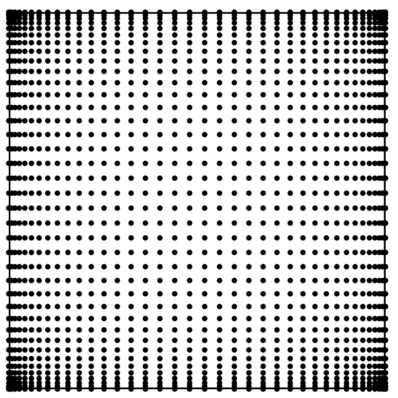
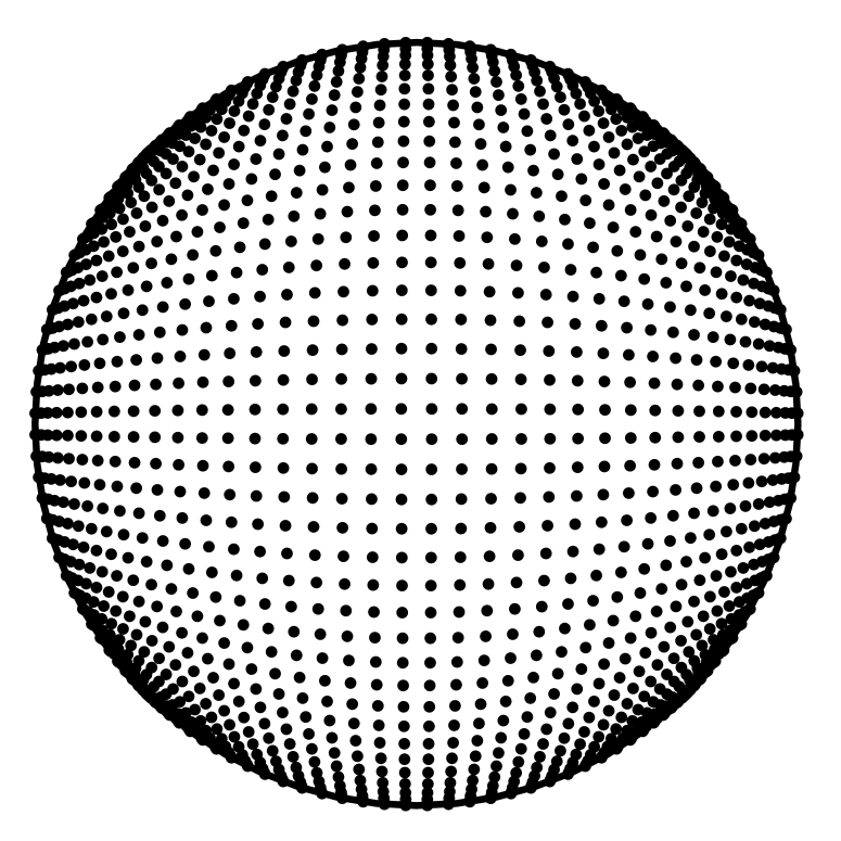
Figure 2.1. Left: tensorial Legendre-Gauss-Lobatto points on the square. Right: the corresponding mapped LGL points on the unit disc.

In addition, we find that the rectangle-triangle transform (2.1) can be derived from the symmetric mapping on ${\Box}:$

$$\hat{x}={\xi}+{\eta},\quad\hat{y}={\xi}{\eta},\quad\forall\,(\xi,\eta)\in{\Box}.$$ (2.20)

It transforms any symmetric polynomial in $(\xi,\eta)$ to a polynomial in $(\hat{x},\hat{y}),$ so it is referred to as a symmetric mapping [34]. One verifies that the image of this mapping is the curvilinear triangle (see Figure 2.2 (b)):

$${\Omega}=\big{\{}(\hat{x},\hat{y}):1-\hat{x}+\hat{y},\,1+\hat{x}+\hat{y},\,\hat{x}^{2}-4\hat{y}>0\big{\}}.$$

As the symmetric mapping (2.20), denoted by $\widehat{T}:{\Box}\mapsto\Omega,$ can not distinguish the images of $(\xi,\eta)$ and $(\eta,\xi),$ it is not one-to-one. To amend this, one may restrict the domain of $\widehat{T}$ to the upper triangle, denoted by ${\bigtriangleup}_{\rm up},$ in ${\Box}$ (see Figure 2.2 (a)), and interestingly, the square of maximum area contained in this subdomain is one-to-one mapped to the triangle of maximum area included in the curvilinear triangle $\Omega$, that is,

$$\widehat{T}:\widehat{\Box}:=(-1,0)\times(0,1)\;\longmapsto\;\;\widehat{\bigtriangleup}:=\big{\{}(\hat{x},\hat{y}):|\hat{x}|<1+\hat{y}<1\big{\}},$$ (2.21)

is a bijective mapping (see the shaded parts in Figure 2.2 (a)-(b)). For clarity of presentation, we denote the coordinate of any point in $\widehat{\Box}$ by $(\hat{\xi},\hat{\eta}).$ It is clear that the reference square ${\Box}$ and $\widehat{\Box}$ are connected by the affine mapping: $F_{1}:{\Box}\mapsto\widehat{\Box},$ of the form (see the shaded parts of Figure 2.2 (a), (c)):

$$\hat{\xi}=\frac{\xi-1}{2},\quad\hat{\eta}=\frac{1-\eta}{2},\quad\forall(\xi,\eta)\in{\Box},$$ (2.22)

and the affine mapping: $F_{2}:\widehat{\bigtriangleup}\mapsto{\bigtriangleup},$ takes the form (see the shaded parts of Figure 2.2 (b), (d)):

$$x=\frac{1}{2}(\hat{y}+\hat{x}+1),\quad y=\frac{1}{2}(\hat{y}-\hat{x}+1),\quad\forall\,(\hat{x},\hat{y})\in\widehat{\bigtriangleup}.$$ (2.23)

In summary, we have ${\Box}\overset{F_{1}}{\longmapsto}\widehat{\Box}\overset{\widehat{T}}{\longmapsto}\widehat{\bigtriangleup}\overset{F_{2}}{\longmapsto}{\bigtriangleup}.$ Remarkably, this composite mapping is identical to the rectangle-triangle mapping (2.1), i.e., $T=F_{1}\circ\widehat{T}\circ F_{2}.$

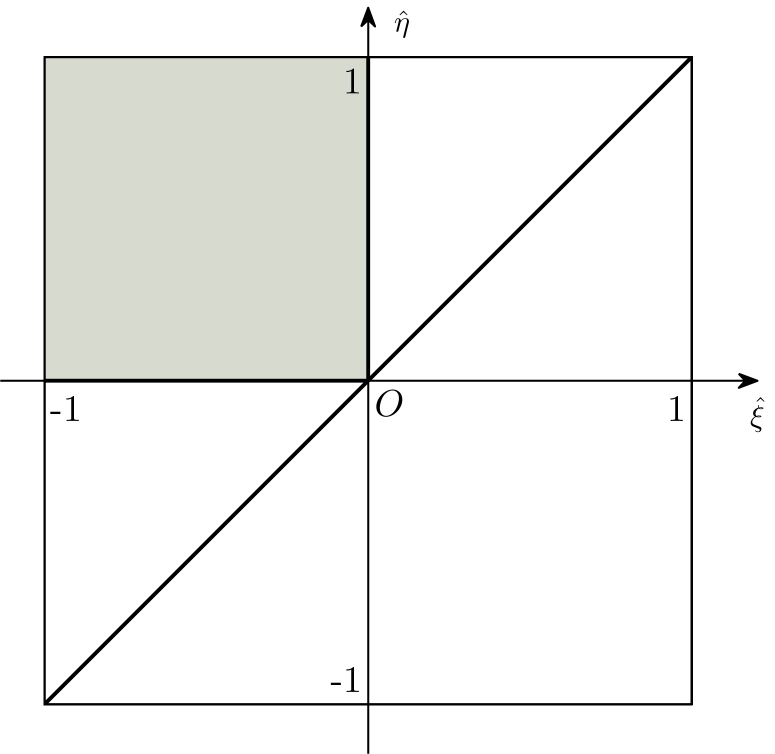
(a)

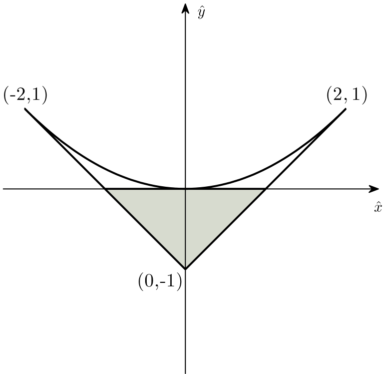
(b)

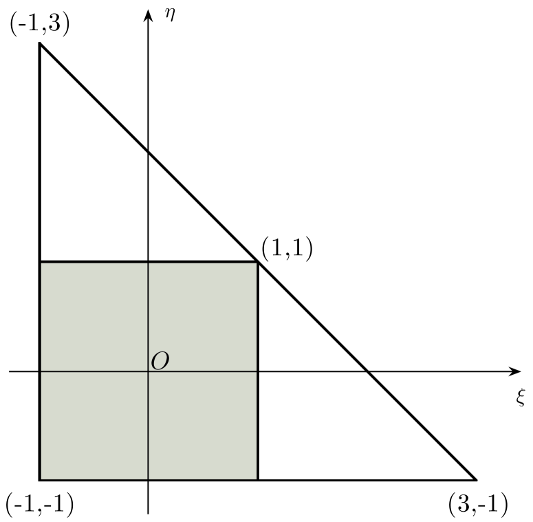
(c)

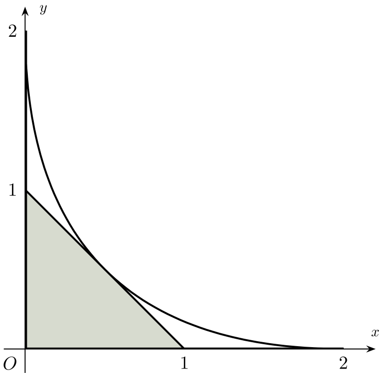
(d)

Figure 2.2. (a). The reference square ${\Box},$ the upper triangle ${\bigtriangleup}_{\mathrm{up}}=\left\{(x,y):-1<x<y<1\right\}$ and the square $\widehat{\Box}$ (shaded). (b). The image $\Omega$ (resp. $\widehat{\bigtriangleup}$ (shaded)) of the symmetric mapping $\widehat{T}$ whose domain is ${\bigtriangleup}_{\mathrm{up}}$ (resp. $\widehat{\Box}$ (shaded)). (c). Domains obtained from $\widehat{\Box}$ and the upper triangle ${\bigtriangleup}_{\mathrm{up}}$ in (a) by the affine mapping $F_{1}.$ (d). Domains obtained from $\widehat{\bigtriangleup}$ and $\Omega$ in (b) by the affine mapping $F_{2}.$

3. Basis functions and computation of the stiffness matrix

We introduce in this section the modal and nodal basis functions on triangles, and present a fast and accurate algorithm for computing the stiffness matrix with a focus on how to deal with the singularity (cf. (2.10)-(2.11)).

3.1. Modal basis

Observe from Lemma 2.1 and Remark LABEL:DuffyProp that for any polynomial $p$ on ${\bigtriangleup},$ its transformed counterpart $\tilde{p}$ remains a polynomial on ${\Box},$ but a general polynomial on ${\Box}$ is mapped to a rational or an irrational function on ${\bigtriangleup}$.

In order to obtain orthogonal polynomials on both ${\bigtriangleup}$ and ${\Box},$ Dubiner [10] introduced the polynomial basis using the Duffy’s transform (2.17):

$$\begin{split}D_{mn}(x,y)&=(1-y)^{m}J_{m}^{0,0}\Big{(}\frac{2x}{1-y}-1\Big{)}J^{2m+1,0}_{n}(2y-1)\\ &=J_{m}^{0,0}(\xi)\Big{(}\frac{1-\eta}{2}\Big{)}^{m}J^{2m+1,0}_{n}(\eta)=\tilde{D}_{mn}(\xi,\eta),\end{split}$$ (3.1)

Here, $J_{k}^{\alpha,\beta}(\zeta)$ $(\alpha,\beta>-1)$ are the Jacobi polynomials [32]. The so-defined $\{P_{mn}\}$ are orthogonal under the inner product (2.6). As the degree $m$ appears in the parameter of $J_{n}^{2m+1,0},$ this basis is not built upon a full tensor structure, which is called a warped tensor basis. The interested readers are referred to the monograph of Karniadakis and Sherwin [19] for a very extensive development of this notion. The error analysis of this approach can be found in [14, CHQZ, 22, 6].

By dropping the requirement of being polynomials on ${\bigtriangleup},$ Shen, Wang and Li [31] introduced fully tensorial rational basis functions based on the Duffy’s transform (2.17):

$$\begin{split}R_{mn}(x,y)&=J_{m}^{0,0}\Big{(}\frac{2x}{1-y}-1\Big{)}J^{1,0}_{n}(2y-1)=J_{m}^{0,0}(\xi)J^{1,0}_{n}(\eta)=\tilde{R}_{mn}(\xi,\eta),\end{split}$$ (3.2)

which are orthogonal with respect to $(\cdot,\cdot)_{{\bigtriangleup}}.$ This allows to the implementation as efficient as the rectangles (see further development in [CSX11]).

Let $I=(-1,1)$ as before. We define the space

$$Y_{N}({\bigtriangleup})={\mathcal{Q}}_{N}({\Box})\circ T^{-1}=(P_{N}(I))^{2}\circ T^{-1},$$ (3.3)

which consists of the images of the tensor-product polynomials on ${\Box}$ under the inverse mapping $T^{-1}$ defined in (2.2). As a direct consequence of Proposition 2.1 (ii), we have

$$Y_{N}({\bigtriangleup})={\mathcal{P}}_{N}({\bigtriangleup})\oplus\chi{\mathcal{P}}_{N-1}({\bigtriangleup}),$$ (3.4)

where $\chi=\sqrt{(x-y)^{2}+4(1-x-y)},$ and we recall that ${\mathcal{P}}_{N}({\bigtriangleup})$ is the set of polynomials on ${\bigtriangleup}$ of total degree at most $N.$ This implies that $Y_{N}({\bigtriangleup})$ contains not only polynomials, but also special irrational functions: $\chi\phi$ for any $\phi\in{\mathcal{P}}_{N-1}({\bigtriangleup}).$

Define

$$\begin{split}&\phi_{0}(\zeta)=\frac{1-\zeta}{2},\;\;\phi_{k}(\zeta)=\frac{1-\zeta^{2}}{4}J_{k-1}^{1,1}(\zeta),\;\;1\leq k\leq N-1,\;\;\phi_{N}(\zeta)=\frac{1+\zeta}{2},\end{split}$$ (3.5)

where $J_{k}^{1,1}$ is the Jacobi polynomial of degree $k$ (cf. [32]). It is clear that $\{\phi_{k}\}_{k=0}^{N}$ forms a basis of $P_{N}(I),$ and we have

$${\mathcal{Q}}_{N}({\Box})={\rm span}\big{\{}\Phi_{kl}:\Phi_{kl}(\xi,\eta)=\phi_{k}(\xi)\phi_{l}(\eta),\;0\leq k,l\leq N\big{\}}.$$ (3.6)

It is a commonly used $C^{0}$-modal basis for QSEM, which enjoys a distinct separation of the interior and boundary modes (including vertex and edge modes). All interior modes are zero on the triangle boundary. The vertex modes have a unit magnitude at one vertex and are zero at all other vertices, and the edge modes only have magnitude along one edge and are zero at all other vertices and edges.

In view of (3.3) and (3.6), we obtain the modal basis for $Y_{N}({\bigtriangleup}):$

$$Y_{N}({\bigtriangleup})={\rm span}\big{\{}\Psi_{kl}:\Psi_{kl}(x,y)=\Phi_{kl}\circ T^{-1},\;0\leq k,l\leq N\big{\}}.$$ (3.7)

3.2. Computation of the stiffness matrix

Though the singular integral of (2.11)-type has a finite value, some efforts are needed to compute such integrals in a fast and stable manner. Next, we devise an efficient algorithm for this purpose.

Let $L_{k}$ be the Legendre polynomial of degree $k,$ and recall that (see, e.g., [32])

$$(1-\zeta^{2})J_{k-1}^{1,1}(\zeta)=\frac{2k}{2k+1}\big{(}L_{k-1}(\zeta)-L_{k+1}(\zeta)\big{)},$$ (3.8)

$$(2k+1)L_{k}(\zeta)=L_{k+1}^{\prime}(\zeta)-L_{k-1}^{\prime}(\zeta),$$ (3.9)

$$\zeta L_{k}(\zeta)=\frac{k}{2k+1}L_{k-1}(\zeta)+\frac{k+1}{2k+1}L_{k+1}(\zeta).$$ (3.10)

Thus, we have

$$\phi_{0}^{\prime}(\zeta)=-\frac{1}{2}L_{0}(\zeta)=-\phi_{N}^{\prime}(\zeta),\quad\phi_{k}^{\prime}(\zeta)=-\frac{k}{2}L_{k}(\zeta),\;\;1\leq k\leq N-1.$$ (3.11)

By (2.5), (2.7) and (3.6),

$$\begin{split}&\chi\partial_{x}\Psi_{kl}=2\big{(}\phi_{k}^{\prime}(\xi)\phi_{l}(\eta)+\phi_{k}(\xi)\phi^{\prime}_{l}(\eta)\big{)}+\big{[}(1-\xi)\phi_{k}^{\prime}(\xi)\phi_{l}(\eta)-(1-\eta)\phi_{k}(\xi)\phi^{\prime}_{l}(\eta)\big{]},\\ &\chi\partial_{y}\Psi_{kl}=2\big{(}\phi_{k}^{\prime}(\xi)\phi_{l}(\eta)+\phi_{k}(\xi)\phi^{\prime}_{l}(\eta)\big{)}-\big{[}(1-\xi)\phi_{k}^{\prime}(\xi)\phi_{l}(\eta)-(1-\eta)\phi_{k}(\xi)\phi^{\prime}_{l}(\eta)\big{]}.\end{split}$$ (3.12)

Thanks to (3.8)-(3.11), $\chi\partial_{x}\Psi_{kl}$ and $\chi\partial_{y}\Psi_{kl}$ can be represented by a linear combination of $\{L_{k\pm i}(\xi)L_{l\pm j}(\eta)\}_{i,j=0,1}.$ In view of this, we can evaluate the entries of the stiffness matrix by computing the integrals of the product of Legendre polynomials:

$$s_{kl}^{k^{\prime}l^{\prime}}:=\int\int_{\bigtriangleup}\nabla\Psi_{kl}\cdot\nabla\Psi_{k^{\prime}l^{\prime}}\,\mathrm{d}x\mathrm{d}y\;\;\longleftrightarrow\;\;\int\int_{\Box}\frac{L_{i}(\xi)L_{j}(\eta)L_{i^{\prime}}(\xi)L_{j^{\prime}}(\eta)}{2-\xi-\eta}\,\mathrm{d}\xi\mathrm{d}\eta:=a_{ij}^{i^{\prime}j^{\prime}}.$$ (3.13)

Using the fact that the product $L_{m}L_{n}$ can be represented by $\{L_{p}\}_{p=0}^{m+n}$:

$$L_{m}(\xi)L_{n}(\xi)=\sum_{p=0}^{m+n}c_{p}^{mn}L_{p}(\xi),$$ (3.14)

where the expansion coefficient $\{c_{p}^{mn}\}$ can be found in e.g., [18], we obtain

$$a_{ij}^{i^{\prime}j^{\prime}}=\sum_{p=0}^{i+i^{\prime}}\sum_{q=0}^{j+j^{\prime}}c^{ii^{\prime}}_{p}c^{jj^{\prime}}_{q}\hat{a}_{pq},\;\;{\rm where}\;\;\hat{a}_{pq}=\int\int_{\Box}\frac{L_{p}(\xi)L_{q}(\eta)}{2-\xi-\eta}\,\mathrm{d}\xi\mathrm{d}\eta.$$ (3.15)

Now, we describe how to compute $\{\hat{a}_{pq}\}$ in a fast and accurate manner. This essentially relies on the following recurrence relation.

Lemma 3.1.

We have

$$\frac{\hat{a}_{p,q+1}-\hat{a}_{p,q-1}}{2q+1}=\frac{\hat{a}_{p+1,q}-\hat{a}_{p-1,q}}{2p+1},\quad\forall\,p,q\geq 1.$$ (3.16)

Proof.

The statement is true for $p=q\geq 1,$ since $\hat{a}_{p,p\pm 1}=\hat{a}_{p\pm 1,p}$. In view of the symmetry: $\hat{a}_{pq}=\hat{a}_{qp},$ it suffices to show it holds for $p\geq q\geq 1.$

We start with recalling the Legendre functions of the second kind (see, Formula (4.61.4) in [32]):

$$Q_{n}(x)=\frac{1}{2}\int_{-1}^{1}\frac{L_{n}(t)}{x-t}\,\mathrm{d}t,\quad n\geq 1;\quad Q_{0}(x)=\frac{1}{2}\ln\frac{x+1}{x-1},\quad\forall x>1,$$ (3.17)

and the important identity (see [32, Formula (4.62.1)]):

$$Q_{n}(x) =\frac{1}{2}\Big{(}\ln\frac{x+1}{x-1}\Big{)}L_{n}(x)-\frac{1}{2}\int_{-1}^{1}\frac{L_{n}(x)-L_{n}(t)}{x-t}\,\mathrm{d}t$$

$$=\frac{1}{2}\Big{(}\ln\frac{x+1}{x-1}\Big{)}L_{n}(x)-\tilde{L}_{n-1}(x).$$ (3.18)

Here, $\tilde{L}_{n}$ is the Legendre polynomial of the second kind, satisfying

$$\tilde{L}_{n}(x)=\frac{2n+1}{n+1}x\tilde{L}_{n-1}(x)-\frac{n}{n+1}\tilde{L}_{n-2}(x),\;\;n\geq 1;\quad\tilde{L}_{-1}(x)=0,\;\;\tilde{L}_{0}(x)=1,$$ (3.19)

which follows from (3.18) and [32, Formula (4.62.13)] directly.

Using (3.17)-(3.19) and the orthogonality of the Legendre polynomials, we find that for $p>q\geq 1$,

$$\hat{a}_{pq}= \int_{-1}^{1}\int_{-1}^{1}\frac{L_{p}(\xi)L_{q}(\eta)}{2-\xi-\eta}\,\mathrm{d}\xi\mathrm{d}\eta=2\int_{-1}^{1}Q_{q}(2-\xi)L_{p}(\xi)\,\mathrm{d}\xi$$

$$= \int_{-1}^{1}\Big{[}\Big{(}\ln\frac{3-\xi}{1-\xi}\Big{)}L_{q}(2-\xi)-2\tilde{L}_{q-1}(2-\xi)\Big{]}L_{p}(\xi)\,\mathrm{d}\xi$$

$$= \int_{-1}^{1}\Big{(}\ln\frac{3-\xi}{1-\xi}\Big{)}L_{q}(2-\xi)L_{p}(\xi)\,\mathrm{d}\xi.$$ (3.20)

Thus, we have from (3.9) and integration by parts that

$$\frac{\hat{a}_{p,q+1}-\hat{a}_{p,q-1}}{2q+1}=\int_{-1}^{1}\Big{(}\ln\frac{3-\xi}{1-\xi}\Big{)}\frac{L_{q+1}(2-\xi)-L_{q-1}(2-\xi)}{2q+1}L_{p}(\xi)\,\mathrm{d}\xi$$

$$\qquad=\int_{-1}^{1}\Big{(}\ln\frac{3-\xi}{1-\xi}\Big{)}\frac{L_{q+1}(2-\xi)-L_{q-1}(2-\xi)}{2q+1}\Big{[}\frac{L_{p+1}(\xi)-L_{p-1}(\xi)}{2p+1}\Big{]}^{\prime}\,\mathrm{d}\xi$$

$$\qquad=-\int_{-1}^{1}\left[\Big{(}\ln\frac{3-\xi}{1-\xi}\Big{)}\frac{L_{q+1}(2-\xi)-L_{q-1}(2-\xi)}{2q+1}\right]^{\prime}\frac{L_{p+1}(\xi)-L_{p-1}(\xi)}{2p+1}\,\mathrm{d}\xi.$$

Working out the derivative, we obtain

$$\frac{\hat{a}_{p,q+1}-\hat{a}_{p,q-1}}{2q+1}$$

$$\overset{(\ref{deriv})}{=}\int_{-1}^{1}\left[L_{q}(2-\xi)\ln\Big{(}\frac{3-\xi}{1-\xi}\Big{)}-\frac{L_{q+1}(2-\xi)-L_{q-1}(2-\xi)}{(q+1/2)(3-\xi)(1-\xi)}\right]\frac{L_{p+1}(\xi)-L_{p-1}(\xi)}{2p+1}\,\mathrm{d}\xi$$

$$\overset{(\ref{defncmb})}{=}\frac{\hat{a}_{p+1,q}-\hat{a}_{p-1,q}}{2p+1}-\int_{-1}^{1}\frac{L_{q+1}(2-\xi)-L_{q-1}(2-\xi)}{(q+1/2)(3-\xi)(1-\xi)}\frac{L_{p+1}(\xi)-L_{p-1}(\xi)}{2p+1}\,\mathrm{d}\xi$$

$$\overset{(\ref{Jacorec})}{=}\frac{\hat{a}_{p+1,q}-\hat{a}_{p-1,q}}{2p+1}+\frac{1}{2pq}\int_{-1}^{1}J^{1,1}_{q-1}(2-\xi)J^{1,1}_{p-1}(\xi)(1-\xi^{2})\,\mathrm{d}\xi$$

$$~{}~{}=\frac{\hat{a}_{p+1,q}-\hat{a}_{p-1,q}}{2p+1},$$

where we used the fact $p>q$ and the orthogonality of Jacobi polynomials in the last step.  

Equipped with (3.16), we are able to compute $\{\hat{a}_{pq}\}_{p\geq q}$ accurately and rapidly. We summarize the algorithm as follows.   Algorithm for computing $\{\hat{a}_{pq}\}_{p,q=0}^{N}$

• Initialization

  • For $p=0,1,\cdots,2N,$ compute $\hat{a}_{p0}\,;$

  • For $p=1,2,\cdots,2N-1,$ compute $\hat{a}_{p1}\,.$

• For $q=2,3,\cdots,N,$
  For $p=q,\cdots,2N-q,$

  $$\hat{a}_{pq}=\hat{a}_{p,q-2}+\frac{2q-1}{2p+1}({\hat{a}_{p+1,q-1}-\hat{a}_{p-1,q-1}}),$$ (3.21)

  Endfor of $p,q.$

• Set $\hat{a}_{pq}=\hat{a}_{qp}$ for all $0\leq p<q<N.$

 

We describe below the details for computing the initial values.

• We find from (3.20) that

  $$\hat{a}_{p0} =\int_{-1}^{1}L_{p}(\xi)\ln\frac{3-\xi}{1-\xi}\,\mathrm{d}\xi$$

  $$=\int_{-1}^{1}L_{p}(\xi)\ln\frac{3-\xi}{2}\,\mathrm{d}\xi+\int_{-1}^{1}L_{p}(\xi)\ln\frac{2}{1-\xi}\,\mathrm{d}\xi:=\alpha_{p}+\beta_{p}.$$ (3.22)

  It is clear that by (3.9) and integration by parts,

  $$\alpha_{p} =\int_{-1}^{1}L_{p}(\xi)\ln\frac{3-\xi}{2}\,\mathrm{d}\xi=\frac{1}{2p+1}\Big{(}\int_{-1}^{1}\frac{L_{p+1}(\xi)}{3-\xi}\,\mathrm{d}\xi-\int_{-1}^{1}\frac{L_{p-1}(\xi)}{3-\xi}\,\mathrm{d}\xi\Big{)}.$$

  It decays exponentially with respect to $p,$ and the use of a Legendre-Gauss quadrature leads to an exponentially accurate approximation, since the function $1/(3-\xi)$ is analytic within an ellipse (see [35]). We find from e.g., [12] that

  $$\beta_{p}=\int_{-1}^{1}L_{p}(\xi)\ln\frac{2}{1-\xi}\,\mathrm{d}\xi=\begin{cases}2,\quad&{\rm if}\;\;p=0,\\ \dfrac{2}{p(p+1)},\quad&{\rm if}\;\;p\geq 1.\end{cases}$$

• Using (3.15), (3.10) and the orthogonality of Legendre polynomials, we find

  $$\hat{a}_{p1} =\int\int_{\Box}\frac{\eta L_{p}(\xi)}{2-\xi-\eta}\,\mathrm{d}\xi\mathrm{d}\eta=\int\int_{\Box}\frac{(2-\xi)L_{p}(\xi)}{2-\xi-\eta}\,\mathrm{d}\xi\mathrm{d}\eta-\int\int_{\Box}\frac{(2-\xi-\eta)L_{p}(\xi)}{2-\xi-\eta}\mathrm{d}\xi\mathrm{d}\eta$$

  $$=2\int\int_{\Box}\frac{L_{p}(\xi)}{2-\xi-\eta}\,\mathrm{d}\xi\mathrm{d}\eta-\int\int_{\Box}\frac{\xi L_{p}(\xi)}{2-\xi-\eta}\,\mathrm{d}\xi\mathrm{d}\eta-\int_{-1}^{1}\left[\int_{-1}^{1}L_{p}(\xi)\,\mathrm{d}\xi\right]\mathrm{d}\eta$$

  $$=2\hat{a}_{p0}-\frac{(p+1)\hat{a}_{p+1,0}+p\hat{a}_{p-1,0}}{2p+1},\quad p\geq 1.$$ (3.23)

• We see that with an accurate computation of the initial values $\{\hat{a}_{p0}\}$, marching by (3.23) and (3.21) is expected to be stable. In Figure 3.1, we provide a schematic illustration of sweeping the stencils by the algorithm.

  

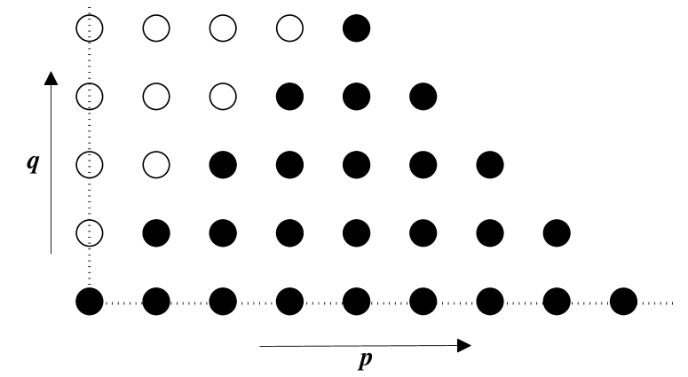
  Figure 3.1. Diagram for computing $\{\hat{a}_{pq}\}_{p,q=0}^{N}$ with $N=2,$ where the stencils marked by “$\bullet$” are marched via Steps 1-2 in the Algorithm, and those marked by “$\circ$” are obtained by the symmetric property in Step 3.

Remark 3.1.

We see that the rectangle-triangle mapping (2.1) essentially induces logarithmic singularity. Indeed, numerical quadrature of integrands involving a logarithmic weight function is of independent interest (see, e.g., [12]).  

Remark 3.2.

As a quick note, the mass matrix under this basis is sparse. Indeed, by (2.6),

$$(u,v)_{{\bigtriangleup}}=\frac{1}{8}\int\int_{\Box}\tilde{u}\tilde{v}\,\mathrm{d}\xi\mathrm{d}\eta-\frac{1}{16}\int\int_{\Box}\xi\tilde{u}\tilde{v}\,\mathrm{d}\xi\mathrm{d}\eta-\frac{1}{16}\int\int_{\Box}\eta\tilde{u}\tilde{v}\,\mathrm{d}\xi\mathrm{d}\eta,$$ (3.24)

so we claim this from (3.10) and the orthogonality of the Legendre polynomials.  

Remark 3.3.

With an additional affine mapping, any triangular element ${\bigtriangleup}_{\rm any}$ can be transformed to the reference square ${\Box}.$ It is important to point out that the stiffness and mass matrices on ${\bigtriangleup}_{\rm any}$ can be precomputed in a similar fashion as above. To justify this, we consider a general triangle ${\bigtriangleup}_{\rm any}$ with vertices $V_{i}=(x_{i},y_{i})$, $i=1,2,3$. Like (2.1), we have the mapping from ${\Box}$ to ${\bigtriangleup}_{\rm any}:$

$$(x,y)=(x_{1},y_{1})\frac{(1-\xi)(1-\eta)}{4}+(x_{2},y_{2})\frac{(1+\xi)(3-\eta)}{8}+(x_{3},y_{3})\frac{(3-\xi)(1+\eta)}{8},$$ (3.25)

for all $(\xi,\eta)\in{{\Box}}.$ A direct calculation leads to

$$\left(u,v\right)_{{\bigtriangleup}_{\rm any}}=\frac{F}{8}\int\int_{\Box}\tilde{u}\tilde{v}\,\mathrm{d}\xi\mathrm{d}\eta-\frac{F}{16}\int\int_{\Box}\xi\tilde{u}\tilde{v}\,\mathrm{d}\xi\mathrm{d}\eta-\frac{F}{16}\int\int_{\Box}\eta\tilde{u}\tilde{v}\,\mathrm{d}\xi\mathrm{d}\eta,$$ (3.26)

and

$$\left(\nabla u,\nabla v\right)_{{\bigtriangleup}_{\rm any}} =A\int\int_{\Box}\big{(}\widetilde{\nabla}\cdot\tilde{u}\big{)}\big{(}\widetilde{\nabla}\cdot\tilde{v}\big{)}\chi^{-1}\mathrm{d}\xi\mathrm{d}\eta+C\int\int_{\Box}\big{(}\widetilde{\nabla}^{\intercal}\tilde{u}\big{)}\big{(}\widetilde{\nabla}^{\intercal}\tilde{v}\big{)}\chi^{-1}\mathrm{d}\xi\mathrm{d}\eta$$

$$-B\int\int_{\Box}\big{[}\big{(}\widetilde{\nabla}\cdot\tilde{u}\big{)}(\widetilde{\nabla}^{\intercal}\tilde{v}\big{)}+\big{(}\widetilde{\nabla}^{\intercal}\tilde{u}\big{)}\big{(}\widetilde{\nabla}\cdot\tilde{v}\big{)}\big{]}\chi^{-1}\mathrm{d}\xi\mathrm{d}\eta,$$ (3.27)

where $\chi^{-1}=2/(2-\xi-\eta),$ the differential operators are defined in (2.5), and the constants are given by

$$F =(x_{2}-x_{1})(y_{3}-y_{1})-(x_{3}-x_{1})(y_{2}-y_{1})\not=0,$$

$$A =((x_{2}-x_{3})^{2}+(y_{2}-y_{3})^{2})/(2F),$$

$$B =((x_{2}-x_{1})^{2}+(y_{2}-y_{1})^{2}-(x_{3}-x_{1})^{2}-(y_{3}-y_{1})^{2})/(4F),$$

$$C =((2x_{1}-x_{2}-x_{3})^{2}+(2y_{1}-y_{2}-y_{3})^{2})/(8F).$$

In particular, if ${\bigtriangleup}_{\rm any}={\bigtriangleup},$ (3.26) and (3.27) (note: $B=0$) reduce to (2.6) and (2.8), respectively.

As with (3.12), we find from (3.8)-(3.11) that $\widetilde{\nabla}\cdot\Phi_{kl}$ and $\widetilde{\nabla}^{\intercal}\Phi_{kl}$ can be expressed in terms of $\{L_{k\pm i}(\xi)L_{l\pm j}(\eta)\}_{i,j=0,1},$ so the mass matrix on ${\bigtriangleup}_{\rm any}$ can be precomputed by the same algorithm described above.  

3.3. Interpolation, quadrature and nodal basis

Through the general mapping (3.25), the operations (e.g., interpolation, quadrature and numerical differentiations) on a triangular element can be performed on the reference square ${\Box}.$

Hereafter, let $\{\zeta_{j}\}_{j=0}^{N}$ be the Legendre-Gauss-Lobatto (LGL) points, i.e., the zeros of $(1-\zeta^{2})L^{\prime}_{N}(\zeta),$ and let $\{h_{j}\}_{j=0}^{N}$ be the associated Lagrangian basis polynomials such that $h_{j}\in P_{N}(I)$ and $h_{j}(\zeta_{k})=\delta_{kj},$ where $\delta_{kj}$ is the Kronecker delta. Given $v\in C(\bar{I}),$ the one-dimensional polynomial interpolant of $u$ is

$$(I_{N}^{\zeta}v)(\zeta)=\sum_{j=0}^{N}v(\zeta_{j})h_{j}(\zeta)\in P_{N},\quad\forall\,\zeta\in\bar{I}.$$ (3.28)

Recall that the LGL quadrature has the exactness:

$$\int_{-1}^{1}\phi(\zeta)d\zeta=\sum_{j=0}^{N}\phi(\zeta_{j})\omega_{j},\quad\forall\,\phi\in P_{2N-1}(I),$$ (3.29)

where $\{\omega_{j}\}$ are the LGL quadrature weights.

Given any $u\in C(\bar{\bigtriangleup}),$ we define the interpolant of $u$ by

$$(\operatorname{I\!I}_{N}u)(x,y)=(I_{N}^{\xi}I_{N}^{\eta}\tilde{u})\circ T^{-1}=\Big{(}\sum_{i,j=0}^{n}(u\circ T)(\xi_{i},\eta_{j})h_{i}(\xi)h_{j}(\eta)\Big{)}\circ T^{-1},$$ (3.30)

where $T$ and $T^{-1}$ are defined in (2.1) and (2.2) as before, and $\{\xi_{k}=\eta_{k}=\zeta_{k}\}_{k=0}^{N}$. Notice that $\operatorname{I\!I}_{N}u\in Y_{N}({\bigtriangleup}).$

We also extend the LGL quadrature to define the discrete inner product on ${\bigtriangleup}$ as

$$\langle u,v\rangle_{N,{\bigtriangleup}}=\frac{1}{8}\sum_{i,j=0}^{N}\tilde{u}(\xi_{i},\eta_{j})\tilde{v}(\xi_{i},\eta_{j})\chi(\xi_{i},\eta_{j})\omega_{i}\omega_{j},$$ (3.31)

where $\chi=(2-\xi-\eta)/2.$ As a consequence of (2.6), (3.29) and (3.3)-(3.4), there holds

$$\langle u,v\rangle_{N,{\bigtriangleup}}=(u,v)_{{\bigtriangleup}},\quad\forall\,u\cdot v\in Y_{2N-2}({\bigtriangleup}),$$ (3.32)

which also holds for all $u\cdot v\in{\mathcal{P}}_{2N-2}({\bigtriangleup}).$

Since $\{h_{k}h_{l}\}_{k,l=0}^{N}$ forms the nodal basis for ${\mathcal{Q}}_{N}({\Box}),$ we can obtain the nodal basis for $Y_{N}({\bigtriangleup}):$

$$Y_{N}({\bigtriangleup})={\rm span}\big{\{}\widehat{\Psi}_{kl}:\widehat{\Psi}_{kl}(x,y)=(h_{k}h_{l})\circ T^{-1}\,:\,0\leq k,l\leq N\big{\}}.$$ (3.33)

In view of (3.24), the mass matrix under this nodal basis can be computed easily as usual by tensorial LGL quadrature. However, the direct evaluation of the stiffness matrix like (3.13) is prohibitive, as there is no recursive way for the computation. In order to surmount this obstacle, we resort to the notion of “discrete transform” (cf. [30]). Like (3.12), we have

$$\begin{split}&\chi\partial_{x}\widehat{\Psi}_{kl}=2(h_{k}^{\prime}(\xi)h_{l}(\eta)+h_{k}(\xi)h^{\prime}_{l}(\eta))+[(1-\xi)h_{k}^{\prime}(\xi)h_{l}(\eta)-(1-\eta)h_{k}(\xi)h^{\prime}_{l}(\eta)]\in{\mathcal{Q}}_{N}({\Box}),\\ &\chi\partial_{y}\widehat{\Psi}_{kl}=2(h_{k}^{\prime}(\xi)h_{l}(\eta)+h_{k}(\xi)h^{\prime}_{l}(\eta))-[(1-\xi)h_{k}^{\prime}(\xi)h_{l}(\eta)-(1-\eta)h_{k}(\xi)h^{\prime}_{l}(\eta)]\in{\mathcal{Q}}_{N}({\Box}).\end{split}$$

The idea is to transform $\{\chi\partial_{x}\widehat{\Psi}_{kl}\}_{k,l=0}^{N}$ and $\{\chi\partial_{y}\widehat{\Psi}_{kl}\}_{k,l=0}^{N}$ to $\{L_{i}(\xi)L_{j}(\eta)\}_{i,j=0}^{N}$ via a two-dimensional discrete transform. Then the evaluation boils down to finding $\{a_{ij}^{i^{\prime}j^{\prime}}\}$ in (3.13) as before.

4. Estimates of orthogonal projection and interpolation errors

The section is devoted to error estimates of orthogonal projections and interpolations on triangles. These results will be essential for understanding the approximability of the basis functions, and provide important tools for error analysis of the TSEM for PDEs.

4.1. Orthogonal projections

We start with considering the projection $\Pi_{N}:L^{2}\!\left({\bigtriangleup}\right)\to Y_{N}({\bigtriangleup}),$ defined by

$$\big{(}\Pi_{N}u-u,v\big{)}_{\bigtriangleup}=0,\quad\forall\,v\in Y_{N}({\bigtriangleup}).$$ (4.1)

Theorem 4.1.

For any $u\in H^{r}({\bigtriangleup})$ with $r\geq 0$, we have

$$\|\Pi_{N}u-u\|_{{\bigtriangleup}}\leq cN^{-r}|u|_{r,{\bigtriangleup}},$$ (4.2)

where $c$ is a positive constant independent of $N$ and $u.$

Proof.

We have

$$\|\Pi_{N}u-u\|_{{\bigtriangleup}}\overset{(\ref{l2prj})}{=}\inf_{\phi\in Y_{N}({\bigtriangleup})}\|\phi-u\|_{{\bigtriangleup}}\overset{(\ref{Ynsps2})}{\leq}\|\psi-u\|_{{\bigtriangleup}},\quad\forall\psi\in{\mathcal{P}}_{N}({\bigtriangleup}).$$ (4.3)

Now, we take $\psi$ to be the best $L^{2}$-approximation in ${\mathcal{P}}_{N}({\bigtriangleup}),$ denoted by $\pi_{N}u.$ By [22, Theorem 3.3],

$$\|\pi_{N}u-u\|_{{\bigtriangleup}}\leq cN^{-r}\Big{(}\sum_{k_{1}+k_{2}+k_{3}=r}\big{\|}\partial_{x}^{k_{1}}\partial_{y}^{k_{2}}(\partial_{y}-\partial_{x})^{k_{3}}u\big{\|}^{2}_{\omega^{k_{1},k_{2},k_{3}},{\bigtriangleup}}\Big{)}^{1/2}\leq cN^{-r}|u|_{r,{\bigtriangleup}},$$ (4.4)

where $\omega^{k_{1},k_{2},k_{3}}=x^{k_{1}+k_{3}}y^{k_{2}+k_{3}}(1-x-y)^{k_{1}+k_{2}}$ is a Jacobi weight function on ${\bigtriangleup}.$ Therefore, the estimate (4.2) follows from (4.3) and (4.4).  

We now turn to the $H^{1}$-projection: $\Pi_{N}^{1}:H^{1}({\bigtriangleup})\to Y_{N}({\bigtriangleup})$ such that

$$\big{(}\nabla(\Pi_{N}^{1}u-u),\nabla v\big{)}_{{\bigtriangleup}}+\big{(}\Pi_{N}^{1}u-u,v\big{)}_{\bigtriangleup}=0,\quad\forall\,v\in Y_{N}({\bigtriangleup}),$$ (4.5)

and the $H^{1}_{0}$-projection: $\Pi_{N}^{1,0}:H^{1}_{0}({\bigtriangleup})\to Y_{N}^{0}({\bigtriangleup})=Y_{N}({\bigtriangleup})\cap H^{1}_{0}({\bigtriangleup}),$ defined by

$$\big{(}\nabla(\Pi_{N}^{1,0}u-u),\nabla v\big{)}_{{\bigtriangleup}}=0,\quad\forall\,v\in Y_{N}^{0}({\bigtriangleup}),$$ (4.6)

where $H^{1}_{0}({\bigtriangleup})$ is defined as usual, i.e., the subspace of $H^{1}({\bigtriangleup})$ with functions vanishing on the boundary of ${\bigtriangleup}.$

Theorem 4.2.

For any $u\in H^{1}_{0}({\bigtriangleup})\cap H^{r}({\bigtriangleup})$ with $r\geq 1$, we have

$$\|\Pi_{N}^{1,0}u-u\|_{\mu,{\bigtriangleup}}\leq cN^{\mu-r}|u|_{r,{\bigtriangleup}},\quad\mu=0,1,$$ (4.7)

where $c$ is a positive constant independent of $u$ and $N.$ It also holds for any $u\in H^{r}({\bigtriangleup})$ with $\Pi_{N}^{1}u$ in place of $\Pi_{N}^{1,0}u.$

Proof.

Here, we only provide the proof for the projector $\Pi_{N}^{1,0},$ as the estimate for $\Pi_{N}^{1}$ can be obtained in a very similar fashion.

By the Poincaré inequality, we know that the semi-norm $|\cdot|_{1,{\bigtriangleup}}$ is a norm of $H^{1}_{0}({\bigtriangleup}).$ Hence, by the definition (4.6),

$$\|u-\Pi_{N}^{1,0}\|_{1,{\bigtriangleup}}\leq c|\phi-u|_{1,{\bigtriangleup}}\leq c\|\phi-u\|_{1,{\bigtriangleup}},\quad\forall\,\phi\in Y_{N}({\bigtriangleup}).$$ (4.8)

It is known from (3.4) that ${\mathcal{P}}_{N}({\bigtriangleup})\subset Y_{N}({\bigtriangleup}),$ so we can take $\phi$ to be the orthogonal projection $\pi_{N}^{1,0}:H^{1}_{0}({\bigtriangleup})\to{\mathcal{P}}^{0}_{N}({\bigtriangleup})={\mathcal{P}}_{N}({\bigtriangleup})\cap H^{1}_{0}({\bigtriangleup}),$ defined by

$$\big{(}\nabla(\pi_{N}^{1,0}u-u),\nabla v\big{)}_{{\bigtriangleup}}=0,\quad\forall\,v\in{\mathcal{P}}_{N}^{0}({\bigtriangleup}).$$ (4.9)

We quote the estimate in [22, Theorem 3.4]:

$$\begin{split}\|\pi_{N}^{1,0}u-u\|_{1,{\bigtriangleup}}&\leq cN^{1-r}\Big{(}\sum_{k_{1}+k_{2}+k_{3}=r}\big{\|}\partial_{x}^{k_{1}}\partial_{y}^{k_{2}}(\partial_{y}-\partial_{x})^{k_{3}}u\big{\|}^{2}_{\omega^{k_{1},k_{2},k_{3}}_{+},{\bigtriangleup}}\Big{)}^{1/2}\\ &\leq cN^{1-r}|u|_{r,{\bigtriangleup}},\end{split}$$ (4.10)

where

$$\omega^{k_{1},k_{2},k_{3}}_{+}=x^{\max(k_{1}+k_{3}-1,0)}y^{\max(k_{2}+k_{3}-1,0)}(1-x-y)^{\max(k_{1}+k_{2}-1,0)}.$$

Hence, the estimate (4.7) with $\mu=1$ follows from (4.8) and (4.10).

To show (4.7) with $\mu=0$, we use a duality argument as in [7], which we sketch below. Given $g\in L^{2}\!\left({\bigtriangleup}\right),$ we consider the auxiliary problem: Find $u_{g}\in H^{1}_{0}({\bigtriangleup})$ such that

$$a(u_{g},v):=(\nabla u_{g},\nabla v)_{\bigtriangleup}=(g,v)_{{\bigtriangleup}},\quad\forall\,v\in H^{1}_{0}({\bigtriangleup}).$$ (4.11)

By a standard argument, we can show that this problem has a unique solution with the regularity $\|u_{g}\|_{2,{\bigtriangleup}}\leq c\|g\|_{{\bigtriangleup}}.$

Now, taking $v=u-\Pi_{N}^{1,0}u$ into (4.11), we find from (4.6) and (4.7) with $\mu=1$ that

$$\big{|}(g,u-\Pi_{N}^{1,0}u)_{\bigtriangleup}\big{|} =\big{|}a(u_{g},u-\Pi_{N}^{1,0}u)\big{|}=\big{|}a(u_{g}-\Pi_{N}^{1,0}u_{g},u-\Pi_{N}^{1,0}u)\big{|}$$

$$\leq\big{|}u_{g}-\Pi_{N}^{1,0}u_{g}\big{|}_{1,{\bigtriangleup}}\big{|}u-\Pi_{N}^{1,0}u\big{|}_{1,{\bigtriangleup}}$$

$$\leq cN^{-r}|u_{g}|_{2,{\bigtriangleup}}|u|_{r,{\bigtriangleup}}\leq cN^{-r}\|g\|_{{\bigtriangleup}}|u|_{r,{\bigtriangleup}}.$$

Finally, we derive

$$\big{\|}u-\Pi_{N}^{1,0}u\big{\|}_{{\bigtriangleup}}=\sup_{0\neq g\in L^{2}\!\left({\bigtriangleup}\right)}\frac{\big{|}(g,u-\Pi_{N}^{1,0}u)_{\bigtriangleup}\big{|}}{\|g\|_{{\bigtriangleup}}}\leq cN^{-r}|u|_{r,{\bigtriangleup}}.$$

This completes the proof.  

Remark 4.1.

It is seen that benefited from the fact that ${\mathcal{P}}_{N}({\bigtriangleup})\subset Y_{N}({\bigtriangleup}),$ we are able to obtain the optimal error estimates directly from the available polynomial approximation results on triangles.  

4.2. Estimation of interpolation error

Now, we estimate the error of interpolation by (3.30) on ${\bigtriangleup}$. The estimate of the one-dimensional LGL interpolation (cf. (3.28)) is useful for our analysis (see [30, Theorem 3.44]), that is, for any $v\in H^{r}(I)$ with $r\geq 1,$ we have

$$\big{\|}I_{N}^{\zeta}v-v\big{\|}_{L^{2}(I)}\leq cN^{-r}\big{\|}(1-\zeta^{2})^{(r-1)/2}v^{(r)}\big{\|}_{L^{2}(I)}.$$ (4.12)

Theorem 4.3.

For any $u\in H^{r}({\bigtriangleup})$ with $r\geq 2$,

$$\|\operatorname{I\!I}_{N}u-u\|_{{\bigtriangleup}}\leq cN^{-r}B_{r}(u),$$ (4.13)

where

$$B_{r}(u)=\begin{cases}|u|_{2,{\bigtriangleup}}+\|(\partial_{y}-\partial_{x})^{2}u\|_{J^{-1},{\bigtriangleup}}+\|\nabla\cdot u\|_{J^{-1},{\bigtriangleup}},\quad&{\rm if}\;\;r=2,\\ |u|_{r,{\bigtriangleup}}+|u|_{r-1,{\bigtriangleup}},\quad&{\rm if}\;\;r\geq 3,\end{cases}$$ (4.14)

$J$ is the Jacobian as defined in (2.4), and $c$ is a constant independent of $u$ and $N$.

Proof.

To this end, let ${I_{d}}$ be the identity operator. Using (2.6), (3.30) and (4.12), we obtain

$$\big{\|}\operatorname{I\!I}_{N}u-u\big{\|}_{{\bigtriangleup}} \leq c\big{\|}I_{N}^{\xi}I_{N}^{\eta}\tilde{u}-\tilde{u}\big{\|}_{{\Box}}=c\big{\|}(I_{N}^{\xi}-I_{d})(I_{N}^{\eta}-I_{d})\tilde{u}+(I_{N}^{\xi}-I_{d})\tilde{u}+(I_{N}^{\eta}-I_{d})\tilde{u}\big{\|}_{{\Box}}$$

$$\leq c\big{(}\big{\|}(I_{N}^{\xi}-I_{d})(I_{N}^{\eta}-I_{d})\tilde{u}\big{\|}_{{\Box}}+\big{\|}(I_{N}^{\xi}-I_{d})\tilde{u}\big{\|}_{{\Box}}+\big{\|}(I_{N}^{\eta}-I_{d})\tilde{u}\big{\|}_{{\Box}}\big{)}$$

$$\leq cN^{-1}\big{\|}(I_{N}^{\eta}-I_{d})\partial_{\xi}\tilde{u}\big{\|}_{{\Box}}+c\big{(}\big{\|}(I_{N}^{\xi}-I_{d})\tilde{u}\big{\|}_{{\Box}}+\big{\|}(I_{N}^{\eta}-I_{d})\tilde{u}\big{\|}_{{\Box}}\big{)}$$

$$\leq cN^{-r}\big{(}\big{\|}(1-\eta^{2})^{(r-2)/2}\partial_{\xi}\partial_{\eta}^{r-1}\tilde{u}\big{\|}_{{\Box}}+\big{\|}(1-\xi^{2})^{(r-1)/2}\partial_{\xi}^{r}\tilde{u}\big{\|}_{{\Box}}$$

$$\qquad+\big{\|}(1-\eta^{2})^{(r-1)/2}\partial_{\eta}^{r}\tilde{u}\big{\|}_{{\Box}}\big{)}.$$

It remains to transform the variables $(\xi,\eta)$ back to $(x,y)$ and obtain tight upper bounds of the right-hand side using norms of $u$ on ${\bigtriangleup}$. By (2.3),

$$\partial_{\xi}\tilde{u} =\frac{1-\eta}{4}\partial_{y}u-\frac{3-\eta}{8}(\partial_{y}-\partial_{x})u=\frac{1-\eta}{4}\partial_{x}u-\frac{1+\eta}{8}(\partial_{y}-\partial_{x})u,$$ (4.15)

$$\partial_{\eta}\tilde{u} =\frac{1-\xi}{4}\partial_{x}u+\frac{3-\xi}{8}(\partial_{y}-\partial_{x})u=\frac{1-\xi}{4}\partial_{y}u+\frac{1+\xi}{8}(\partial_{y}-\partial_{x})u.$$ (4.16)

Thus, we have

$$\partial^{r}_{\xi}\tilde{u}=\sum\limits_{k=0}^{r}(-1)^{k}\binom{r}{k}\left(\frac{1+\eta}{8}\right)^{k}\left(\frac{1-\eta}{4}\right)^{r-k}\partial^{r-k}_{x}(\partial_{y}-\partial_{x})^{k}u,$$ (4.17)

and

$$\big{\|}(1-\xi^{2})^{(r-1)/2} \partial_{\xi}^{r}\tilde{u}\big{\|}_{{\Box}}^{2}=\int\int_{\Box}|\partial_{\xi}^{r}\tilde{u}|^{2}(1-\xi^{2})^{r-1}\mathrm{d}\xi\mathrm{d}\eta$$

$$\leq c\sum\limits_{k=0}^{r}\int\int_{\bigtriangleup}\big{|}\partial^{r-k}_{x}(\partial_{y}-\partial_{x})^{k}u\big{|}^{2}\frac{Q(\xi,\eta;r,k)}{J}\,\mathrm{d}x\mathrm{d}y,$$

where

$$Q(\xi,\eta;r,k)=\Big{(}\frac{1+\eta}{8}\Big{)}^{2k}\Big{(}\frac{1-\eta}{4}\Big{)}^{2r-2k}(1-\xi^{2})^{r-1}.$$

One verifies readily from (2.1) that

$$\frac{1}{4}(1-\xi)(1-\eta)=1-x-y,$$ (4.18)

$$\frac{1}{4}{(1+\xi)(1-\eta)}+\frac{1}{8}{(1+\xi)(1+\eta)}=x,$$ (4.19)

$$\frac{1}{4}{(1-\xi)(1+\eta)}+\frac{1}{8}{(1+\xi)(1+\eta)}=y.$$ (4.20)

Therefore, by (4.18)-(4.20), we derive that for $2\leq r\leq k-1,$

$$Q(\xi,\eta;r,k) =\frac{1}{2^{k}}\Big{[}(1+\xi)^{k}\Big{(}\frac{1+\eta}{8}\Big{)}^{k}\Big{]}\Big{[}(1-\xi)^{k}\Big{(}\frac{1+\eta}{4}\Big{)}^{k}\Big{]}$$

$$\quad\times\Big{(}\frac{(1+\xi)(1-\eta)}{4}\Big{)}^{r-k-1}\Big{(}\frac{(1-\xi)(1-\eta)}{4}\Big{)}^{r-k-1}\frac{(1-\eta)^{2}}{16}$$

$$\leq cx^{k}y^{k}x^{r-k-1}(1-x-y)^{r-k-1}J^{2}\leq c\varpi^{r-1,k,r-k-1}J,$$

where we used the fact: $1-\eta\leq 2-\xi-\eta=16J,$ and denoted by $\varpi^{\alpha,\beta,\gamma}=x^{\alpha}y^{\beta}(1-x-y)^{\gamma}.$ Similarly, for $2\leq r=k,$

$$Q(\xi,\eta;r,k) =\frac{1}{2^{r}}\Big{(}\frac{(1+\xi)(1+\eta)}{8}\Big{)}^{r-1}\Big{(}\frac{(1-\xi)(1+\eta)}{4}\Big{)}^{r-2}\Big{(}\frac{(1+\eta)}{4}\Big{)}^{2}(1-\xi)$$

$$\leq cx^{r-1}y^{r-2}J\leq c\varpi^{r-1,r-2,0}J,$$

where we used $1-\xi\leq 2-\xi-\eta=16J.$ Consequently, we obtain for $r\geq 2,$

$$\begin{split}&\big{\|}(1-\xi^{2})^{(r-1)/2}\partial_{\xi}^{r}\tilde{u}\big{\|}_{{\Box}}\\ &\quad\leq c\Big{(}\sum_{k=0}^{r-1}\big{\|}\partial_{x}^{r-k}(\partial_{y}-\partial_{x})^{k}u\big{\|}_{\varpi^{r-1,k,r-k-1},{\bigtriangleup}}^{2}+\big{\|}(\partial_{y}-\partial_{x})^{r}u\big{\|}_{\varpi^{r-1,r-2,0},{\bigtriangleup}}^{2}\Big{)}^{\frac{1}{2}}\\ &\quad\leq c\big{(}|u|_{r-1,{\bigtriangleup}}+|u|_{r,{\bigtriangleup}}\big{)}.\end{split}$$ (4.21)

By swapping $x\leftrightarrow y$ and $\xi\leftrightarrow\eta$, we get that for $r\geq 2,$

$$\big{\|}(1-\eta^{2})^{(r-1)/2}\partial_{\eta}^{r}\tilde{u}\big{\|}_{{\Box}}\leq c\big{(}|u|_{r-1,{\bigtriangleup}}+|u|_{r,{\bigtriangleup}}\big{)}.$$ (4.22)

We now turn to deal with the term $\big{\|}(1-\xi^{2})^{(r-2)/2}\partial_{\eta}\partial_{\xi}^{r-1}\tilde{u}\big{\|}_{{\Box}}$. By (4.16) and (4.17),

$$\partial_{\eta}\partial^{r-1}_{\xi}\tilde{u}=\partial_{\eta}\left[\sum\limits_{k=0}^{r-1}(-1)^{k}\binom{r-1}{k}\left(\frac{1+\eta}{8}\right)^{k}\left(\frac{1-\eta}{4}\right)^{r-k-1}\partial^{r-k-1}_{x}(\partial_{y}-\partial_{x})^{k}u\right]$$

$$\quad=\sum_{k=0}^{r}W_{1}(\xi,\eta;r,k)\partial^{r-k}_{x}(\partial_{y}-\partial_{x})^{k}u+\sum_{k=0}^{r-1}W_{2}(\xi,\eta;r,k)\partial^{r-k-1}_{x}(\partial_{y}-\partial_{x})^{k}u,$$ (4.23)

where $W_{1}$ and $W_{2}$ are polynomials of $\xi$ and $\eta.$ Thus, we have

$$\big{\|}(1-\xi^{2})^{(r-2)/2}\partial_{\eta}\partial_{\xi}^{r-1}\tilde{u}\big{\|}_{{\Box}}^{2} \leq c\sum_{k=0}^{r}\int\int_{\bigtriangleup}\left|\partial^{r-k}_{x}(\partial_{y}-\partial_{x})^{k}u\right|^{2}\frac{(1-\xi^{2})^{r-2}}{J}\,\mathrm{d}x\mathrm{d}y$$

$$+c\sum_{k=0}^{r-1}\int\int_{\bigtriangleup}\left|\partial^{r-k-1}_{x}(\partial_{y}-\partial_{x})^{k}u\right|^{2}\frac{(1-\xi^{2})^{r-2}}{J}\,\mathrm{d}x\mathrm{d}y.$$

This implies that for $r\geq 3,$

$$\big{\|}(1-\xi^{2})^{(r-2)/2}\partial_{\eta}\partial_{\xi}^{r-1}\tilde{u}\big{\|}_{{\Box}}\leq c\big{(}|u|_{r-1,{\bigtriangleup}}+|u|_{r,{\bigtriangleup}}\big{)}.$$ (4.24)

For $r=2,$ we obtain from a direct calculation that

$$\begin{split}\|\partial_{\xi}\partial_{\eta}\tilde{u}\|_{\Box}&\leq|u|_{2,{\bigtriangleup}}+\frac{1}{256}\|(\partial_{y}-\partial_{x})^{2}u\|_{J^{-1},{\bigtriangleup}}+\frac{1}{64}\|\nabla\cdot u\|_{J^{-1},{\bigtriangleup}}.\end{split}$$ (4.25)

A combination of (4.21)-(4.22) and (4.24)-(4.25) leads to the desired result.  

Remark 4.2.

Like (4.21), we could obtain sharper estimates with semi-norms in the upper bound of (4.13) featured with the Jacobi-type weight functions $\varpi^{\alpha,\beta,\gamma}.$

Notice that for $r=2,$ the semi-norms are weighted with $J^{-1},$ as we can not factor out $1-\xi$ or $1-\eta$ from $W_{1}$ and $W_{2}$ in (4.23) to eliminate $J^{-1}$. However, we point out that the value of $\int\int_{{\bigtriangleup}}J^{-1}\mathrm{d}x\mathrm{d}y$ is finite.  

5. Numerical results and concluding remarks

In this section, we just provide some numerical results to demonstrate the high accuracy of the proposed algorithm for model elliptic problems on ${\bigtriangleup}.$ We also intend to compare it with the standard tensor-product spectral approximations on rectangles to assess the performance of our approach.

Consider the elliptic equation:

$$\begin{split}&-\Delta u+\gamma u=f,\quad\text{ in }{\bigtriangleup}\,,\quad u|_{\Gamma_{1}}=0,\quad\frac{\partial u}{\partial\nu}\Big{|}_{\Gamma_{2}}=g,\end{split}$$ (5.1)

where the constant $\gamma\geq 0,$ $\Gamma_{1}$ is the edges $x=0$ and $y=0$, $\Gamma_{2}$ is the hypotenuse of ${\bigtriangleup},$ and ${\nu}$ is the unit vector outer normal to $\Gamma_{2}.$

5.1. The scheme and its convergence

A weak formulation of (5.1) is to find $u\in H^{1}_{\Gamma_{1}}({\bigtriangleup}):=\big{\{}u\in H^{1}({\bigtriangleup}):u|_{\Gamma_{1}}=0\big{\}}$ such that

$$\begin{split}&{\mathcal{B}}(u,v):=(\nabla u,\nabla v)_{{\bigtriangleup}}+\gamma(u,v)_{{\bigtriangleup}}=(f,v)_{{\bigtriangleup}}+\gamma\langle g,v\rangle_{\Gamma_{2}},\quad\forall\,v\in H^{1}_{\Gamma_{1}}({\bigtriangleup}),\end{split}$$ (5.2)

where $\langle\cdot,\cdot\rangle_{\Gamma_{2}}$ is the inner product of $L^{2}(\Gamma_{2}).$ It follows from a standard argument that if $f\in L^{2}({\bigtriangleup})$ and $g\in L^{2}(\Gamma_{2}),$ the problem (5.2) admits a unique solution in $H^{1}_{\Gamma_{1}}({\bigtriangleup})$.

The spectral-Galerkin approximation of (5.2) is to find $u_{N}\in Y_{N}^{\Gamma_{1}}({\bigtriangleup}):=Y_{N}({\bigtriangleup})\cap H^{1}_{\Gamma_{1}}({\bigtriangleup})$ such that for any $v_{N}\in Y_{N}^{\Gamma_{1}}({\bigtriangleup}),$

$${\mathcal{B}}_{N}(u_{N},v_{N}):=(\nabla u_{N},\nabla v_{N})_{{\bigtriangleup}}+\gamma(u_{N},v_{N})_{{\bigtriangleup}}=(\operatorname{I\!I}_{N}f,v_{N})_{{\bigtriangleup}}+\langle g,v_{N}\rangle_{N,\Gamma_{2}},$$ (5.3)

where $\operatorname{I\!I}_{N}$ is the interpolation operator as defined in (3.31), and the discrete inner product $\langle g,v_{N}\rangle_{N,\Gamma_{2}}$ can be defined on the quadrature rule:

$$\int_{\Gamma_{2}}g\,\mathrm{d}\gamma=\frac{\sqrt{2}}{2}\Big{[}\int_{-1}^{1}\tilde{g}(\xi,1)\mathrm{d}\xi-\int_{-1}^{1}\tilde{g}(1,\eta)\mathrm{d}\eta\Big{]}\sim\frac{1}{\sqrt{2}}\Big{[}\sum\limits_{j=0}^{N}\big{(}\tilde{g}(\zeta_{j},1)-\tilde{g}(1,\zeta_{j})\big{)}\omega_{j}\Big{]},$$ (5.4)

where $\{\zeta_{j},\omega_{j}\}$ are the LGL interpolation nodes and weights as before. More precisely, we define

$$\langle g,v_{N}\rangle_{N,\Gamma_{2}}=\frac{1}{\sqrt{2}}\sum_{j=0}^{N}\tilde{g}(\zeta_{j},1)\tilde{v}_{N}(\zeta_{j},1)\omega_{j}-\frac{1}{\sqrt{2}}\sum_{j=0}^{N}\tilde{g}(1,\zeta_{j})\tilde{v}_{N}(1,\zeta_{j})\omega_{j},$$ (5.5)

where $\tilde{g}=g\circ T$ and $\tilde{v}_{N}=v_{N}\circ T$.

Remark 5.1.

Here, we purposely impose the Neumann boundary condition on the hypotenuse of ${\bigtriangleup},$ so that the basis functions associated with this “singular” edge are involved in the computation.

We reiterate that a distinctive difference with the scheme in [24, Eqn. (25)] lies in that the consistency condition (2.9) is not needed to be built in the approximation space, which significantly facilitates the implementation. Note that the approaches based on the Duffy’s transform also need to modify the basis functions to meet the corresponding consistency condition (see, e.g., [31, 4]).  

To analyze the convergence of (5.3), it is essential to study the approximability of the orthogonal projection: $\Pi_{N}^{1,\Gamma_{1}}:H^{1}_{\Gamma_{1}}({\bigtriangleup})\to Y_{N}^{\Gamma_{1}}({\bigtriangleup}),$ such that

$$\big{(}\nabla(\Pi_{N}^{1,\Gamma_{1}}u-u),\nabla\phi)_{{\bigtriangleup}}=0,\quad\forall\phi\in Y_{N}^{\Gamma_{1}}({\bigtriangleup}).$$

Following the lines of the proof of Theorem 4.2, we find that (4.7) holds with $\Pi_{N}^{1,\Gamma_{1}}$ and $H^{1}_{\Gamma_{1}}({\bigtriangleup})$ in place of $\Pi_{N}^{1,0}$ and $H^{1}_{0}({\bigtriangleup})$, respectively.

Another ingredient for the analysis is to estimate the error between the continuous and discrete inner products on $\Gamma_{2}$. Using [30, Lemma 4.8] leads to

$$\big{|}\langle g,v_{N}\rangle_{N,\Gamma_{2}}-\langle g,v_{N}\rangle_{\Gamma_{2}}\big{|}\leq cN^{-t}\Big{(}\big{\|}(1-\xi^{2})^{(t-1)/2}\partial_{\xi}^{t}\tilde{g}(\cdot,1)\big{\|}_{L^{2}(I)}\|\tilde{v}_{N}(\cdot,1)\|_{L^{2}(I)}$$

$$+\big{\|}(1-\eta^{2})^{(t-1)/2}\partial_{\eta}^{t}\tilde{g}(1,\cdot)\big{\|}_{L^{2}(I)}\|\tilde{v}_{N}(1,\cdot)\|_{L^{2}(I)}\Big{)}.$$

Then we obtain from (4.15)-(4.16) and a derivation similar to the proof of Theorem 4.3 the following estimate:

$$\begin{split}\big{|}\langle g,v_{N}\rangle_{N,\Gamma_{2}}-\langle g,v_{N}\rangle_{\Gamma_{2}}\big{|}&\leq cN^{-t}\|(xy)^{(t-1)/2}(\partial_{y}-\partial_{x})^{t}g\|_{\Gamma_{2}}\|v_{N}\|_{\Gamma_{2}}\\ &\leq cN^{-t}|g|_{t,\Gamma_{2}}\|v_{N}\|_{\Gamma_{2}},\quad t\geq 1.\end{split}$$ (5.6)

With the above preparations, we can prove the convergence of the scheme (5.3) by using Theorems 4.2-4.3, the estimate (5.6) and a standard argument for error estimate of spectral approximation of elliptic problems.

Theorem 5.1.

Let $u$ and $u_{N}$ be the solutions of (5.2) and (5.3), respectively. If $u\in H^{1}_{\Gamma_{1}}({\bigtriangleup})\cap H^{r}({\bigtriangleup})$, $f\in H^{s}({\bigtriangleup})$ and $g\in H^{t}(\Gamma_{2})$ with $r\geq 1,s\geq 2$ and $t\geq 1$, then we have

$$\|u-u_{N}\|_{\mu,{\bigtriangleup}}\leq c\big{(}N^{\mu-r}|u|_{r,{\bigtriangleup}}+N^{-s}B_{s}(f)+N^{-t}|g|_{t,\Gamma_{2}}\big{)},$$

where $\mu=0,1,$ $B_{s}(f)$ is defined in (4.14), and $c$ is a positive constant independent of $N$ and $u,f,g.$

5.2. Numerical results

We first intend to show the typical spectral accuracy of the proposed method, so we particularly test it on (5.1) (with $\gamma=1$) with the exact solution:

$$u(x,y)=e^{x+y-1}\sin\big{(}3xy\big{(}y-{\sqrt{3}x}/{2}+{\sqrt{3}}/{4}\big{)}\big{)},\quad\forall\,(x,y)\in{\bigtriangleup}.$$ (5.7)

For comparison, we also consider the standard tensor polynomial approximation of (5.1) on a square $S=(0,1/\sqrt{2})^{2}$ (note: it has the same area as ${\bigtriangleup}$) under a similar setting, i.e., Neumann data on two edges $x=1/\sqrt{2}$ and $y=1/\sqrt{2},$ and homogeneous Dirichet data on the other two edges. We take the exact solution:

$$u(x,y)={\rm exp}\Big{(}-\Big{(}\frac{1}{\sqrt{2}}-x\Big{)}\Big{(}\frac{1}{\sqrt{2}}-y\Big{)}\Big{)}\sin\big{(}3xy\big{(}y-{\sqrt{3}x}/{2}+{\sqrt{3}}/{4}\big{)}\big{)},\quad\forall(x,y)\in S.$$ (5.8)

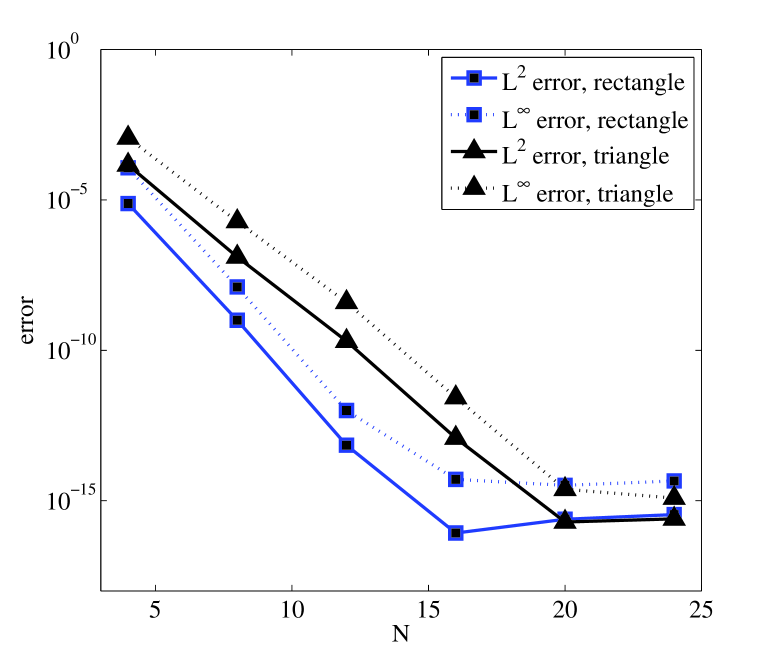
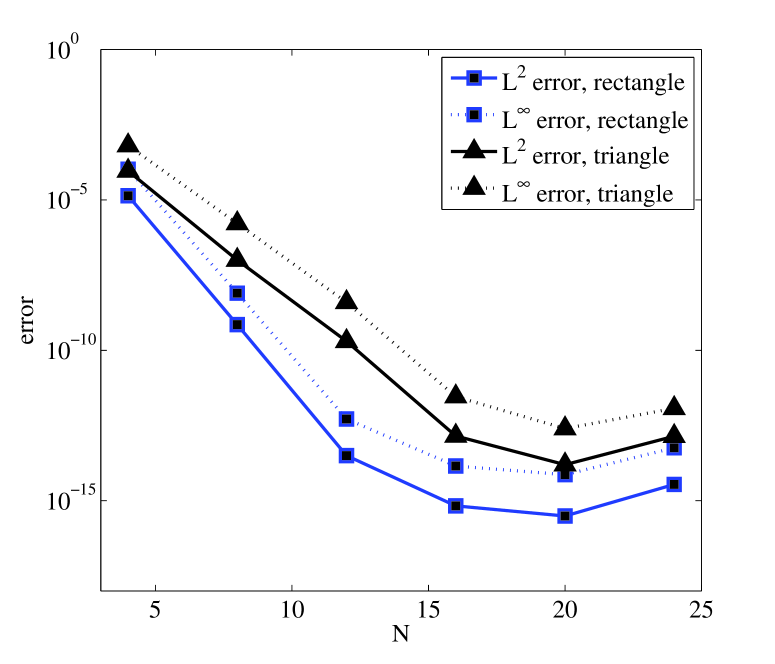
Figure 5.1. Numerical errors of (5.3) vs. tensorial polynomial approximation on the square $S$. Left: $L^{2}$- and $L^{\infty}$-errors using modal basis. Right: $L^{2}$- and $L^{\infty}$-errors using nodal basis.

In Figure 5.1, we plot the numerical errors of two methods, from which we observe that they share a very similar convergence behavior and the errors decay like $O(e^{-cN}).$ For a fixed $N,$ the accuracy of approximation on $S$ seems to be slightly better than expected. We refer to [3, Figure 2.17] for a similar comparison of the polynomial approximations on triangles [10] and rectangles. Indeed, the accuracy is comparable to the existing means in [19, 31, 24].

In the second test, we choose the exact solution of (5.1) with finite regularity:

$$u(x,y)=(1-x-y)^{\frac{5}{2}}(e^{xy}-1),\quad\forall\,(x,y)\in{\bigtriangleup},$$ (5.9)

which belongs to $H^{3-\epsilon}({\bigtriangleup})$ (for small $\epsilon>0$). The counterpart on the square $S$ takes the form:

$$u(x,y)=\Big{(}\frac{1}{\sqrt{2}}-x\Big{)}^{\frac{5}{2}}\Big{(}\frac{1}{\sqrt{2}}-y\Big{)}^{\frac{5}{2}}(e^{xy}-1),\quad\forall\,(x,y)\in S.$$ (5.10)

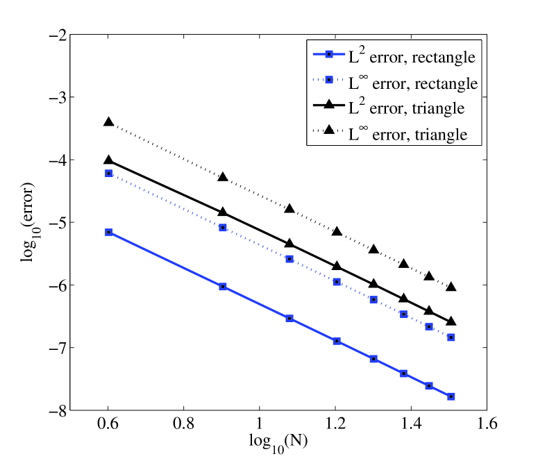
Figure 5.2. Numerical errors of (5.3) vs. tensorial polynomial approximation on the square $S$ with solutions having finite regualrity. Left: $L^{2}$- and $L^{\infty}$-errors using modal basis. Right: $L^{2}$- and $L^{\infty}$-errors using nodal basis.

We depict in Figure 5.2 the numerical errors of two approaches in $\log$-$\log$ scale, where the slopes of the lines are all roughly $-3$ as predicted by the theoretical results (cf. Theorem 5.1).

Table 5.1. Comparison between the approach in [24] and the new method

$N$	Approach in [24]		Approach in this paper
	$L^{2}$-error	$L^{\infty}$-error	$L^{2}$-error	$L^{\infty}$ error
15	$2.866E\mathrm{-}06$	$1.018E\mathrm{-}05$	$2.349E\mathrm{-}06$	$8.281E\mathrm{-}06$
30	$3.410E\mathrm{-}07$	$1.203E\mathrm{-}06$	$3.087E\mathrm{-}07$	$1.091E\mathrm{-}06$
45	$9.940E\mathrm{-}08$	$3.513E\mathrm{-}07$	$9.299E\mathrm{-}08$	$3.283E\mathrm{-}07$

Finally, we compare our new approach with the method in [24] (where the explicit consistency condition (2.9) was built in the approximation space). One can see from Table 5.1 that both approaches enjoy a similar convergence behavior. We reiterate that the new method does not require to modify the basis function, so with a pre-computation of the stiffness matrix, the triangular element can be treated as efficiently as the quadrilateral element.

5.3. Concluding remarks

We initiated in this paper a new TSEM through presenting the detailed implementation and analysis on a triangle. We demonstrated that the use of the rectangle-triangle mapping in [24] led to much favorable grid distributions, when compared with the commonly-used Duffy’s transform. More importantly, we showed the induced singularity could be fully removed. It is anticipated that with this initiative, we can develop an efficient TSEM on unstructured meshes built on a suitable discontinuous Galerkin formulation. This will be discussed in a forthcoming work.

References

- [1] R.A. Adams. Sobolov Spaces. Acadmic Press, New York, 1975.
- [2] J.P. Boyd and F. Yu. Comparing seven spectral methods for interpolation and for solving the Poisson equation in a disk: Zernike polynomials, Logan-Shepp ridge polynomials, Chebyshev-Fourier series, cylindrical Robert functions, Bessel-Fourier expansions, square-to-disk conformal mapping and radial basis functions. J. Comput. Phys., 230(4):1408–1438, 2011.
- [3] C. Canuto, M.Y. Hussaini, A. Quarteroni, and T.A. Zang. Spectral Methods. Scientific Computation. Springer, Berlin, 2007. Evolution to complex geometries and applications to fluid dynamics.
- [4] L. Chen, J. Shen, and C. Xu. A triangular spectral method for Stokes equations. Numer. Math.: Theory, Methods Appl., 4:158–179, 2011.
- [5] Q. Chen and I.M. Babuška. Approximate optimal points for polynomial interpolation of real functions in an interval and in a triangle. Comp. Meth. Appl. Math. Eng., 128(2):405–417, 1995.
- [6] A. Chernov. Optimal convergence estimates for the trace of the polynomial -projection operator on a simplex. Math. Comp., 81(278):765–787, 2011.
- [7] P.G. Ciarlet. The Finite Element Method for Elliptic Problems. North-Holland, 1978.
- [8] B. Cockburn, J. Gopalakrishnan, and R. Lazarov. Unified hybridization of discontinuous Galerkin, mixed, and continuous Galerkin methods for second order elliptic problems. SIAM J. Numer. Anal., 47(2):1319–1365, 2009.
- [9] M.O. Deville, P.F. Fischer, and E.H. Mund. High-Order Methods for Incompressible Fluid Flow, volume 9 of Cambridge Monographs on Applied and Computational Mathematics. Cambridge University Press, Cambridge, 2002.
- [10] M. Dubiner. Spectral methods on triangles and other domains. J. Sci. Comput., 6(4):345–390, 1991.
- [11] M.G. Duffy. Quadrature over a pyramid or cube of integrands with a singularity at a vertex. SIAM J. Numer. Anal., 19(6):1260–1262, 1982.
- [12] W. Gautschi. Gauss quadrature routines for two classes of logarithmic weight functions. Numer. Algorithms, 55(2-3):265–277, 2010.
- [13] W.J. Gordon and C.A. Hall. Construction of curvilinear co-ordinate systems and applications to mesh generation. Internat. J. Numer. Methods Engrg., 7:461–477, 1973.
- [14] B.Y. Guo and L. Wang. Error analysis of spectral method on a triangle. Adv. Comput. Math., 26(4):473–496, 2007.
- [15] W. Heinrichs. Spectral collocation schemes on the unit disc. J. Comput. Phys., 199:55–86, 2004.
- [16] B.T. Helenbrook. On the existence of explicit -finite element methods using Gauss-Lobatto integration on the triangle. SIAM J. Numer. Anal., 47(2):1304–1318, 2009.
- [17] J.S. Hesthaven. From electrostatics to almost optimal nodal sets for polynomial interpolation in a simplex. SIAM J. Numer. Anal., 35(2):655–676, 1998.
- [18] E.A. Hylleraas. Linearization of products of Jacobi polynomials. Math. Scand., 10:189 –200, 1962.
- [19] G.E. Karniadakis and S.J. Sherwin. Spectral/ element methods for computational fluid dynamics. Numerical Mathematics and Scientific Computation. Oxford University Press, New York, second edition, 2005.
- [20] R.M. Kirby, S.J. Sherwin, and B. Cockburn. To CG or to HDG: a comparative study. J. Sci. Comput., 51(1):183–212, 2012.
- [21] T. Koornwinder. Two-variable analogues of the classical orthogonal polynomials. In Theory and application of special functions (Proc. Advanced Sem., Math. Res. Center, Univ. Wisconsin, Madison, Wis., 1975), pages 435–495. Math. Res. Center, Univ. Wisconsin, Publ. No. 35. Academic Press, New York, 1975.
- [22] H. Li and J. Shen. Optimal error estimates in Jacobi-weighted Sobolev spaces for polynomial approximations on the triangle. Math. Comp., 79(271):1621–1646, 2010.
- [23] H. Li and L. Wang. A spectral method on tetrahedra using rational basis functions. Int. J. Numer. Anal. Model., 7(2):330–355, 2010.
- [24] Y. Li, L. Wang, H. Li, and H. Ma. A new spectral method on triangles. In Spectral and High Order Methods for Partial Differential Equations: Selected papers from the ICOSAHOM ’09 conference, June 22-26, Trondheim, Norway, volume 76 of Lecture Notes in Computational Sciences and Engineering, pages 237–246. Springer, 2011.
- [25] N.C. Nguyen, J. Peraire, and B. Cockburn. Hybridizable discontinuous Galerkin methods. In Spectral and High Order Methods for Partial Differential Equations: Selected papers from the ICOSAHOM ’09 conference, June 22-26, Trondheim, Norway, volume 76 of Lecture Notes in Computational Sciences and Engineering, pages 63–84. Springer, 2011.
- [26] R. Pasquetti and F. Rapetti. Spectral element methods on unstructured meshes: comparisons and recent advances. J. Sci. Comput., 27(1-3):377–387, 2006.
- [27] R. Pasquetti and F. Rapetti. Spectral element methods on unstructured meshes: which interpolation points? Numer. Algorithms, 55(2-3):349–366, 2010.
- [28] A.T. Patera. A spectral element method for fluid dynamics: laminar flow in a channel expansion. J. Comput. Phys., 54(3):468–488, 1984.
- [29] C. Schwab. - and -Finite Element Methods: Theory and Applications in Solid and Fluid Mechanics. Numerical Mathematics and Scientific Computation. Oxford Science Publications, 1998.
- [30] J. Shen, T. Tang, and L. Wang. Spectral Methods: Algorithms, Analysis and Applications, volume 41 of Springer Series in Computational Mathematics. Springer-Verlag, Berlin, Heidelberg, 2011.
- [31] J. Shen, L. Wang, and H. Li. A triangular spectral element method using fully tensorial rational basis functions. SIAM J. Numer. Anal., 47(3):1619–1650, 2009.
- [32] G. Szegö. Orthogonal Polynomials, volume 23. AMS Coll. Publ., fourth edition, 1975.
- [33] M.A. Taylor, B.A. Wingate, and R.E. Vincent. An algorithm for computing Fekete points in the triangle. SIAM J. Numer. Anal., 38(5):1707–1720, 2000.
- [34] H. Weber. Lehrbuch der Algebra. Erster Band, Braunschweig, 1912.
- [35] Z. Xie, L. Wang, and X. Zhao. On exponential convergence of Gegenbauer interpolation and spectral differentiation. Math. Comp., In press, 2012.
- [36] Y. Xu. Common Zeros of Polynomials in Several Variables and Higher Dimensional Quadrature. Chapman & Hall / CRC, 1994.
- [37] Y. Xu. On Gauss-Lobatto integration on the triangle. SIAM J. Numer. Anal., 49(2):541–548, 2011.