Paraiso : An Automated Tuning Framework for Explicit Solvers of Partial Differential Equations

Abstract

We propose Paraiso, a domain specific language embedded in functional programming language Haskell, for automated tuning of explicit solvers of partial differential equations (PDEs) on Graphic Processing Units (GPUs) as well as multicore CPUs. In Paraiso, one can describe PDE solving algorithms succinctly using tensor equations notation. Hydrodynamic properties, interpolation methods and other building blocks are described in abstract, modular, re-usable and combinable forms, which lets us generate versatile solvers from little set of Paraiso source codes.

We demonstrate Paraiso by implementing a compressive hydrodynamics solver. A single source code less than 500 lines can be used to generate solvers of arbitrary dimensions, for both multicore CPUs and GPUs. We demonstrate both manual annotation based tuning and evolutionary computing based automated tuning of the program.

Keywords: 68N15 Programming languages, 68N18 Functional programming and lambda calculus, 65K10 Optimization and variational techniques, 65M22 Solution of discretized equations

1 Introduction

Today, computer architectures are becoming more and more complex, making it more and more difficult to predict the performance of a program before running it. Parallel architectures, GPUs being one example and distributed memory machines another, forces us to program in different ways and our programs tend to become longer. Moreover, to optimize them we are asked to write many different implementations of such programs, and the coding task becomes time-consuming. However, if we describe the problem we want to solve in a domain-specific language (DSL) from which a lot of possible implementations are generated and benchmarked, we can automate the tuning processes.

Examples of such automated-tuning DSL approaches are found in fast Fourier transformation library FFTW [1], linear algebra library ATLAS [2], digital signal processing library SPIRAL [3]. In these works the authors regarded automated tuning not just as a tool to avoid manual tuning, but as a necessary tool to have “portable performance” — the practical way of optimizing domain-specific codes for various complicated architecture we have today and in the future.

Now, our domain is explicit solvers of partial differential equations (PDEs). The main portions of such solvers consist of stencil computations, and a few global reduction operations needed to calculate Courant-Friedrichs-Lewy (CFL) conditions. Stencil computations are computations that update mesh structures, and the next state of a mesh depends only on the states of its neighbor meshes. Due to its inherent and coherent parallelism, stencil computation DSLs have been actively studied. For example, [4] have demonstrated $\times 1.5-\times 5.6$ speedup on various hardwares via hardware and memory-hierarchy aware automated tuning. [5] have demonstrated generating multi-GPU codes that weakly scales up to 256 GPUs.

Still, reports are limited to simple equations such as diffusion equations and Jacobi solvers of Poisson equations, and to implement solvers of more complicated equations such as compressive hydrodynamics, magneto-hydrodynamics or general relativity, and their higher-order versions, we are forced to manually decompose the solving algorithms to imperative instructions that are often tens and hundred thousands of lines.

It is a problem common to all the languages that is designed to be compatible with C or Fortran, such as OpenMP, CUDA, PGI Fortran and OpenACC — that it is hard, if not impossible at all, to avoid repeating yourself in these languages. Despite all the efforts made so far to extend these languages, the programs in those languages fundamentally lack the ability to manipulate programs themselves and other abstract concepts. Every time a new generation of language appear, we are forced to make painful choices of porting a huge amounts of legacy codes to the new language. It is also a pain that various numerical techniques are mixed in one code, and can hardly be reused. If we want to make computers automatically combine such numerical techniques, compose a variety of implementations, and search for the better ones, the abstraction power is necessary. A complementary approach is needed here, that works together with the parallel languages.

Our contribution, Paraiso (PARallel Automated Integration Scheme Organizer ), enables us describe PDE-solving algorithms succinctly using algebraic concepts such as tensors. Paraiso also enables us to describe various manipulations on algorithms such as introducing higher-order interpolations, in composable and reusable manner. That is, once we define a certain interpolation method in our language as a transformation of basic solver to a higher-order one, we can reuse the transformation for any equations. In this way Paraiso reduces the cost of rewriting when we search for better discretizations or interpolations; enables us to port the collections of algorithms to new parallel languages, without changing the Paraiso source codes but by updating the common code generator; allows yet another layer of automated tuning at translating Paraiso codes to other parallel languages.

In writing Paraiso, we wanted to define arithmetic operations between tensors and code generator fragments. We want our tensors to be polymorphic, but we don’t want to allow addition between tensors of different dimensions. We wanted to make generalized functional applications. We wanted to traverse over data structures. We need to manage various contexts, like context of code generation and the context of serialization from a program to a genome.

Programming language Haskell supports all of these. Moreover, they are supported not as built-in features that users cannot change; they are libraries that Haskell users can freely combine or create their own. This flexibility of Haskell is based on its strong, static, higher-order type system with type classes and type inference. Thus Haskell essentially allows us to develop our own type-systems within it, which gives it a unique advantage as a platform for developing embedded DSLs. Many parallel and distributed programming languages has been implemented using Haskell [6]. Nepal[7] and Data Parallel Haskell [8] are implementations of NESL, a language for operating nested arrays in Haskell. Accelerate [9] and Nikola [10] are languages to manipulate arrays on GPUs written in Haskell. Finally, Liszt [11] is a DSL for solving mesh-based PDEs based on functional programming language Scala.

Our contributions are the following:

• A domain-specific language (DSL) embedded in Haskell, with which one can describe explicit solvers of partial differential equations (PDEs) in a succinct and organized manner, using tensor notations.

• A code-generation mechanism that takes the DSL and generates OpenMP and CUDA programs.

• A compressible Euler equations solver implemented in the DSL, and tuning experiments using the solver. Written in tensor notations, the solver can be applied to problems of arbitrary dimension without changing the source code at all but a single type declaration that sets the dimension of the solver.

• An annotation mechanism with which one can give hints to code generators, which makes it drastically easy to search for better implementations manually. By adding just one line of hint to the solver causes overall refactoring, adding 4 subroutines to the generated code, making it consume 1.3 times more memory but $6.42$ times faster.

• An automated benchmarking and tuning mechanism based on parallel simulated annealing and genetic algorithms, which generates a lot of different implementations of the PDE solvers and search for faster implementations. It speeds up the unannotated solver by factor of $5.26$, and the annotated solver further by factor of $1.78$.

Just for a comparison, the Paraiso framework is about 5’000 lines of code in Haskell, and the compressible Euler equations solver implemented in Paraiso is less than 500 lines. From that, we have generated more than 500’000 instances of the solver, each being 3’000 - 10’000 lines of code in CUDA. The automatically tuned codes are faster than the manually tuned codes reported by other groups. Paraiso is ready to optimize solvers of other equations, and all the solvers written in Paraiso can migrate to new parallel languages and new hardwares once the Paraiso code generator supports them.

Our work, Paraiso is the first consistent system that combine those previously studied techniques of symbolic computations, DSLs, GPU computations and automated tuning. We demonstrate the utility of such a system in the domain of explicit solvers of PDEs.

This paper is organized as follows. In section 2, we describe the overall design of Paraiso as well as its components. In section 3, we describe our automated tuning mechanism, which is a combination of genetic algorithm and simulated annealing that is designed to utilize the varying number of available nodes in a shared computer system. In section 4, we introduce the compressible hydrodynamics solver we choose as the tuning target, and describe the manual and automated tuning experiments. In section 5, we analyze the automated tuning history. In section 6 are concluding remarks and discussions.

2 The Design of Paraiso

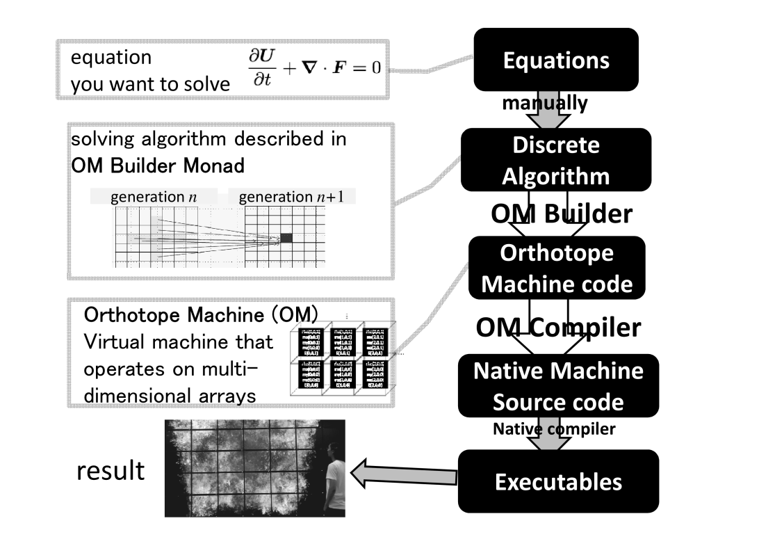
Figure 1: The Overall Picture.

2.1 Overall Design

Paraiso is to tackle the ambitious problem of generating fast and massively-parallel codes from human-friendly notations of algorithms. To divide the problem into major components, which may be conquered by different set of people, we set the overall design of Paraiso, as illustrated in Fig. 1.

The users of Paraiso must manually invent a discretized algorithm for the partial differential equations they want to solve. The solving algorithms are described in Paraiso using Builder Monads. Builder Monads generate programs for Orthotope Machine (OM), a virtual parallel machine designed to denote parallel computations on multi-dimensional arrays. Then the back end OM compiler generates the native machine source codes such as C++ and CUDA. Finally, native compilers translate them to executable codes.

When someone translates a simulation algorithm in his mind, to different languages such as Fortran, C and CUDA, he starts from building mathematical notations in his mind, and then gradually decomposes it to machine level. There should be the last common level that is independent of the detail of the target languages or the target hardwares. The level consist of very primitive operations on arrays. Orthotope Machine (OM) is designed to capture this level: The instruction set of the OM is kept as compact as possible, while maintaining all the parallelisms found in the solving algorithms. In forthcoming technical report we plan to provide the formal definition of the Orthotope Machine.

Name and Module	Description
data :~, data Vec, class Vector, class VectorRing in Data.Tensor.TypeLevel	Tensor algebra library that provides type level information for the tensor rank and dimension. c.f. §2.4.
type Builder in Language.Paraiso.OM.Builder	The Builder Monad for constructing the data flow graphs for OMs. c.f. §2.5.
data OM in Language.Paraiso.OM	The Orthotope Machine(OM), a virtual machine with basic instructions for stencil computations and reductions. c.f. §2.2.
type Graph in Language.Paraiso.OM.Graph	The data-flow graph for the OM. c.f. §2.2, Fig. 2, Fig. 3.
type Annotation in Language.Paraiso.Annotation	The collection of annotations that are added to each OM data-flow graph node. c.f. §2.6, §3.1.
data Plan in Language.Paraiso.Generator.Plan	The fixed detail of the code to be generated such as amount of memories and what to do in each subroutine. c.f. Fig. 5. To see how a plan is fixed c.f. Fig. 7.
data Program in Language.Paraiso.Generator.Claris	The subset of C++ and CUDA syntax tree which is sufficient in generating codes in scope of Paraiso. c.f. Fig. 5.
newtype Genome in Language.Paraiso.Tuning.Genetic	The set of annotations that belongs to an individual encoded as a string of letters, with which one can mutate, cross and triangulate. The evolution algorithm is in §3.2.

Table 1: List of concepts introduced by our work.

In order to generate the OM data-flow graphs from tensor expressions, and to translate them as native programs and further to apply manual and automated tuning over them, Paraiso introduces a number of abstract concepts centered around the OM. These components are quite orthogonal to each other, and some may even be useful outside the context of Paraiso. Table 1 summarizes those concepts, and provides pointers to the source code and the sections in this paper.

Orthotope Machine will endure the change in parallel languages and hardwares, as long as there are needs for explicit solvers of PDEs. Language/hardware designers can access to various applications for test and practical purpose, once they support translation from Orthotope Machine to their language. With Orthotope Machine as an interface, we can combine various stencil computation applications with state-of-the-art techniques developed so far, such as cache-friendly data structures [4], overlapping communication with computation [12, 5] or heterogeneous utilization of CPU/GPU [13]. On the other hand, various concepts of numerical simulations has been decomposed to elemental calculations before the OM level, so the problem of how to build a parallel computation from components such as new spatial interpolations, time marching methods and approximate Riemann solvers, can be addressed and developed separately from the detail of the hardware. To achieve such orthogonality is one of the aims of the Paraiso project.

2.2 Outline of The Orthotope Machine(OM)

The Orthotope Machine (OM) is a virtual machine much like vector computers. Each register of OM is multidimensional array of infinite size. Arithmetic operations of OM work in parallel on each mesh, or loads from neighbor cells. We have no intention of building a real hardware: OM is a thought object to capture parallel algorithms to data-flow graphs without losing parallelism.

The instruction set of OM resembles those of historical parallel machines such as PAX computer [14], and is subset of partitioned global address space (PGAS) languages such as XcalableMP [15].

Each instance of OM have a specific dimension (e.g. a two-dimensional OM of size $N0\times N1$). The variables of OM are either arrays of that dimension, or a scalar value. All of the arrays must have a common size. The actual numbers ($N0,N1$) are fixed at native code generation phase. We say that arrays are variable with Local Realm , while the scalars are variable with Global Realm.

OM has a set of Static variables which denotes the current state of the simulation. Each Static variable has a string name. OM has a set of Kernels — they are subroutines for updating the Static variables. Inside each Kernel, you can generate Temporal values in static single assignment (SSA) manner.

To summarize, the lifetime of an OM variable is either Static or Temporal, and the Realm of an OM variable is either Local or Global. Static variables survive multiple Kernel calls, while Temporal variables are limited to one Kernel. Local variables are arrays. Global variables are scalar values; in other words, they are arrays whose elements are globally the same.

OM cannot handle array of structures; Local variables may contain only simple objects such as Bool or Double, but not composite ones such as complex numbers or vectors. Nevertheless we can easily use such composite concepts in Paraiso programs at Builder Monad level and translate them to OM instructions, for example by using the applicative programming style [16].

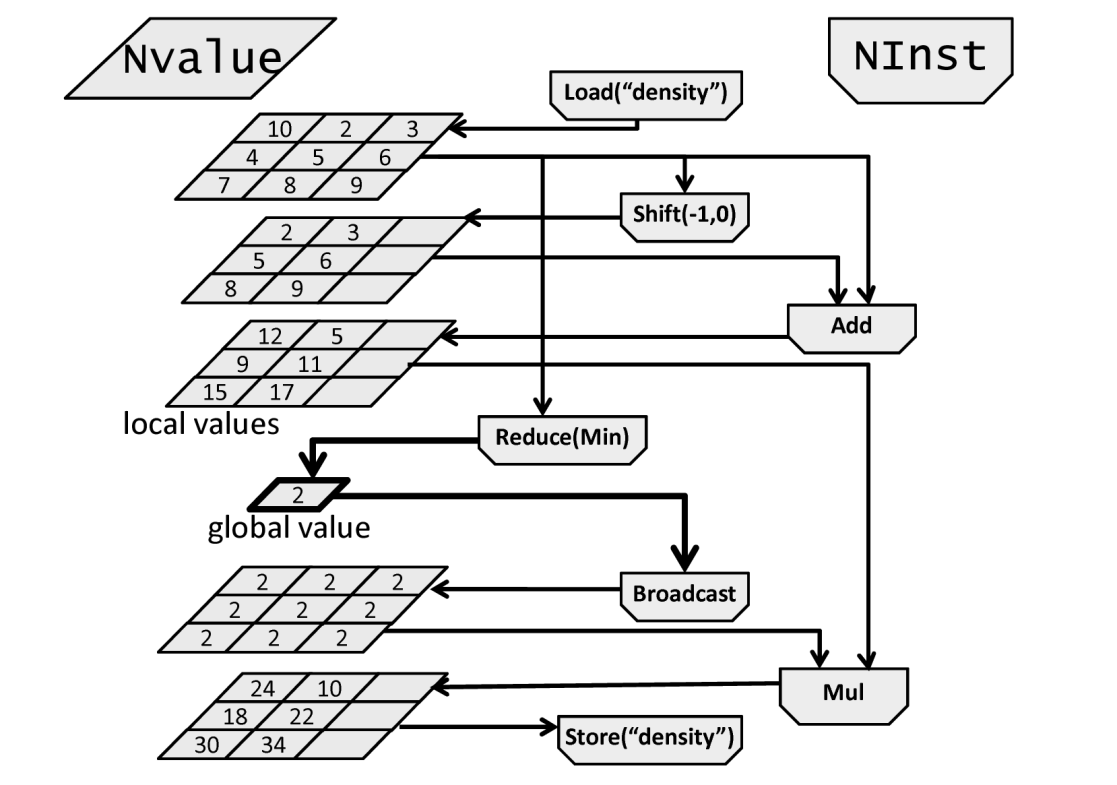
Figure 2: A data-flow graph for Orthotope Machine(OM).

An OM Kernel is a directed bipartite graph consisting of NInst nodes and NValue nodes, as illustrated in Fig. 2. Each node has arity :: a -> (Int, Int), number of incoming and outgoing edges. NValue nodes have arity of (1,$n$), where $n$ is the number of NInst nodes that uses the value and can be an arbitrary integer. Arities of NInst nodes are inherited from the instructions they carry.

OM has nine instructions:

data Inst vector gauge
  = Imm Dynamic
  | Load StaticIdx
  | Store StaticIdx
  | Reduce R.Operator
  | Broadcast
  | Shift (vector gauge)
  | LoadIndex (Axis vector)
  | LoadSize (Axis vector)
  | Arith A.Operator

Here, we limit ourselves to C pseudo-code of OM instruction semantics. The formal definition of the OM will be in forthcoming technical reports. Note that we do not translate the OM instructions one by one to C codes listed here. Instead, the instructions are merged into sub-graphs and then translated to C loops (or CUDA kernels) with much larger bodies, to make efficient use of computation resource and memory bandwidth (c.f. §3.1).

Imm

arity $(0,1)$: load constant value. Its output can be either Global or Local NValue node. For example, for a Local Temporal variable a,

a <- imm 4.2

means

for(int j=0; j<N1; ++j) {
  for(int i=0; i<N0; ++i) {
    a[j][i] = 4.2;
  }
}

Load

arity $(0,1)$: read from static variable to temporal variable. The realms of the static and temporal variable must match, and can be either of Global or Local. For example, for a Local Temporal variable a and Local Static variable density,

a <- load "density"

means

for(int j=0; j<N1; ++j) {
  for(int i=0; i<N0; ++i) {
    a[j][i] = density[j][i];
  }
}

Store

arity $(1,0)$: write a temporal variable to a static variable. The realms of the static and temporal variable must match, and can be either of Global or Local.

store "density" <- a

means

for(int j=0; j<N1; ++j) {
  for(int i=0; i<N0; ++i) {
    density[j][i] = a[j][i];
  }
}

Reduce

arity $(1,1)$: convert a local variable to a global one with a specified reduction operator.

b <- reduce Min <- a

means

b = a[0][0];
for(int j=0; j<N1; ++j) {
  for(int i=0; i<N0; ++i) {
    b = min(b,a[j][i]);
  }
}

Broadcast

arity $(1,1)$: convert a global variable to a local one.

b <- broadcast <- a

means

for(int j=0; j<N1; ++j) {
  for(int i=0; i<N0; ++i) {
    b[j][i] = a;
  }
}

Shift

arity $(1,1)$: takes a constant vector and an input local variable. Move each cell to its neighbor.

b <- shift (1,5)<- a

means

for(int j=0; j<N1-5; ++j) {
  for(int i=0; i<N0-1; ++i) {
    b[j+5][i+1] = a[j][i];
  }
}

LoadIndex

arity $(0,1)$: get coordinate of each cell. The output must be a Local value.

b0 <- loadIndex 0
b1 <- loadIndex 1

means

for(int j=0; j<N1; ++j) {
  for(int i=0; i<N0; ++i) {
    b0[j][i] = i;
  }
}
for(int j=0; j<N1; ++j) {
  for(int i=0; i<N0; ++i) {
    b1[j][i] = j;
  }
}

LoadSize

arity $(0,1)$: get array size. The output must be a Global value.

c0 <- loadSize 0
c1 <- loadSize 1

means

c0 = N0;
c1 = N1;

Arith

perform various arithmetic operations. The arity of this NInst node is inherited from its operator. The realms of the inputs and outputs must match, and can be either of Global or Local. If Local, array elements at matching index are operated in parallel (i.e. zipWith).

For example,

c <- arith Add a b <- a,b

means

for(int j=0; j<N1; ++j) {
  for(int i=0; i<N0; ++i) {
    c[j][i] = a[j][i] + b[j][i];
  }
}

2.3 An Example of Orthotope Machine Data-Flow Graph

Here we show the use case of the Orthotope Machine operators introduced in §2.2 within a simple PDE solver. We solve the following linear wave equation:

$$\frac{\partial^{2}f}{\partial t^{2}}-c^{2}\frac{\partial^{2}f}{\partial x^{2}}=0,$$ (1)

where $t$ is time, $x$ is one-dimensional space coordinate and $c$ is the signal speed.

By introducing the time derivative $g={\partial f}/{\partial t}$, Eq. (1) is rewritten as following system of first-order PDEs:

$$\frac{\partial f}{\partial t}=g,$$ (2)

$$\frac{\partial g}{\partial t}=c^{2}\frac{\partial^{2}f}{\partial x^{2}},$$ (3)

and satisfies the following conservation law:

$$\frac{d}{dt}E=0,$$ (4)

$$E\equiv\int\left(\frac{c^{2}}{2}\left(\frac{\partial f}{\partial x}\right)^{2}+\frac{g^{2}}{2}\right)dx.$$ (5)

We will write a Paraiso code that simulate the discrete system of Eqs. (2,3) and tests the conservation law.

Let $f^{n}[\mathrm{i}]$ denote the discrete field where $n$ and $\mathrm{i}$ are the discrete time and space coordinate, respectively. We choose the following 2nd-order, Lax-Wendorf and Leap Frog scheme to solve Eqs. (2,3) :

$$f^{n+1}[\mathrm{i}]=f^{n}[\mathrm{i}]+\Delta t\,g^{n}[\mathrm{i}],$$ (6)

$$g^{n+1}[\mathrm{i}]=g^{n}[\mathrm{i}]+\frac{c^{2}\,\Delta t}{\Delta x^{2}}\left(f^{n+1}[\mathrm{i}+1]+f^{n+1}[\mathrm{i}-1]-2f^{n+1}[\mathrm{i}]\right),$$ (7)

and measure the following discrete form of the conserved quantity:

$$E^{n+1}\equiv\sum_{i=0}^{N-1}\left[\left(c^{2}\frac{f^{n+1}[\mathrm{i}+1]-f^{n+1}[\mathrm{i}-1]}{2\,\Delta x}\right)^{2}+\left(\frac{g^{n+1}[\mathrm{i}]+g^{n}[\mathrm{i}]}{2}\right)^{2}\right]\Delta x$$ (8)

proceed :: Builder Vec1 Int Annotation () proceed = do c <- bind $ imm 3.43 n <- bind $ loadSize TLocal (0::Double) $ Axis 0 f0 <- bind $ load TLocal (0::Double) $ fieldF g0 <- bind $ load TLocal (0::Double) $ fieldG dx <- bind $ 2 * pi / n dt <- bind $ dx / c f1 <- bind $ f0 + dt * g0 fR <- bind $ shift (Vec:~ -1) f1 fL <- bind $ shift (Vec:~ 1) f1 g1 <- bind $ g0 + dt * c^2 / dx^2 * (fL + fR - 2 * f1) store fieldF f1 store fieldG g1 dfdx <- bind $ (fR - fL) / (2*dx) store energy $ reduce Reduce.Sum $ 0.5 * (c^2 * dfdx^2 + ((g0+g1)/2)^2) * dx

Table 2: A Paraiso source code for solving discrete Eq. (6,7).

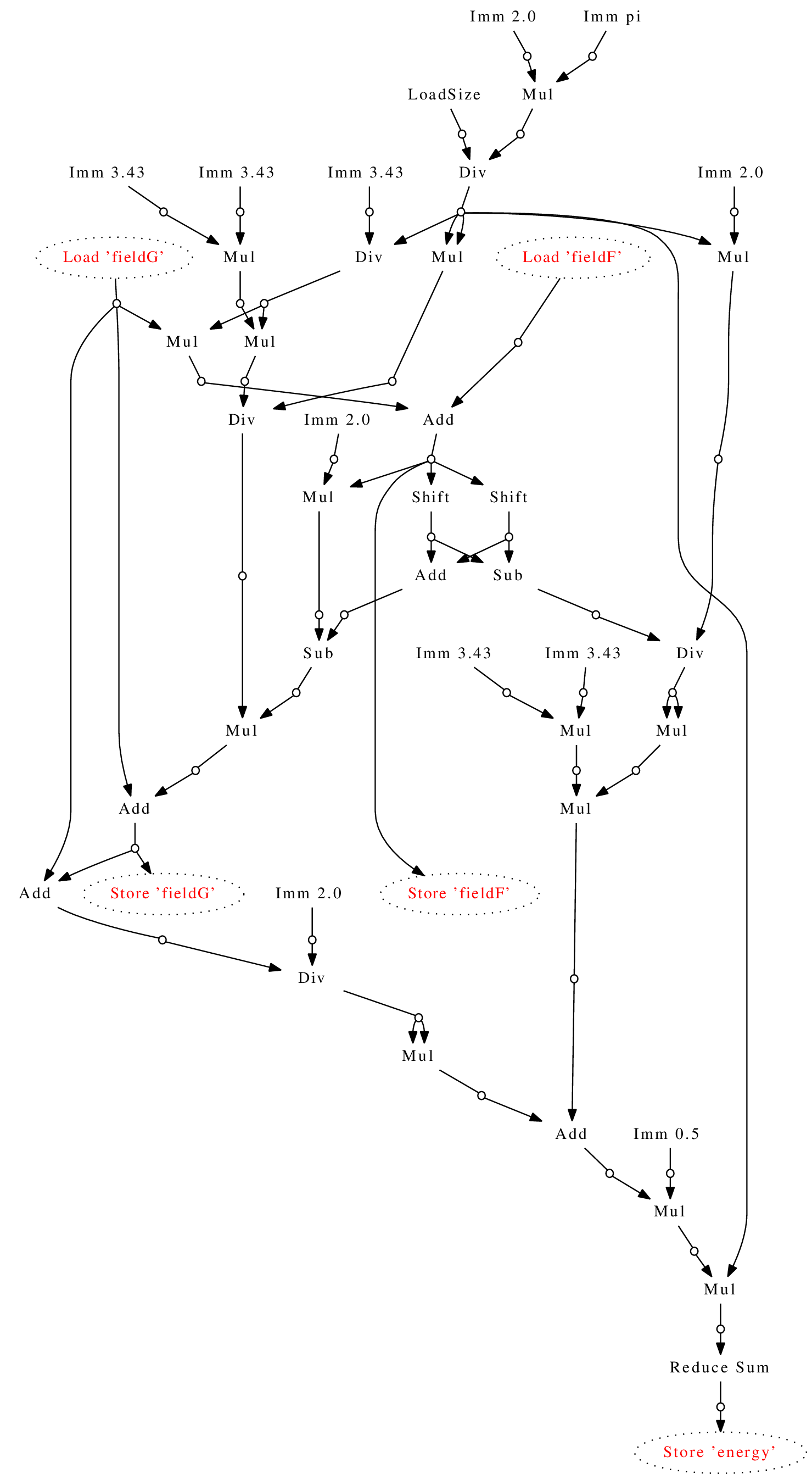
Figure 3: The Orthotope Machine data-flow graph generated from the Paraiso source code listed in Table 2. For brevity, NValue nodes are represented as little circles and only NInst nodes are shown; the Arith instruction nodes are replaced by arithmetic operators inside them, and the instruction arguments are not shown but for Load, Store and Reduce.

Table 2 shows the Paraiso implementation for the algorithm Eq. (6,7). The corresponding OM data-flow graph is visualized in Fig. 3. See how the data-flows from Load node to Store node. Here, we have $c=3.43$ and $0\leq x<2\pi$. We have performed numerical simulations using this program and the following initial condition:

$$f(x)=\sin(x),$$ (9)

$$g(x)=\cos(3x),$$ (10)

with resolution varying from $N=8$ to $N=3072$, and have confirmed that the fluctuation of discrete conserved quantity, Eq. (8) was smaller than of the order of $10^{-13}$.

2.4 Typelevel Tensor

We introduce typelevel-tensor library, to abstract over the dimensions; the use of tensor notations allow us to describe the algorithms for different dimensions in a single source code. The benefit of having information on tensor dimensions and ranks at the type-level is that we can detect erroneous operations like adding two tensors of different dimensions at compile time. Also we have much less need for explicitly mentioning the tensor dimensions in our programs, because the dimensions will be type-inferred.

Our approach is similar to that in [17], where two constructors Z and :. are used to inductively define multi-dimensional tuples. Their $n$-dimensional vectors are actually $n$-tuples, so it is possible that the set of $n$ elements consist of different types. In contrast, we needed that all the $n$ elements of a vector are of the same type, because we wanted to operate on them, for example by applying a same function to all of them.

So instead of [17]’s approach:

infixl 3 :.
data Z = Z
data tail :. head = tail :. head

We have these:

infixl 3 :~
data Vec a = Vec
data (n :: * -> *) :~ a = (n a) :~ a

Here, Vec is the type constructor for 0-dimensional vector, and :~ is a type-level function that takes the type constructor for $n$-dimensional vector as an argument and returns the type constructor for $n+1$-dimensional vector. We define type synonyms for successively higher vector:

type Vec0 = Vec
type Vec1 = (:~) Vec0
type Vec2 = (:~) Vec1
type Vec3 = (:~) Vec2

Vec0, Vec1, Vec2, and Vec3 are all types of kind * -> *, meaning that it takes one type (the element type) and returns another (the vector type). For example, the three-dimensional double precision vector type is Vec3 Double. Higher-rank tensors are defined as nested vectors; for example Vec3 (Vec3 Int) is a $3\times 3$ matrix of integers.

Since we know that all the elements of our tensor are of the same type a, we can make our tensors instances of Traversable type class [16, 18]:

instance Traversable Vec where
  traverse _ Vec = pure Vec
instance (Traversable n) => Traversable ((:~) n) where
  traverse f (x :~ y) = (:~) <$> traverse f x <*> f y

The benefit of making our tensors instances of Traversable is that we can traverse on them:

traverse :: Applicative f => (a -> f b) -> t a -> f (t b)

Here, suppose t is our tensor type-constructor and f is some context — for example, a code generation context. a and b are elements of our tensor. Then the type of the traverse function means that if we have code generators for the computation of one element (a -> f b), and we have a t a, a tensor whose elements are of type a, then we can deduce the code generator for computation of the entire tensor f (t b).

2.5 Builder Monad

Builder monad is a State monad whose state is the half-built data-flow graph of the Orthotope Machine. To represent the data-flow graph, we use Functional Graph Library (FGL) [19, 20]. Authors learned from the Q monad [21] how to encapsulate the construction process.

The graph carried by the State monad has the following type:

type Graph (vector :: *->*) (gauge :: *) (anot :: *)
  = FGL.Gr (Node vector gauge anot) Edge

data Node vector gauge anot =
  = NValue DynValue anot
  | NInst (Inst vector gauge) anot

data Edge
  = EUnord
  | EOrd Int

Graph takes three type arguments. vector :: *->* is a type constructor that denotes the dimension of the OM. gauge is the type for the indices of the arrays, which is usually an Int. anot is the type the nodes of the graph are annotated with. Such annotations are used to analyze and optimize the data-flow graph.

The three types vector, gauge, and anot are passed to the Nodes of the graph. Nodes are either NValue or NInst. Two types vector and gauge are further passed to the instruction type Inst, because instructions such as shift requires the information on the array dimension and indices. Every graph nodes are also annotated by type anot.

On the other hand, the edges contain none of the three types. They are just unordered edges EUnord or edges ordered by an integer EOrd Int. For example, we can exchange two edges going into addition instruction, but cannot exchange those into subtraction.

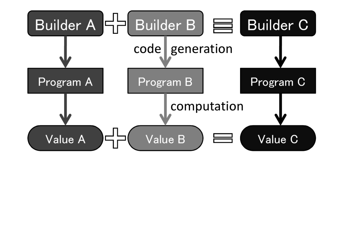
Figure 4: A commutative diagram of Builder Monad and computation.

We define various mathematical operations between Builder Monad in a consistent manner (c.f. Fig. 4). For any operator $\oplus$, Builder A $\oplus$ Builder B $=$ Builder C is defined by Value A $\oplus$ Value B $=$ Value C, where Value $i$ is the value computed by Program $i$ which is generated by Builder $i$. For example, a helper function that takes an operator symbol op, two builders builder1 and builder2, and create a binary operator for builder, is as follows:

mkOp2 :: (TRealm r, Typeable c) =>
         A.Operator                  -- ^The operator symbol
      -> (Builder v g a (Value r c)) -- ^Input 1
      -> (Builder v g a (Value r c)) -- ^Input 2
      -> (Builder v g a (Value r c)) -- ^Output
mkOp2 op builder1 builder2 = do
  v1 <- builder1
  v2 <- builder2
  let
      r1 = Val.realm v1
      c1 = Val.content v1
  n1 <- valueToNode v1
  n2 <- valueToNode v2
  n0 <-  addNodeE [n1, n2] $ NInst (Arith op)
  n01 <- addNodeE [n0] $ NValue (toDyn v1)
  return $ FromNode r1 c1 n01

We first extract the graph nodes from left hand side and right hand side builders in Builder context, add an NInst node that contains op symbol, add an NValue node after that, and return the node index.

In Haskell, defining mathematical operators between a data type is done by declaring the data type as an instance of the type class that manages the operator. In this sense type classes in Haskell are the parallels of algebraic structures such as group, ring and field, that manages addition, multiplication, and division, respectively. We use a Haskell package numeric-prelude that provides such algebraic structures [22].

For example, an Additive instance declaration of Builder is as follows:

instance (TRealm r, Typeable c, Additive.C c)
  => Additive.C (Builder v g a (Value r c)) where
  zero = return $ FromImm unitTRealm Additive.zero
  (+) = mkOp2 A.Add
  (-) = mkOp2 A.Sub
  negate = mkOp1 A.Neg

These type class instances, together with typelevel-tensor library, allows us to write tensor equations used in Paraiso application programs. Moreover, such equations are good for arbitrary instances of the type class. For example, here are the definition of momentum and momentum flux in our Euler equations solver:

momentum x = compose (\i -> density x * velocity x !i)
momentumFlux x =
  compose (\i -> compose (\j ->
    momentum x !i * velocity x !j + pressure x * delta i j))

These functions can be used to directly calculate momentum vector and momentum flux tensor whose components are of type Double. The very same functions are used to generate the solvers for CPUs and GPUs. At that time, their components are inferred to be Builder types. In addition to that, these functions can handle tensors of arbitrary dimensions.

2.6 Backend

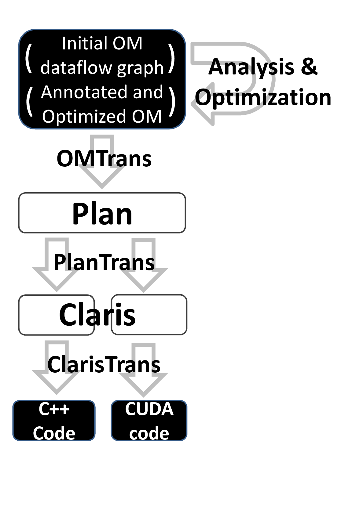
Figure 5: Backend.

The back end converts the data-flow graph of Kernels native codes, and create a C++ class corresponding to an OM. The code generation processes of Paraiso is illustrated in Fig. 5.

First, various analysis and optimizations are applied. Analysis and optimizations are functions that takes an OM and returns an OM, so we can combine them in arbitrary ways. Though some analysis are mandatory for code generation.

Paraiso has an omnibus interface for analysis and optimization using dynamic programming library Data.Dynamic in Haskell [23] :

type Annotation = [Dynamic]
add :: Typeable a => a -> Annotation -> Annotation
toList :: (Typeable a) => Annotation -> [a]
toMaybe :: (Typeable a) => Annotation -> Maybe a

Here, analyzers as well as human beings can add annotations of arbitrary type a to the graph. On the other hand, optimizers can read out annotations of what type they recognize and perform transformations on the data-flow graph. The set of annotations can be serialized to, and deserialized from genomes, which are binary strings used in automated tuning phase.

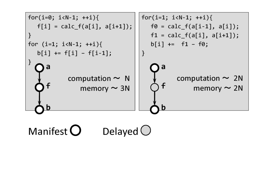
Figure 6: A Manifest - Delayed trade off. The left code requires less arithmetic units but consumes more memory and its bandwidth; The right code requires less memory and bandwidth in cost of more computations.

Examples of annotations are the choices of whether to store a value on memory and reuse or not to store and recompute it as is needed (c.f. Fig. 6); the boundary analysis result used for automatically adding ghost cells; dependency analysis; and labels used for dead code eliminations.

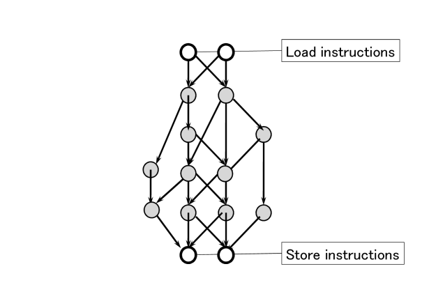
	(a) Some nodes need to be Manifest.
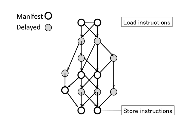
	(b) For each of other nodes, the genome specifies whether it is Manifest or Delayed.
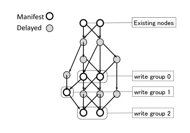
	(c) The sets of nodes that can be calculated in the same loop are greedily merged into write groups.
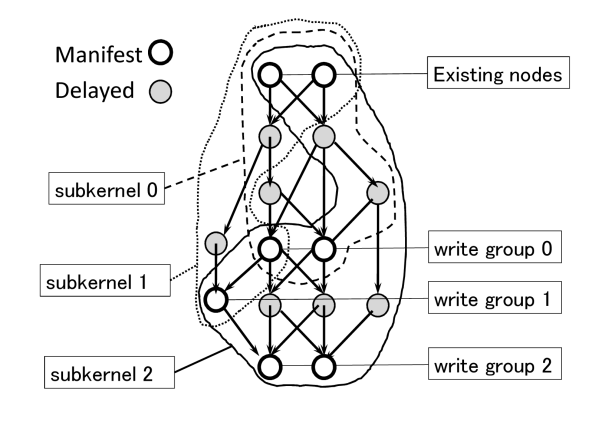
	(d) The Kernel is divided to multiple subKernels, each of which representing one write group. Each subKernel is in turn translated to a function in C or a __global__ function in CUDA.

Figure 7: How Paraiso generates a Plan from the given set of annotations.

Once the analysis and optimizations are done, an OM is translated to a code generation Plan. Here, decisions are made for how many memory are used, what portion of computation goes into a same subroutine, and so on. The nodes in data-flow graph are greedily merged as long as they have no dependence and can be calculated in the same loop (Fig. 7).

The Plan is further translated to CLARIS (C++-Like Abstract Representation of Intermediate Syntax). CLARIS is subset of C++ and CUDA syntax which is sufficient in generating codes in scope of Paraiso.

Finally, CLARIS is translated to native C++ or CUDA codes.

3 Automated Tuning Mechanism

3.1 Tuning Targets

The objects we want to optimize are the implementations of a partial differential equations solving algorithm. We call them individuals, adopting the genetic algorithm terminology. Each individual has a genome that encodes how it have chosen to implement the algorithm. The choices are (1) how much computation speed and memory bandwidth to use, (2) where to synchronize the computation, and (3) the CUDA kernel execution configuration. The fitness of the genome is the benchmark score of the generated code, measured in cups (the number of fluid cells updated per second) which we want to maximize.

A simple example program Fig. 6 indicates that we have implementation choices for intermediate variables: whether to store its entire contents on the memory (Manifest) or not to store them and recompute them as they’re needed (Delayed). The terms Manifest and Delayed are inherited from REPA [17]. If we increase the number of Manifest nodes, we consume less arithmetic units but more memory and its bandwidth; decreasing the number of Manifest nodes have the opposite effect. There are two extreme configurations, one is making as many nodes Manifest as possible and the other is making as few nodes Manifest as possible. In most cases both of them result in poor performance and moderate configurations are faster. Paraiso generate codes for many possible combinations of Manifest / Delayed choices (Fig. 7) and searches for such configurations by automated tuning.

Another tuning done by Paraiso is the choice of synchronization points. In CUDA, inserting __syncthreads(), especially before load/store instructions cause the next instruction to coalesce and increase the speed of the program. Inserting too much synchronization, on the other hand, is a waste of time. Again, Paraiso searches for better configurations by automated tuning.

The last tuning done by Paraiso is to find the optimal CUDA kernel execution configuration, i.e. how many CUDA threads and thread blocks to be launched simultaneously. These tuning items summed, the genome size is approximately $6000$ bits for our hydrodynamics solver, which means that there are $2^{6000}$ possible implementations. Brute-force searching for the fastest implementation from this space is inutile and in the first place impossible. Instead, the goal of Paraiso is to stochastically solve such a global optimization problem in this genome space, where the function to be optimized is the benchmark score of the PDE solver generated from the genome.

proceed = do x <- bind $ loadLD density y <- bind $ x * x z <- bind $ y + y store density z		proceed = do x <- bind $ Anot.add Sync.Pre <?> loadLD density y <- bind $ Anot.add Alloc.Manifest <?> x * x z <- bind $ y + y store density z
Their genome:
AAAAACAAAAAAACAAAAAA		AAAAACAAAAAAACAACGAA
The generated header file, abbreviated:
class Hello { public:device_vector<double> static_0_density; public:device_vector<double> manifest_0_5; public:void Hello_sub_0 (const device_vector <double> &a1, device_vector <double> &a5); public:void proceed (); };		class Hello { public:device_vector<double> static_0_density; public:device_vector<double> manifest_0_3; public:device_vector<double> manifest_0_5; public:void Hello_sub_0 (const device_vector<double> &a1, device_vector < double >&a3); public:void Hello_sub_1 (const device_vector<double> &a3, device_vector<double> &a5); public:void proceed (); };
The generated .cu program file, abbreviated:
__global__ void Hello_sub_0_inner (const double *a1, double *a5) { for (int i = INIT; (i) < (256); (i) += STRIDE) { int addr_origin = i; double a1_0 = (a1)[(addr_origin) + (0)]; double a3_0 = (a1_0) * (a1_0); ((a5)[addr_origin]) = ((a3_0) + (a3_0)); } } void Hello::proceed () { Hello_sub_0 (static_0_density, manifest_0_5); (static_0_density) = (manifest_0_5); }		__global__ void Hello_sub_0_inner (const double *a1, double *a3) { for (int i = INIT; (i) < (256); (i) += STRIDE) { int addr_origin = i; __syncthreads (); double a1_0 = (a1)[(addr_origin) + (0)]; ((a3)[addr_origin]) = ((a1_0) * (a1_0)); } } __global__ void Hello_sub_1_inner (const double *a3, double *a5) { for (int i = INIT; i < (256); (i) += STRIDE) { int addr_origin = i; double a3_0 = (a3)[(addr_origin) + (0)]; ((a5)[addr_origin]) = ((a3_0) + (a3_0)); } } void Hello::proceed () { Hello_sub_0 (static_0_density, manifest_0_3); Hello_sub_1 (manifest_0_3, manifest_0_5); (static_0_density) = (manifest_0_5); }

Table 3: An example of changes in the genome and the implemented algorithm caused by annotations.

Table 3 shows a simple Paraiso kernel and how its genome and implementation is altered by adding annotations. This kernel named proceed performs the following calculations:

$$\begin{array}[]{l}\mathrm{foreach}\ {\mathbf{i}}:\\ x=\mathrm{density}[{\mathbf{i}}]\\ y=x\times x\\ z=y+y\\ \mathrm{density}[{\mathbf{i}}]=z\end{array}$$ (16)

It first loads from an array named density, performs a multiplication, then an addition, and then stores the result to density again.

The header file on the right side of the Table 3, compared to the left one, allocates an additional device_vector and declares an additional subkernel as results of a Manifest annotation. The right .cu file, compared to the left one, differs in two points: one is that it performs the multiplication y = x * x and the addition z = y + y in separate CUDA kernels and stores the intermediate result to the additional device_vector, which is yet another result of the Manifest annotation. Another difference is that it calls __syncthreads() just before the load instruction, which is the result of the synchronization annotation.

3.2 Parallel Asynchronous Genetic Simulated Annealing

Simulated annealing has been widely used to solve global optimization problems. However, a standard simulated annealing method is not suitable for parallelization, and if the annealing schedule (how we cool down the temperature as function of time) is too quick, it tends to fall into local minima. Replica-exchange Monte Carlo method [24] solves these drawbacks by introducing multiple replicas of heat baths with different temperatures, and by allowing replica exchange between adjacent heat baths. Thus, replicas can be computed in parallel, and the annealing schedule is spontaneously managed by replica migration.

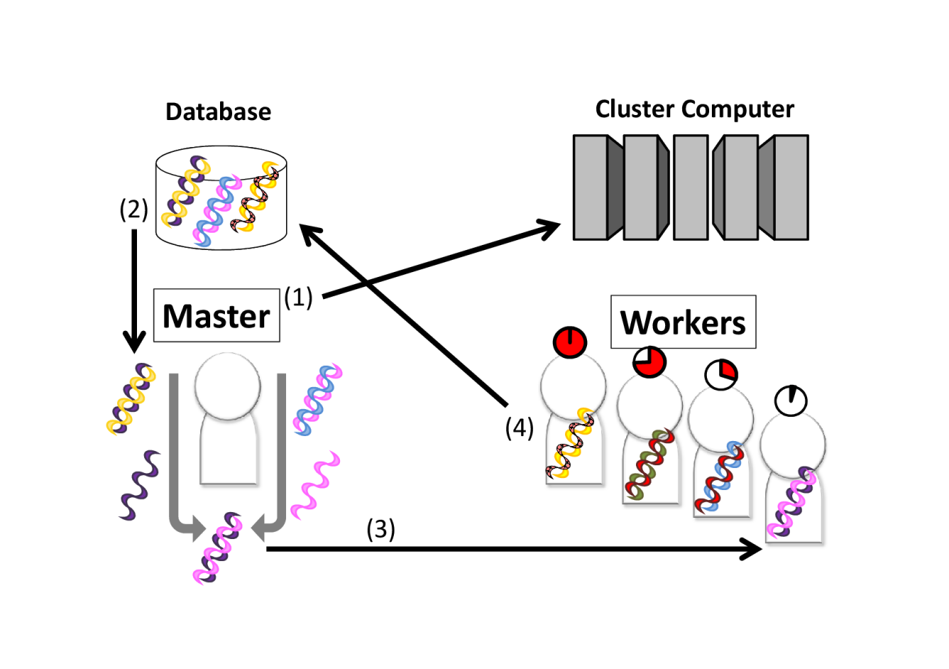
Figure 8: The master/worker model of parallel asynchronous genetic simulated annealing used for automated tuning in Paraiso. (1) The master periodically monitors for vacancy in the cluster computer system. (2) When a vacancy is found, the master creates a new individual from several genomes obtained from the database by performing draws of temperature $T$. (3) The master creates a worker job that generates native program from the genome and measures its speed. (4) Each worker writes the benchmark result to the database and quit as soon as it finishes its assigned measurements.

We further extend this method to fit into benchmark based tuning on shared cluster computer systems. First, in shared systems it is hard to maintain a fixed number of replicas because the available amount of nodes changes with time. Second, it is not efficient to perform replica-exchange synchronously, since the wall clock time required to calculate the fitness function varies with replicas. For these two reasons, we modify replica-exchange Monte Carlo method to a master/worker model (c.f. Fig. 8), where a master asynchronously launches varying number of workers in parallel.

The master holds the genomes and scores of all the past individuals in a database (DB). The role of the master is to draw individuals from the DB, to create new individuals using their genomes, and to launch the workers when the computer resource is available. The role of the workers, on the other hand, is to generate codes from the given genome, to take the benchmark, and to write the results into the DB.

In this way we can launch any number of workers asynchronously as long as the DB is not a bottleneck. In addition to that, we eliminate a common weak point of simulated annealing and genetic algorithms — that individuals of older generation are overwritten and are inaccessible.

For each individual $I$, the generated code is benchmarked 30 times. We record the mean $\mu(I)$ and the sample standard deviation $\sigma(I)$ of the score. It is important to record the deviation. When we benchmark each individual only once, some individuals receive over-evaluated score by chance, infest the system and tend to stall the evolution.

At the end of each benchmark, the individual is briefly tested if the state of the simulation has developed substantially from the initial condition and there is no NaN (not a number). The test is chosen because not evolving at all and generating NaN are two dominant modes of failure, and the individual test time needs to be kept smaller than benchmark itself. If an individual fails a test, its score is $0$. At the end of a tuning experiment, the champion individual is extensively tested if it can reproduce various analytic solutions, which takes hours.

A draw is the operation to randomly choose an individual from the DB. Each draw has a temperature $T$. In a draw of temperature $T$, the probability the individual $I$ is chosen is proportional to

$$\exp\left(\frac{\mu(I_{\top})-\mu(I)+\sigma(I_{\top})+\sigma(I)}{T+\sigma(I_{\top})+\sigma(I)}\right),$$ (17)

where $I_{\top}$ is the individual with the largest $\mu(I)$.

Low-temperature draws strictly prefer high-score individuals while high-temperature draws does not care the score too much. And the difference small compared to $\sigma(I_{\top})+\sigma(I)$ is gracefully ignored.

Every time master creates a new individual, it chooses the draw temperature $T$ randomly, so that the probability density of $\log{T}$ is uniformly distributed between $\log(\sigma(I_{\top}))$ and $\log(\mu(I_{\top}))$.

To summarize, our method is a master/worker variant of replica-exchange Monte Carlo method [24], using genetic algorithms as neighbor generators. Thus, our method

• can utilize parallel and dynamically varying computer resource.

• can find global maximum without hand-adjusted annealing schedule.

• can combine independently-found improvements.

An extensive review on the applications of the evolutionary computation in astronomy and astrophysics is found in [25].

3.3 Three Methods of Birth for Generating New Individuals

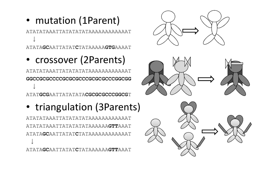
Figure 9: Three ways of generating new individuals.

We use three different methods of birth to generate new individuals (c.f. Fig. 9). The first method is mutation. We draw one individual from the database (DB), take its genome, overwrite it randomly and create a new genome. The second method is crossover. We draw two individuals from the DB, split their genomes at several random points and exchange the segments. The third method is triangulation, or three-parent crossover.

Multi-parent crossovers are crossovers that takes more than two parents and create one or multiple children. The proposed multi-parent crossover methods include taking bit-wise majority vote [26, 27] and exchanging segments between multiple parents [28]. Multi-parent crossovers for real-number coded genomes are also studied [29]. The novelty of our three-parent crossover (triangulation) is to take the scores of the parents into consideration. Triangulation is designed to efficiently combine independent improvement found in sub-problems.

FFTW [1] uses the divide and conquer approach to its target problems. It first recursively decomposes large FFT problem into smaller ones and solves the optimization problem from smaller part. In contrast, Paraiso deals with monolithic data-flow graphs. It is not obvious how to decompose them into subgraphs — decompositions are actually the target of optimization. Therefore, we optimize subgraphs in vivo; we optimize subgraphs keeping them embedded into the entire graph.

Base	0	0	0	0	1	1	1	1
Secondary	0	0	1	1	0	0	1	1
Primary	0	1	0	1	0	1	0	1
Child	0	1	1	1	0	0	0	1

Table 4: Binary operation table for triangulation.

Aiming to merge two distinct optimized subgraphs, we draw three individuals from the DB. Then we sort them in ascending order of the score and name them Base, Secondary and Primary. We perform bit-wise operation as in Table 4 to create their child. For each bit, if at least one of Primary or Secondary has been changed from Base, then we adopt the change.

When creating a new individual, the master chooses mutation, crossover, or triangulation at equal probability of $1/3$. Then the master draws the needed number of parents from the DB. If two of the parents are the same the master retries the draws. Otherwise, the master creates a child with the chosen method of birth. Then if the genome of the newly created individual is already in the DB, the master discards the individual and retries the mutation until it gets a genome not found in the DB. With each retry, draw temperature $T$ is multiplied by $1.2$, so that the master eventually succeed in creating a new genome.

4 Tuning Experiments

4.1 The Target Program

We implemented a 2nd order compressible hydrodynamics solver [30] in Paraiso, and then optimize it. Here we detail numerical scheme.

Let $A_{a},B_{ab},...$ denote tensor indices for tensor $A,B,...$. Let $[{\mathbf{i}}],[{\mathbf{j}}],...$ denote array indices which is a $d$-tuple of integer where $d$ is the dimension. Values integrated over cell volumes are given integer indices, and values integrated over cell surfaces are given indices with one half-integer and $d-1$ integers. For example, $A_{y}[{\mathbf{i}}]$ is the volume integral of $y$-component of a vector $A$ over the cell ${\mathbf{i}}$, and $B_{xz}[{\mathbf{i}}+\frac{1}{2}{\mathbf{e}}_{x}]$ is the surface integral of $xz$-component of a rank-2 tensor $B$ over the $+x$ surface of cell ${\mathbf{i}}$.

The equations of compressible hydrodynamics have $d+2$ degrees of freedom. The primitive variables $\mathbf{V}$ and the conserved variables $\mathbf{U}$ are the two representations of the degrees of freedom. The flux variables $\mathbf{F}$ are calculated from $\mathbf{U}$ or $\mathbf{V}$, as follows :

$${\mathbf{V}}=\left(\begin{array}[]{c}\rho\\ v_{a}\\ p\end{array}\right),$$ (21)

$${\mathbf{U}}=\left(\begin{array}[]{c}\rho\\ m_{a}\\ E\end{array}\right),$$ (25)

$${\mathbf{F}}_{a}=\left(\begin{array}[]{c}u_{a}\\ u_{a}m_{b}+p\delta_{ab}\\ u_{a}E+u_{a}p\end{array}\right).$$ (29)

where $\rho$ , $v_{a}$, $m_{a}$, $p$ and $E$ are the density, the velocity, the momentum, the pressure and the total energy, respectively, The primitive and conserved variables are related by $m_{a}=\rho v_{a}$, $E=E_{i}(p)+\frac{1}{2}\rho v^{2}$ where $E_{i}$ is the internal energy of the gas. By assuming the adiabatic equation of state for perfect gas, $E_{i}(p)=(\gamma-1)^{-1}p$ where $\gamma$ is the ratio of specific heats.

We numerically solve the Euler equations $\partial_{t}{\mathbf{U}}=\partial_{a}{\mathbf{F}}_{a}$ , or more specifically:

$$\partial_{t}\rho = \partial_{a}(\rho v_{a}),$$ (30)

$$\partial_{t}m_{b} = \partial_{a}(u_{a}m_{b}+p\delta_{ab}),$$ (31)

$$\partial_{t}E = \partial_{a}(u_{a}E+u_{a}p).$$ (32)

The numerical method we used is as follows, based on a function $\mathrm{Flux}_{a}(\mathbf{U0})$ which calculates the fluxes across the cell surfaces using a Riemann solver. $\mathrm{Flux}_{a}(\mathbf{U0})$ is defined as follows. First, $\mathbf{V0}$ are the primitive variables calculated from $\mathbf{U0}$:

$$\mathbf{V0}={\mathbf{V}}(\mathbf{U0}).$$ (33)

The interpolated primitive variables $\mathbf{VL}$ and $\mathbf{VR}$ are

$$(\mathbf{VR}[{\mathbf{i}}-{\textstyle\frac{1}{2}}{\mathbf{e}}_{a}],\mathbf{VL}[{\mathbf{i}}+{\textstyle\frac{1}{2}}{\mathbf{e}}_{a}])=$$

$$\hskip 28.45274pt\mathrm{Interpolate}(\mathbf{V0}[{\mathbf{i}}-{\mathbf{e}}_{a}],\mathbf{V0}[{\mathbf{i}}],\mathbf{V0}[{\mathbf{i}}+{\mathbf{e}}_{a}]),$$ (34)

where we use piecewise linear interpolation with minbee flux limiter [31, 30]:

$$\begin{array}[]{lrcl}\lx@intercol\mathrm{Interpolate}(\mathit{y0},\mathit{y1},\mathit{y2})=(\mathit{y1}-{\textstyle\frac{1}{2}}\mathit{dy},\mathit{y1}+{\textstyle\frac{1}{2}}\mathit{dy})\ \ \mathrm{where}\hfil\lx@intercol\\ &\mathit{dy01}&=&\mathit{y1}-\mathit{y0}\\ &\mathit{dy12}&=&\mathit{y2}-\mathit{y1}\\ &\mathit{dy}&=&\left\{\begin{array}[]{lll}0&\mathrm{if}&\mathit{dy01}\cdot\mathit{dy12}<0\\ \mathit{dy01}&\mathrm{if}&|\mathit{dy01}|<|\mathit{dy12}|\\ \mathit{dy12}&\lx@intercol\mathrm{otherwise}\hfil\lx@intercol.\end{array}\right.\\ \end{array}$$ (42)

Then, fluxes across the boundaries are defined using the HLLC Riemann solver [32].

$${\mathbf{F}}_{a}[{\mathbf{i}}+{\textstyle\frac{1}{2}}{\mathbf{e}}_{a}] = \mathrm{HLLC}_{a}(\mathbf{VL}[{\mathbf{i}}+{\textstyle\frac{1}{2}}{\mathbf{e}}_{a}],\mathbf{VR}[{\mathbf{i}}+{\textstyle\frac{1}{2}}{\mathbf{e}}_{a}]).$$ (43)

This is the flux defined by $\mathrm{Flux}_{a}(\mathbf{U0})$. Then, linear addition of flux to conserved variable $\mathrm{AddFlux}(\Delta t,\mathbf{F}_{a},\mathbf{U})$ is defined by

$$\mathbf{U2}=\mathrm{AddFlux}(\Delta t,\mathbf{F}_{a},\mathbf{U1})$$ (44)

$$\Leftrightarrow \mathbf{U2}[{\mathbf{i}}]=\mathbf{U1}[{\mathbf{i}}]+\sum_{a}\frac{\Delta t}{\Delta r_{a}}\left(\mathbf{F}_{a}[{\mathbf{i}}-{\textstyle\frac{1}{2}}{\mathbf{e}}_{a}]-\mathbf{F}_{a}[{\mathbf{i}}+{\textstyle\frac{1}{2}}{\mathbf{e}}_{a}]\right),$$

where $\Delta r_{a}$ is the mesh-size along the $a$-axis. Using these notations, we construct the second-order time marching as follows, where $\Delta t$ is the time step determined by the CFL-condition:

$$\mathbf{F0}_{a} = \mathrm{Flux}_{a}(\mathbf{U0})$$ (45)

$$\mathbf{U1} = \mathrm{AddFlux}({\textstyle\frac{1}{2}}\Delta t,\mathbf{F0}_{a},\mathbf{U0})$$ (46)

$$\mathbf{F1}_{a} = \mathrm{Flux}_{a}(\mathbf{U1})$$ (47)

$$\mathbf{U2} = \mathrm{AddFlux}(\Delta t,\mathbf{F1}_{a},\mathbf{U0})$$ (48)

$\mathbf{U2}$ is the set of conserved variables for the next generation.

Notice how we rely on human mind flexibility when we convey the algorithms in the forms like above. In languages like Fortran or C, we are often forced to decompose those expression into elemental expressions and the source codes tend to become longer. In Haskell, we can express these ideas in well-defined machine readable forms while keeping the compactness and flexibility as in above.

We declare both the primitive variables Eq. (21) and conserved variables Eq. (25) as instances of the type class Hydrable, the set of variables large enough for calculating any other hydrodynamic variables. We used the general form by default, and bind either the primitive or conserved variables when we need the specific form. By doing so requisite minimum number of conversion code between primitive and conserved variables are generated.

When we defined the minbee interpolation for a triplet of real numbers Eq. (42) and then applied it to primitive variables Eq. (34), we implicitly extended a function on real numbers to function on set of real numbers. In Haskell, we can define how any such generalized function application over the set of hydrodynamic variables should behave, just by making it an instance of Applicative type class.

When we calculate the space-derivatives of the fluxes in Eq. (44), the component of the flux we access (index $a$ in $\mathbf{F}_{a}$) and the direction in which we differentiate (indices $a$ in $[{\mathbf{i}}-{\textstyle\frac{1}{2}}{\mathbf{e}}_{a}]$ and $[{\mathbf{i}}+{\textstyle\frac{1}{2}}{\mathbf{e}}_{a}]$) should match. Although the flux $\mathbf{F}$ and the spatial array indices ${\mathbf{i}}$ have very different types, Haskell’s type inference guarantees that they are both tensors of the same dimensions, and we can access both of them by the common tensor index $a$. And we can sum over $a$, because tensors are Foldable and their components are Additive. Tensors are Traversable as mentioned before, and any type constructors that are Traversable are also Foldable.

4.2 Annotating By Hand

ID	config	(1)	(2)	lines	subKernel	memory
Izanagi	$32\times 32$	D	D	13128	7	$52\times N$
Izanami	$448\times 256$	D	D	13128	7	$52\times N$
Iwatsuchibiko	$448\times 256$	M	D	17494	12	$68\times N$
Shinatsuhiko	$448\times 256$	D	M	3010	11	$68\times N$
Hayaakitsuhime	$448\times 256$	M	M	3462	15	$84\times N$

ID	score (SP)	score (DP)
Izanagi	$1.551\pm 0.0005$	$1.138\pm 0.000$
Izanami	$5.838\pm 0.004$	$3.091\pm 0.002$
Iwatsuchibiko	$5.015\pm 0.002$	$2.491\pm 0.001$
Shinatsuhiko	$42.682\pm 0.083$	$19.831\pm 0.021$
Hayaakitsuhime	$34.100\pm 0.110$	$15.632\pm 0.024$

Table 5: The codes annotated by hand and their performances. First four columns are the ID of the individuals, the CUDA kernel execution configuration, and the two choices of annotation — whether to Manifest or Delay (1) the result of spatial interpolation (2) the result of the Riemann solver. Next three columns are the properties of the generated codes as results of these choices made. They are namely the size of the code (number of lines), the number of subKernels in the code, the memory consumption in proportion to fluid cell number $N$. The last two columns are the speed of the generated codes for single precision (SP) and double precision (DP). The speed of the codes are measured by Mcups ($10^{6}$ cell update per second).

The interpolation code for Izanami:

interpolateSingle order x0 x1 x2 x3 | order == 1 = do return (x1, x2) | order == 2 = do d01 <- bind $ x1-x0 d12 <- bind $ x2-x1 d23 <- bind $ x3-x2 let absmaller a b = select ((a*b) ‘le‘ 0) 0 $ select (abs a ‘lt‘ abs b) a b d1 <- bind $ absmaller d01 d12 d2 <- bind $ absmaller d12 d23 l <- bind $ x1 + d1/2 r <- bind $ x2 - d2/2 return (l,r)

For Iwatsuchibiko, the last line is modified as follows:

return (Anot.add Alloc.Manifest <?> l, Anot.add Alloc.Manifest <?> r)

Table 6: An annotation made in Paraiso source code that causes the results of the interpolations to be stored on memory and reused.

Before we start the automated tuning experiment, we generate several individuals by hand. The initial individual Izanagi is the one with the least number of Manifest nodes as possible. Izanami is the same individual with the CUDA execution configuration suggested by the CUDA occupancy calculator. Based on it, we add several Manifest annotation and create new individuals (c.f. Table 5). Manual annotations are not blind-search process; each annotation has clear motivation such as “let us store the result of the Riemann solvers because it is computationally heavy”, “let us store the result of interpolations because it moves a lot of data,” etc. For example, the sample code in Table 6 shows the implementation of the piecewise linear interpolation with the minbee flux limiter, Eq. (42) in Paraiso, and how to annotate the return values of the limiter as Manifest.

We use Izanami as the base line of the benchmark, and use Izanagi as the initial individual of some experiment to see if the automated tuning can find out the optimal CUDA execution configuration by itself.

The codes are benchmarked on TSUBAME 2.0 cluster at Tokyo Institute of Technology. Each individual was benchmarked on a TSUBAME node with two Intel Xeon X5670 CPU(2.93GHz, 6 Cores $\times$ HT = 12 processors) and three M2050 GPU(1.15GHz 14MP x 32Cores/MP=448Cores).

The abstraction power of Builder Monad lets us change the code drastically with little modification. For example, Paraiso source code of Shinatsuhiko and Izanami differs by just one line of annotation. This introduces the 16 bits of difference in their genome, causing Shinatsuhiko generate a code that has $1/3$ lines, which contains four more subroutines, consume $1.31$ times more memory and is $6.42$ times faster.

4.3 Automated Tuning

RunID	prec.	initial score	wct	best ID/total	high score
GA-1	DP	$1.138\pm 0.000$	3870	20756 / 20885	$14.158\pm 0.002$
GA-S1	DP	$1.138\pm 0.000$	4120	33958 / 34328	$16.247\pm 0.002$
GA-DE	DP	$19.253\pm 0.044$	7928	41250 / 41386	$31.015\pm 0.032$
GA-D	DP	$19.253\pm 0.044$	8770	59841 / 68138	$34.968\pm 0.043$
GA-4	DP	$19.253\pm 0.044$	5811	39991 / 40262	$35.303\pm 0.035$
GA-F	SP	$42.682\pm 0.083$	2740	23019 / 23062	$53.300\pm 0.078$
GA-F2	SP	$42.682\pm 0.083$	4811	22242 / 24887	$53.656\pm 0.078$
GA-3D	SP	$24.638\pm 0.001$	5702	38146 / 39200	$45.443\pm 0.116$

Table 7: The statistics of auto-tuning experiments. The columns are RunID, precision, the score of initial individual, the wall-clock time for the experiment (in minutes), the ID of the best individual and the number of individuals generated, the high score (in Mcups). Experiments GA-1 and GA-S1 started with Izanagi, others started with Shinatsuhiko. GA-3D started with Shinatsuhiko, and solved 3D problems.

	mutation	crossover	triangulation
GB-333	$1/3$	$1/3$	$1/3$
GB-370	$1/3$	$2/3$	$0$
GB-307	$1/3$	$0$	$2/3$

Table 8: The probability of the master node attempting each method of birth in experiment series GB-*.

RunID	prec.	initial score	best ID/total	high score
GB-333-0	DP	$19.253\pm 0.044$	35294 / 40014	$25.343\pm 0.028$
GB-333-1	DP	$19.253\pm 0.044$	40256 / 40031	$26.402\pm 0.023$
GB-333-2	DP	$19.253\pm 0.044$	39206 / 40033	$32.758\pm 0.006$
GB-370-0	DP	$19.253\pm 0.044$	36942 / 39994	$24.698\pm 0.045$
GB-370-1	DP	$19.253\pm 0.044$	37468 / 40045	$28.339\pm 0.042$
GB-370-2	DP	$19.253\pm 0.044$	39719 / 40032	$31.669\pm 0.039$
GB-307-0	DP	$19.253\pm 0.044$	30320 / 40018	$21.744\pm 0.035$
GB-307-1	DP	$19.253\pm 0.044$	39358 / 40002	$26.349\pm 0.026$
GB-307-2	DP	$19.253\pm 0.044$	38107 / 40053	$27.412\pm 0.005$

Table 9: The statistics of GB-* experiment series. The columns are RunID, precision, the score of initial individual, the ID of the best individual and the number of individuals generated, the high score (in Mcups). Experiments started with Shinatsuhiko. The nine experiments were performed in parallel, and took 92252 minutes of wall-clock time.

Next, we performed several automated tuning experiments c.f. Table 7.

To distinguish the contribution of the three methods to generate new individuals, we also performed automated tuning experiments with either crossover or triangulation turned off. Table 8 shows the initial possibility of the master node attempting each method of birth. Note that the actual frequencies of crossover and triangulation are smaller than these value because the master may default to mutation. Table 9 shows the result of experiments. The resolutions were $1024^{2}$ for GA-1 and GA-S1, problems, $100^{3}$ for GA-3D problems and $512^{2}$ for other GA-* series. The resolutions were $512^{2}$ in GB-* series.

The automated tuning system can generate and benchmark approximately $10^{\prime}000$ individuals per day. $20-100$ workers were running at the same time. It takes a few days to tune up Izanami to speed comparable to Shinatsuhiko, or speed up Shinatsuhiko by another factor of $2$. The best speed obtained was $35.3$Mcups for double precision, and $53.7$Mcups for single precision. Our automated tuning experiments on 3D solvers mark $42.4$Mcups SP. These are competitive performances to hand-tuned codes for single GPUs; e.g. Schive et. al. [33] reports $30$Mcups per C2050 card (single precision, note that their code is 3D. Asuncióna et.al. [34] reports $6.8$Mcups per GTX580 card (single precision, 2D).

(a)	(b)	(c)

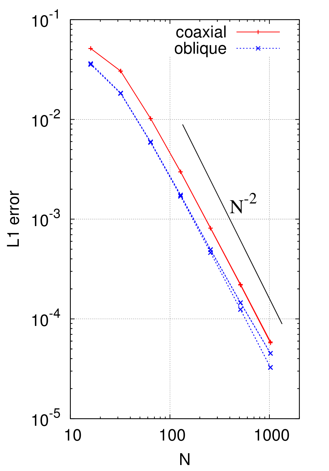
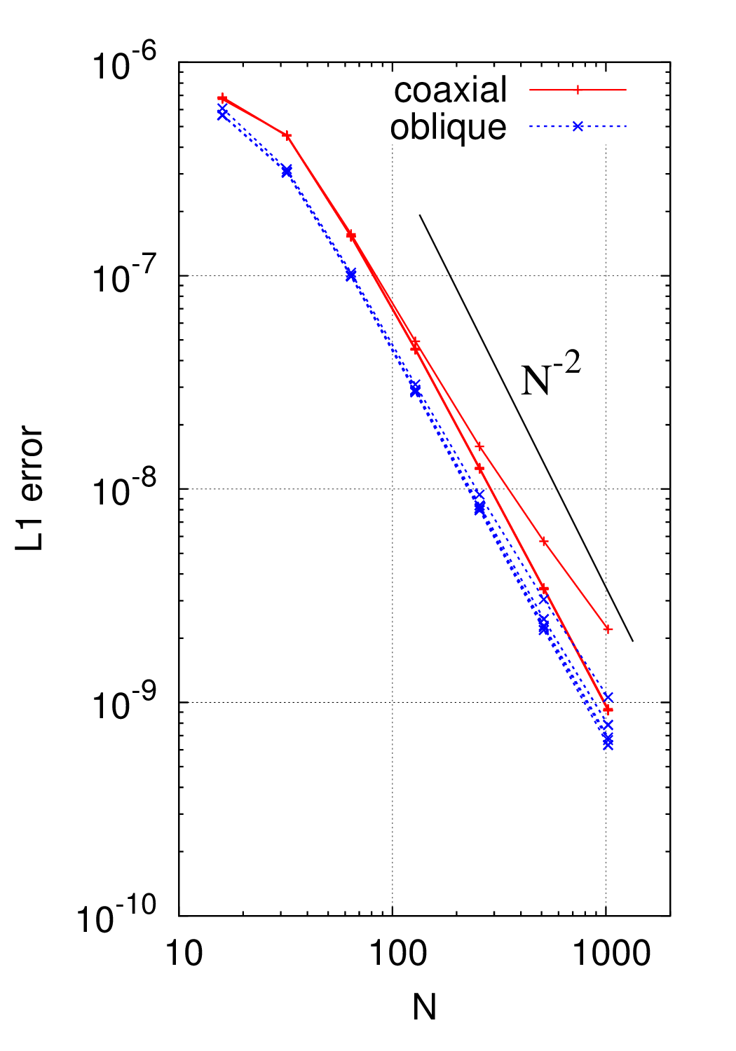
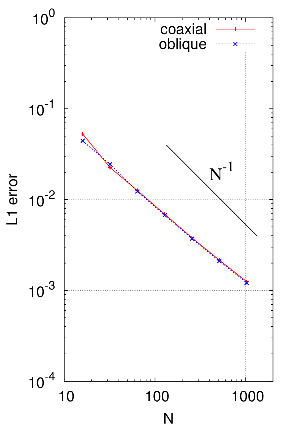
Figure 10: Convergence tests of the norm of the $L_{1}$ error vector of density field for (a)entropy waves, (b)sound waves and (c)shock-tube problem.

Fig. 10 shows the result of convergence tests for individuals GA-1.20756, GA-4.33991, GA-D.59841, GA-DE.41250, GA-S1.33958, Izanami and Shinatsuhiko. The resolution $N$ is varied from $16^{2}$ to $1024^{2}$. The codes are tested for entropy wave propagation, sound wave propagation and Sod’s shock-tube problem. The detail of test initial conditions are as follows. For all tests, numerically solved domains are $(0<x<1,0<y<1)$, out of which the analytic solutions are continuously substituted as boundary conditions. The system was numerically developed until $t=1$ for entropy wave and sound wave problems, and $t=0.125$ for shock tube problem, and then the numerical solutions were compared to analytic solutions using the norm of $L_{1}$ error vector.

The initial conditions are, for entropy wave problem:

$$\left\{\begin{array}[]{rcl}\rho(x,y)&=&2+\sin(2\pi x),\\ v_{x}(x,y)&=&1,\\ v_{y}(x,y)&=&0,\\ p(x,y)&=&1,\end{array}\right.$$ (53)

for sound wave problem:

$$\left\{\begin{array}[]{rcl}\rho(x,y)&=&\gamma\left(1+A\sin(2\pi x)\right)\\ v_{x}(x,y)&=&A\sin(2\pi x),\\ v_{y}(x,y)&=&0,\\ p(x,y)&=&1+\gamma A\sin(2\pi x),\end{array}\right.$$ (58)

where the amplitude $A=10^{-5}$, and for Sod’s shock-tube problem:

$$x<0.5\left\{\begin{array}[]{rcl}\rho(x,y)&=&1,\\ v_{x}(x,y)&=&0,\\ v_{y}(x,y)&=&0,\\ p(x,y)&=&1,\\ \end{array}\right.$$ (63)

$$x>0.5\left\{\begin{array}[]{rcl}\rho(x,y)&=&0.125,\\ v_{x}(x,y)&=&0,\\ v_{y}(x,y)&=&0,\\ p(x,y)&=&0.1.\\ \end{array}\right.$$ (68)

While the “coaxial” tests used the above initial conditions as they are, the “oblique” tests used the initial conditions rotated about $(x,y)=(0.5,0.5)$ for $60^{\circ}$.

5 Analysis on the Automated Tuning Experiments

5.1 Overview of The Simulated Evolution and Analyses

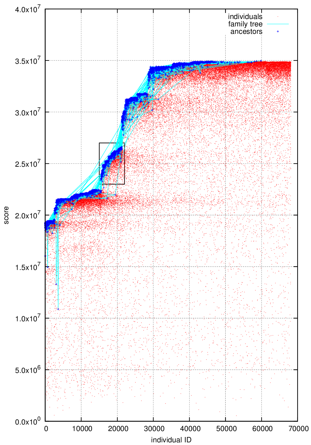
Figure 11: The ID and the scores (in cups) of all the individuals generated in automated tuning experiment GA-D. The individual with the highest score as well as its ancestors are marked by crosses, and each of them is connected to its parents with lines.

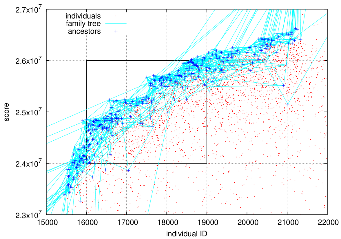
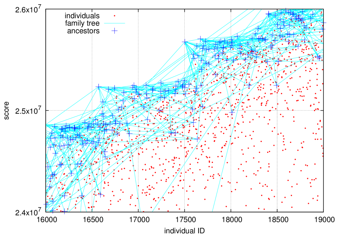
Figure 12: Two enlarged views of Fig. 11

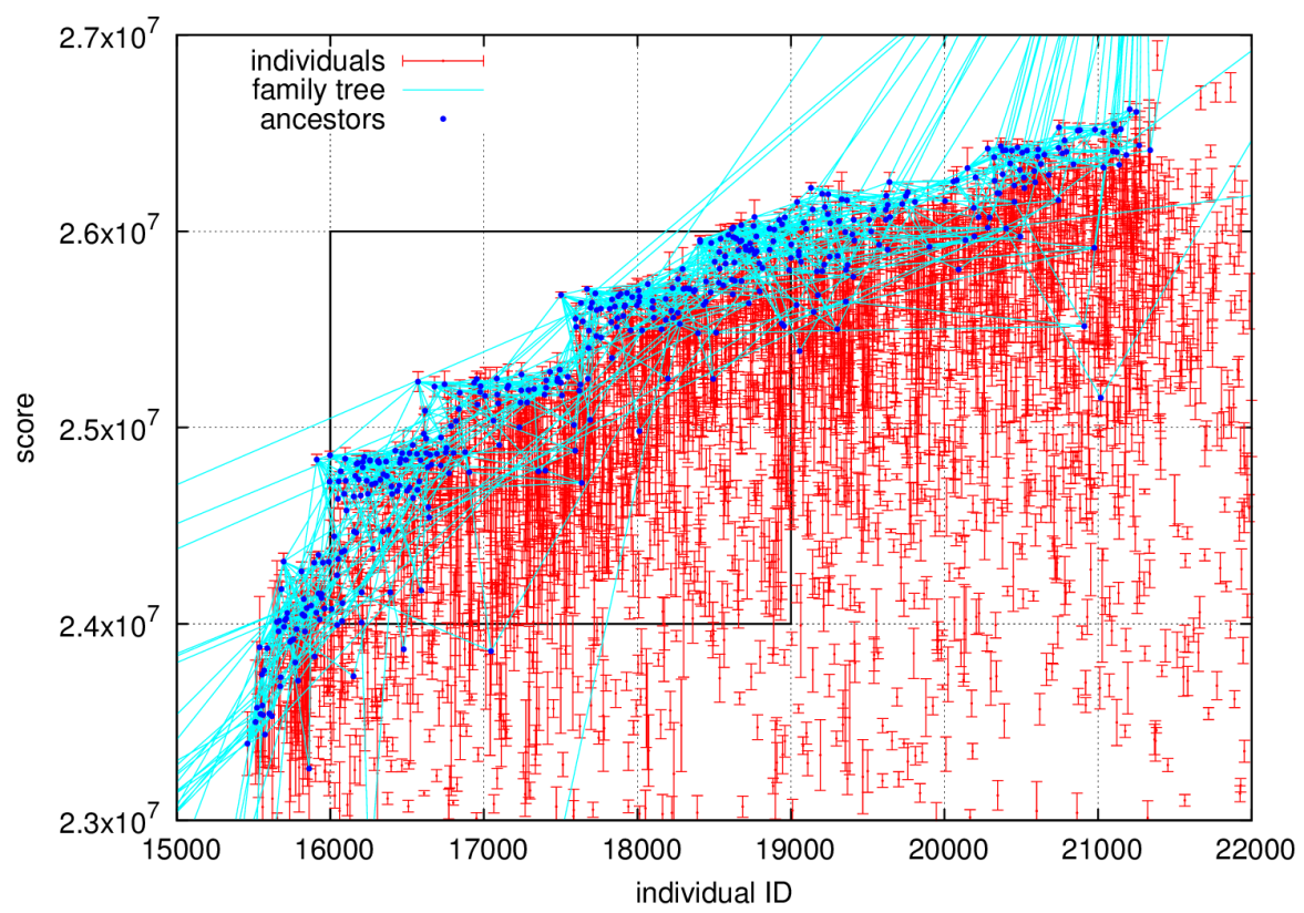
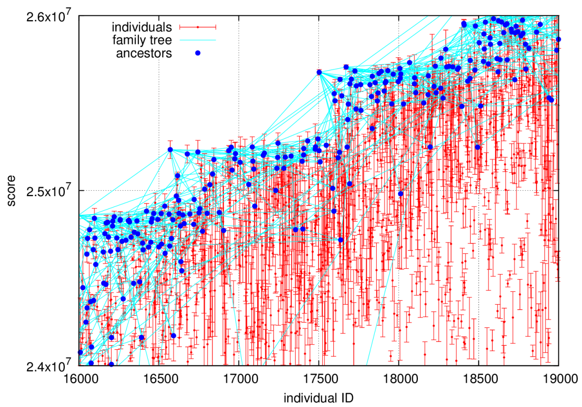
Figure 13: Two enlarged views of Fig. 11 showing $\mu(I)$ and $\sigma(I)$ as functions of $I$.

(a)	(b)

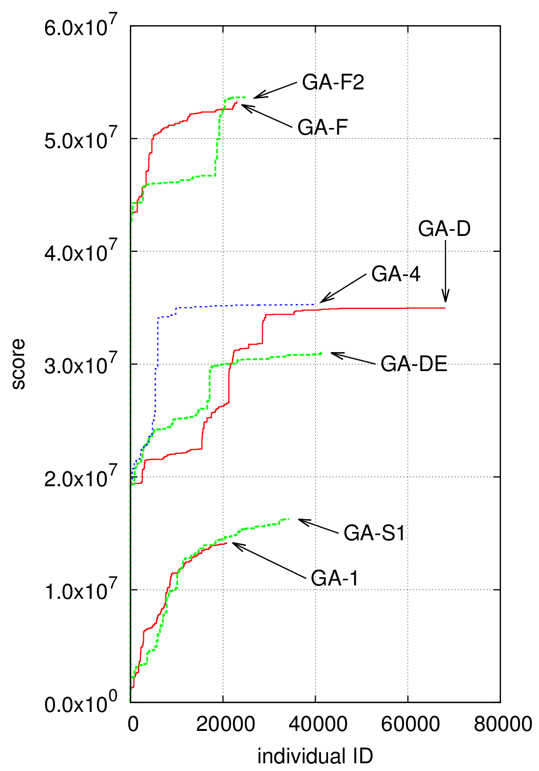
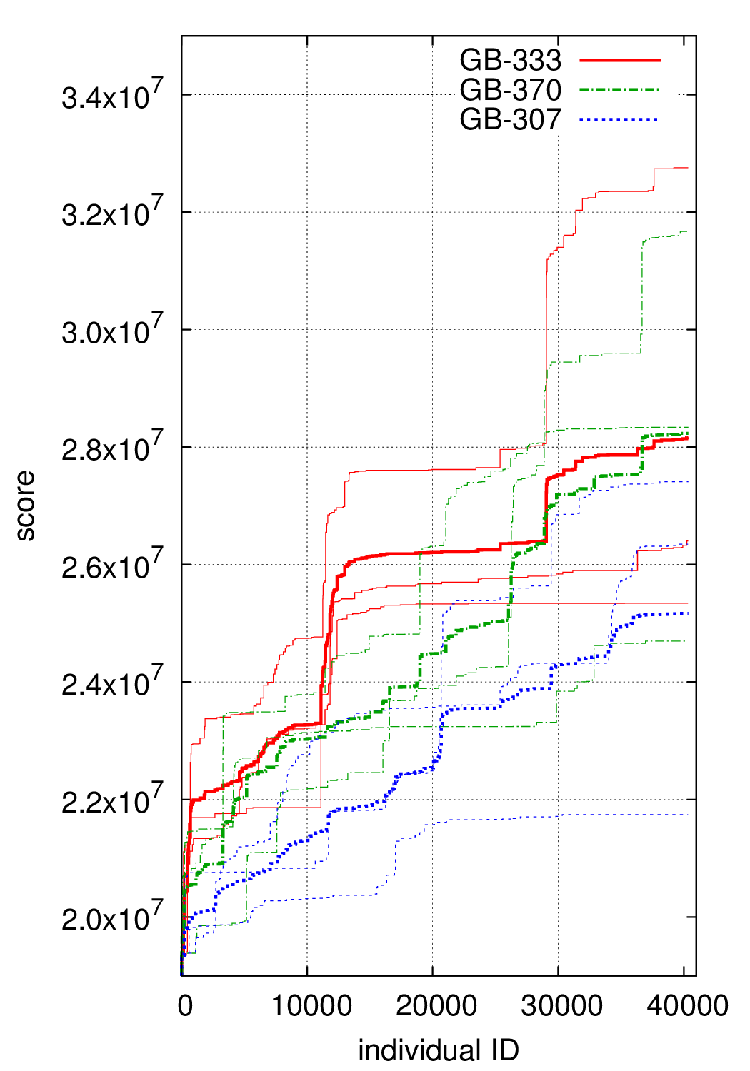
Figure 14: The evolution of the high score (in cups) as functions of ID in (a) experiments GA-* and (b) experiments GB-* . The three thick curves are the average of the GB-333-*, GB-370-* and GB-307-*, respectively. The average of GB-370-* was always higher than that of GB-307-*, and the average of GB-333-* was always higher than that of GB-370-* for the 89% of the time.

The functions of score against evolution progress exhibit self-similar structure of repeated cliff and plateau. For example, see the evolution history of experiment GA-D illustrated in Fig. 11 and its two enlarged views Fig. 12 and Fig. 13, with the family tree of the best individual superimposed. The evolution of the high scores in the experiments are shown in Fig. 14.

To design more efficient auto-tuning strategies, we investigate what have happened and which part of the evolution contributed to create better individuals in our automated tuning experiments. In section 5.2, we measure the contributions from three different tuning items. In section 5.3, we classify the individuals by their aspects such as their method of birth, their distance to the champion in the family tree, and their fitness relative to their parents. In section 5.4 we study how these classes contribute to the evolution by performing correlation analyses among these classes. In section 5.5, we study how the method of birth of parents affect their children. In section 5.6 we summarize and conclude the analyses.

ID	C	M	S	score(Mcups)	relative score	logscale
Izanagi	0	0	0	$1.137\pm 0.003$	$0.000\pm 0.000$	$0.000\pm 0.001$
	0	0	1	$1.122\pm 0.000$	$-0.001\pm 0.000$	$-0.005\pm 0.000$
	0	1	0	$5.400\pm 0.006$	$0.300\pm 0.000$	$0.599\pm 0.000$
	0	1	1	$5.300\pm 0.006$	$0.293\pm 0.000$	$0.591\pm 0.000$
	1	0	0	$3.073\pm 0.002$	$0.136\pm 0.000$	$0.382\pm 0.000$
	1	0	1	$2.946\pm 0.000$	$0.127\pm 0.000$	$0.366\pm 0.000$
	1	1	0	$15.829\pm 0.027$	$1.033\pm 0.002$	$1.012\pm 0.001$
GA-S1.33958	1	1	1	$15.354\pm 0.020$	$1.000\pm 0.001$	$1.000\pm 0.001$
Shinatsuhiko	0	0	0	$19.808\pm 0.033$	$0.000\pm 0.002$	$0.000\pm 0.003$
	0	0	1	$19.817\pm 0.030$	$0.001\pm 0.002$	$0.001\pm 0.003$
	0	1	0	$32.821\pm 0.058$	$0.848\pm 0.004$	$0.880\pm 0.003$
	0	1	1	$32.694\pm 0.057$	$0.839\pm 0.004$	$0.873\pm 0.003$
	1	0	0	$19.773\pm 0.050$	$-0.002\pm 0.003$	$-0.003\pm 0.004$
	1	0	1	$19.859\pm 0.058$	$0.003\pm 0.004$	$0.005\pm 0.005$
	1	1	0	$32.994\pm 0.273$	$0.859\pm 0.018$	$0.889\pm 0.014$
GA-4.33991	1	1	1	$35.160\pm 0.082$	$1.000\pm 0.005$	$1.000\pm 0.004$

Table 10: The score of the individuals created by artificial crossover between the initial individual $I_{0}$ and the best scoring individual $I_{\top}$. The second to fourth columns indicate which component was taken from which individual. Columns C,M,S correspond to CUDA kernel execution configuration, Manifest/Delay choice, synchronization timing, respectively. For each individual $I$ the fifth column shows $\mu(I)\pm\sigma(I)$, the sixth column shows $\displaystyle\frac{\mu(I)}{\mu(I_{\top})-\mu(I_{0})}\pm\frac{\sigma(I)}{\mu(I_{\top})-\mu(I_{0})}$ , and the seventh column shows $\displaystyle\frac{\log\mu(I)-\log\mu(I_{0})}{\log\mu(I_{\top})-\log\mu(I_{0})}$ $\displaystyle\pm\frac{\sigma(I)}{(\log\mu(I_{\top})-\log\mu(I_{0}))\mu(I)}$.

5.2 Contributions of The Three Genome Parts

We assign the symbols to genome parts with different functions as follows: (C): the CUDA kernel execution configuration, (M): which data to store on the memory (to make them Manifest), and (S): when to synchronize the computation. We first investigate how these three components contributed to the score by component-wise artificial crossover between the initial individual and the best scoring individual (Table 10). In the case of GA-S1.33958, introducing improvement only in C, M, S part increase the score by 14%, 30%, and 0%, respectively. In the case of GA-4.33991, the increase are 0%, 85%, 0%. Both cases exhibit synergy effect. Introducing several modifications simultaneously have more effect than the sum of the separate effects, they multiply. So addition in log-space explains 98% and 88% of the progress for GA-S1.33958 and GA-4.33991, respectively, but the score of the final individuals are still slightly higher than predicted.

Removing only one of C,M,S part from GA-4.33991 decreases the score by 16%, 100%, and 14%, respectively. Removing C,M,S part from GA-S1.33958 decreases the score by 71%, 87%, and $-3$%, respectively. Again we see the synergy effect, except that GA-S1.33958 were faster if S part were removed.

We conclude that the Manifest/Delayed trade-off plays the central part in improving the score. Fixing the Manifest/Delayed nodes, determines the decomposition of the data-flow graph. Then tuning the synchronization timing and CUDA kernel execution configuration help further improve the score.

5.3 Classifications of Individuals

To measure how each individual $I$ contributed in generating one of the best individuals, we define contribution distance $d(I)$, and classify the individuals to those who contributed to the evolution and those who didn’t. To begin with, let ${\mathbb{P}}(I)$ be the set of individual $I$’s parents. (we use $p$ for probability.) For individual $I$ born by mutation, crossover, and triangulation, the size of the parent set $n({\mathbb{P}}(I))$ is 1,2, and 3, respectively.

We define $d(I)$ as follows:

• $d(I_{\top})=0$ where $I_{\top}$ is the individual whose $\mu(I)$ was the largest in the history.

• $d(I)=0$ if $\mu(I)>\mu(I_{\top})-\sigma(I_{\top})$.

• $d(I)=0$ if one of $I$’s children $I_{c}$ satisfies $d(I_{c})=0$.

• $d(I)=1+\min\{d(I_{\mathbb{P}})|I_{\mathbb{P}}\in{\mathbb{P}}(I)\}$ otherwise.

We say that $I$ is one of the best individuals if $\mu(I)>\mu(I_{\top})-\sigma(I_{\top})$. For them, and their ancestors, $d(I)$ = 0. For other individuals $d(I)$ is the graph theoretical distance from the family trees of the best individuals. Table 12 - 18 shows the distributions of $d(I)$ for individuals born of mutation, crossover, and triangulation.

Next, we compare the fitness of the children with their parents. We classify the individuals into four ranks, namely $[\ll]$ , $[\leq]$ , $[\simeq]$ , and $[\gg]$ , based upon comparison of their scores with parents’ scores.

• $I\in$ $[\ll]$  if  $\forall I_{\mathrm{P}}\in{\mathbb{P}}(I):\mu(I)<\mu(I_{\mathrm{P}})-\sigma(I,I_{\mathrm{P}})$,

• $I\in$ $[\gg]$  if  $\forall I_{\mathrm{P}}\in{\mathbb{P}}(I):\mu(I)>\mu(I_{\mathrm{P}})+\sigma(I,I_{\mathrm{P}})$,

• $I\in$ $[\simeq]$  if  $|\mu(I)-\mu(I_{{\mathbb{P}}1})|<\sigma(I,I_{{\mathbb{P}}1})$ where $I_{{\mathbb{P}}1}$ is the member of ${\mathbb{P}}(I)$ with the largest $\mu$, and

• $I\in$ $[\leq]$ otherwise,

where $\sigma(I,I_{\mathrm{P}})\equiv(\sigma(I)^{2}+\sigma(I_{\mathrm{P}})^{2})^{0.5}$.

$[\gg]$ are children significantly faster than any of their parents; $[\simeq]$ are children whose scores are comparable to their fastest parents; $[\ll]$ are children significantly slower than any of their parents; and $[\leq]$ are children significantly slower than their best parent but not significantly slower than their slowest parents. Note that children of rank $[\leq]$ are never born by mutations since there is only one parent. Table 19 - 25 shows the classifications for experiments.

5.4 Chi-squared Tests of Correlations between Classes

To study which set of individuals are contributing to produce best species, we perform Pearson’s chi-squared test on pairs of predicates on individuals; see Table 26 and 27. We use $10^{-3}$ significance, or $X^{2}>10.83$ unless otherwise mentioned. Our observations are as follows:

• (row 1.) Significant negative correlations are detected between being born of mutation ($n({\mathbb{P}}(I))=1$) and being $d(I)=0$ for all experiments.

• (row 2.) Significant positive correlations are detected between being born of crossover ($n({\mathbb{P}}(I))=2$) and being $d(I)=0$ for all experiments but GA-S1.

• (row 3.) Significant positive correlations are detected between being born of triangulation ($n({\mathbb{P}}(I))=3$) and being $d(I)=0$ for all experiments.

• (row 4, 5.) Significant positive correlations are detected between being ($I\in{[\gg]}$) and being $d(I)=0$, and also between being ($I\in{[\simeq]}$) and being $d(I)=0$ for all experiments.

• (row 6.) Being ($I\in{[\leq]}$) and being $d(I)=0$ are negatively correlated for all experiments, but out of 10 experiments only 4 are $10^{-3}$ significant.

• (row 7.) Significant negative correlations are detected between being ($I\in{[\ll]}$) and being $d(I)=0$ for all experiments.

• (row 8, 9.) Within the population born of either crossover or triangulation, being born of triangulation ($n({\mathbb{P}}(I))=3$) and being $d(I)=0$ are still positively correlated for all experiments, but significant experiments are 7 out of 10.

• (row 10, 11.) Within the elite population ${\mathbb{E}}\equiv\{I|n({\mathbb{P}}(I))\geq 2\}\cap({[\gg]}\cup{[\simeq]})$, being ($I\in{[\gg]}$) and being $n({\mathbb{P}}(I))=2$ are significantly and positively correlated.

• (row 12-15.) Within the family tree of the champions $d(I)=0$, a subset of experiments shows that the pairs $(n({\mathbb{P}}(I))=2,I\in{[\gg]})$ and $(n({\mathbb{P}}(I))=3,I\in{[\simeq]})$ are positively correlated, and that the pairs $(n({\mathbb{P}}(I))=2,I\in{[\simeq]})$ and $(n({\mathbb{P}}(I))=3,I\in{[\gg]})$ are positively correlated. The number of significant examples are 7, 5, 2, and 7 out of 10, respectively, and no significant opposite correlation are observed.

• (row 16, 17.) Although 7 is considered to be a lucky number and 13 an unlucky number in Western culture, there is no correlation between having 7 at the lowest digit and being $d(I)=0$, nor having 13 as the two lowest digits and being $d(I)\neq 0$. These are control experiments.

5.5 Correlation along the Family Line

Next, we analyze the correlation along the family line by interpreting the family tree as Markov processes (c.f. Table 11). For each individual $I$ such that $d(I)=0$, we trace back its family tree in all possible ways for $n$ steps and obtain an $n$-letter word. For example, “312” means that $I$ is born of crossover, and one of its parent was born of mutation from an individual who was born of triangulation. With such bag of words obtained, we investigate how the last letter of a word is correlated with letters in front of them.

RunID	0th order	1st order	$2\to 2$	$3\to 3$	$22\to 2$	$33\to 3$
GA-1	2263.22	266.28	$\ominus 118.86$	$\oplus 1655.46$	$\oplus 32.54$	$\oplus 71.54$
GA-S1	1387.93	70.51	$\ominus 23.98$	$\oplus 1075.96$	$\ominus 5.19$	$\oplus 7.84$
GA-DE	546.42	43.31	$\oplus 3.34$	$\oplus 427.88$	$\ominus 9.85$	$\oplus 3.68$
GA-D	1038.15	88.20	$\ominus 42.78$	$\oplus 811.09$	$\oplus 3.90$	$\oplus 1.34$
GA-4	755.63	39.91	$\ominus 7.98$	$\oplus 580.33$	$\ominus 2.09$	$\ominus 2.60$
GA-F	422.08	22.24	$\ominus 2.07$	$\oplus 333.57$	$\oplus 0.96$	$\ominus 0.25$
GA-F2	490.90	86.34	$\ominus 23.63$	$\oplus 381.72$	$\oplus 16.29$	$\oplus 6.09$
GB-333-0	666.18	47.52	$\ominus 12.34$	$\oplus 511.62$	$\oplus 1.36$	$\ominus 2.52$
GB-333-1	930.33	25.26	$\ominus 48.06$	$\oplus 727.01$	$\ominus 0.86$	$\ominus 0.90$
GB-333-2	1208.20	68.11	$\ominus 39.34$	$\oplus 937.37$	$\oplus 0.34$	$\ominus 7.59$

Table 11: Chi-squared test of the family tree being lower-order Markov processes. The each column of the table shows the $X^{2}$ statistics of the null hypothesis the family tree being a $n$-th order Markov process and having no longer correlation.

The second columns show $X^{2}$ for null hypothesis “The bag of words is a 0th order Markov chain,” i.e. in the two-letter words the second letter is not correlated to the first. Formally written, the null hypothesis is:

$$p(ab)=p(a)p(b),$$ (69)

where $a$, $b$, $c$, … denote characters and $ab$, $abc$, … denote words.

The third columns show $X^{2}$ for null hypothesis “The bag of words is a 0th order Markov chain,” i.e. the probability of the occurrences of the letters depend only on their immediate predecessors and the distribution of three-letter words can be determined from the distribution of two-letter words. Formally written, the null hypothesis is:

$$p(abc)=\frac{p(ab)~{}p(bc)}{p(b)}.$$ (70)

Table 11 shows the result of the Markov chain analysis. Note that, the degree of freedom $k$ for 0th-order and 1st-order Markov chains are $4$ and $16$, respectively, and the chi-squared values for $10^{-3}$ significance are $X^{2}>18.47$ and $X^{2}>37.70$, respectively. From the table, we can deny the 0th-order Markov chain model for all of the experiments, and deny the 1st-order Markov chain model for 8 out of the 10 experiments. We also studied whether an occurence of a character is correlated to its prefix word. “3” was significantly likely to be followed by another “3” in all of the experiments, while “2” was significantly unlikely to be followed by another “2” in 6 out of 10 experiments. On the other hand, three consecutive occurences of the same letter was not significant at least in 8 out of 10 experiments.

5.6 Summary of The Analyses

Mutation is not efficient in directly producing individuals with good scores. Nevertheless mutations are indispensable part of the evolution because it is the only way that introduces new genomes to the genome pools and that have chance of finding new improvements.

Triangulations and crossover are two different methods to combine independently-found improvements, and are efficient in directly producing good individuals. Triangulations are relatively more efficient in producing $d(I)=0$ individuals. However, crossover is relatively good at making large jumps that belongs to $[\gg]$ . Triangulations are working in another way; the statistics indicate that one triangulation are likely to be followed by another triangulation in a family tree, and the sequence of Triangulations work to accumulate minor improvements that belongs to $[\simeq]$ to make a larger one. Fig. 14 — although the number of samples are too few to make a statistically significant statement — suggests that having both mode of combiner is better than having only one.

The main source of performance improvement was the change in memory layout and subroutine re-organization caused by making different Manifest/Delayed trade-offs. Tuning the synchronization timing and CUDA kernel execution configuration provided additional improvements.

The case of GA-S1.33958 is an evidence of the current genetic algorithm not finding the optimal individual. Random mutations tend to increase the genome entropy even under the selection pressure. Adding the rule-based mutations such as “remove all synchronization,” which are improbable under random mutations, may contribute to further optimization.

6 Conclusion and Discussion

We have designed and implemented Paraiso, a domain specific language for describing explicit solvers of partial differential equations, embedded in Haskell. Using the typelevel-tensor and algebraic type classes, we can explain our algorithms with simplicity of mathematical equations. Then the algorithm is translated to OpenMP code or CUDA code. The generated code can be optimized both by applying annotations by hand, and by automated tuning based on a genetic algorithm. Although we present just one example here — a second order Euler equations solver — the front end of Paraiso with typelevel-tensor and Builder Monad readily accept various other algorithms. The code generation and automated tuning can revolutionize the way we invent, implement and optimize various partial differential equation solvers.

The website of Paraiso is http://www.paraiso-lang.org/wiki/, where you can find codes, documentations, slides and videos.

Making more efficient searches for fast individuals is an important future extension of Paraiso. One way is to use machine learning, for example to make suggestions for genomes to introduce, or to predict the scores of the individuals before benchmarking them. Another approach is careful selection of the tuning items, importance of them given either by hand or by inference from the syntactic structure of Paraiso source code. The computing time invested in automated tuning is only justified if the optimized program is used repeatedly, or if optimized single-GPU program is used as a “core” of a multi-GPU program.

Making the automated tuning results more flexible and re-usable is another future challenge. For example, the size of the array e.g. $(N0,N1)$ in §2.2 for the two-dimensional OM, is fixed before native code generation under the current design of Paraiso. To change the size $N0$ or $N1$, the users need to re-run the code generation process. One solution is to improve the representation of the constant values in Paraiso, so that the users can set the values that are constant within a run but may vary across different runs. Possible examples of such constants include the OM size and the parameters of the algorithm.

On the other hand, the change in the dimension of the OM e.g. to three; $(N0,N1,N2)$, or the change in the algorithm described by the Builder Monad will change the number of nodes in the OM data flow graph and the bits in the genome. Therefore, the automatically tuned genomes before the change become useless. The genome must be redesigned to perform more re-usable, general automated tunings.

Generating codes for distributed computers / distributed and accelerated computers is another important future extension of Paraiso. To this end, instead of generating MPI codes by ourselves, we plan to generate parallel languages such as X10 [35], Chapel [36], and XcalableMP [15], or domain specific languages for stencil computations such as Physis [5].

Finally, the potential users and developers of Paraiso are obstructed by the programming language Haskell, which is a very computer-science language and is far from being mainstream in the fields of simulation science and high-performance computing. This is a disadvantage of Paraiso compared to other embedded DSL approaches based on more popular syntax such as Python (e.g. [37].) We make two remarks on this.

On the one hand, we show in this paper that abstract concepts developed by computer scientists and found in Haskell, is useful and was almost necessary in implementing a DSL that consistently handles the translation from mathematical notations to evolutionary computation. We hope that such powerful DSLs appear in many different fields, with help of the findings in computer science. On the other hand, we want many other researchers to become developers and users of Paraiso without requiring much knowledge in computer science.

For promotion of such development and use of Paraiso, we plan to provide interfaces to the code generation and the tuning stages in Paraiso, in terms of strings or in lightweight markup languages, along with their specifications. Those will allow many other programming languages can access those stages, such as OM data-flow graphs, their annotations, and the genomes. Adding a simulation scientist friendly scripting language layer on top of Builder Monad is another future work, so that people not familiar with Haskell can access Paraiso. We also plan to publish a series of tutorials and example programs in the Paraiso website. Such collaborations are fundamental to the realization of the future works listed in this section and computer-assisted programming in many fields of simulation science.

Appendix A supplementary data

$d(I)$	mutation	crossover	triangulation	total
0	1627(0.171)	1875(0.433)	3011(0.440)	6513(0.315)
1	4492(0.473)	1368(0.316)	2639(0.385)	8499(0.411)
2	2434(0.256)	944(0.218)	1129(0.165)	4507(0.218)
3	831(0.088)	141(0.033)	69(0.010)	1041(0.050)
4	104(0.011)	5(0.001)	2(0.000)	111(0.005)
5	6(0.001)	0(0.000)	0(0.000)	6(0.000)
6	1(0.000)	0(0.000)	0(0.000)	1(0.000)
sum	9495(1.000)	4333(1.000)	6850(1.000)	20678(1.000)

Table 12: Contribution distance analysis for experiment GA-1 : The numbers of individuals with specific $d(I)$ that is born of mutation, crossover, and triangulation. The last column shows the total numbers of individuals with specific $d(I)$. The decimal numbers inside the parentheses are the ratio of the number of individuals with specific $d(I)$ of specific birth, divided by total number of individuals of specific birth. Note that the grand total is slightly smaller than that in Table 7; this is because some worker nodes failed to write into DB.

$d(I)$	mutation	crossover	triangulation	total
0	1304(0.082)	915(0.106)	1411(0.145)	3631(0.106)
1	6136(0.386)	3601(0.416)	4696(0.481)	14433(0.421)
2	5461(0.344)	3211(0.371)	3161(0.324)	11833(0.345)
3	2392(0.151)	837(0.097)	470(0.048)	3699(0.108)
4	507(0.032)	79(0.009)	25(0.030)	611(0.018)
5	80(0.005)	7(0.001)	0(0.000)	87(0.003)
6	7(0.000)	0(0.000)	0(0.000)	7(0.000)
7	1(0.000)	0(0.000)	0(0.000)	1(0.000)
sum	15888(1.000)	8650(1.000)	9763(1.000)	34302(1.000)

Table 13: Contribution distance analysis for experiment GA-S1.

$d(I)$	mutation	crossover	triangulation	total
0	480(0.023)	430(0.047)	592(0.051)	1503(0.036)
1	10130(0.495)	4149(0.458)	6080(0.519)	20359(0.494)
2	6952(0.340)	3830(0.423)	4640(0.396)	15422(0.374)
3	2499(0.122)	622(0.069)	387(0.033)	3508(0.085)
4	385(0.019)	34(0.004)	12(0.001)	431(0.010)
5	21(0.001)	0(0.000)	0(0.000)	21(0.001)
6	4(0.000)	0(0.000)	0(0.000)	4(0.000)
7	1(0.000)	0(0.000)	0(0.000)	1(0.000)
sum	20472(1.000)	9065(1.000)	11711(1.000)	41249(1.000)

Table 14: Contribution distance analysis for experiment GA-DE.

$d(I)$	mutation	crossover	triangulation	total
0	785(0.023)	1099(0.071)	1680(0.087)	3565(0.052)
1	16113(0.482)	6208(0.403)	9699(0.503)	32020(0.470)
2	11510(0.344)	6946(0.451)	7490(0.389)	25946(0.381)
3	4509(0.135)	1139(0.074)	408(0.021)	6056(0.089)
4	472(0.014)	13(0.001)	1(0.000)	486(0.007)
5	21(0.001)	0(0.000)	0(0.000)	21(0.000)
6	2(0.000)	0(0.000)	0(0.000)	2(0.000)
sum	33412(1.000)	15405(1.000)	19278(1.000)	68096(1.000)

Table 15: Contribution distance analysis for experiment GA-D.

$d(I)$	mutation	crossover	triangulation	total
0	631(0.037)	730(0.066)	940(0.078)	2302(0.057)
1	7674(0.450)	5234(0.475)	6658(0.554)	19566(0.488)
2	6062(0.356)	4397(0.399)	4215(0.350)	14674(0.366)
3	2385(0.140)	644(0.058)	214(0.018)	3243(0.081)
4	291(0.017)	8(0.001)	0(0.000)	299(0.007)
5	9(0.001)	0(0.000)	0(0.000)	9(0.000)
sum	17052(1.000)	11013(1.000)	12027(1.000)	40093(1.000)

Table 16: Contribution distance analysis for experiment GA-4.

$d(I)$	mutation	crossover	triangulation	total
0	373(0.031)	329(0.068)	499(0.082)	1202(0.052)
1	6440(0.533)	2137(0.441)	3302(0.540)	11879(0.515)
2	3854(0.319)	2112(0.436)	2224(0.363)	8190(0.355)
3	1285(0.106)	262(0.054)	95(0.016)	1642(0.071)
4	137(0.011)	2(0.000)	0(0.000)	139(0.006)
5	4(0.000)	0(0.000)	0(0.000)	4(0.000)
sum	12093(1.000)	4842(1.000)	6120(1.000)	23056(1.000)

Table 17: Contribution distance analysis for experiment GA-F.

$d(I)$	mutation	crossover	triangulation	total
0	332(0.024)	314(0.076)	767(0.113)	1414(0.057)
1	7187(0.516)	1648(0.397)	3641(0.538)	12476(0.502)
2	4641(0.333)	1884(0.454)	2264(0.335)	8789(0.354)
3	1564(0.112)	295(0.071)	95(0.014)	1954(0.079)
4	190(0.014)	5(0.001)	0(0.000)	195(0.008)
5	21(0.002)	0(0.000)	0(0.000)	21(0.001)
sum	13935(1.000)	4146(1.000)	6767(1.000)	24849(1.000)

Table 18: Contribution distance analysis for experiment GA-F2.

mutation			crossover				triangulation
9437(1.000)			4335(1.000)				6834(1.000)
$[\ll]$	$[\simeq]$	$[\gg]$	$[\ll]$	$[\leq]$	$[\simeq]$	$[\gg]$	$[\ll]$	$[\leq]$	$[\simeq]$	$[\gg]$
7468	935	1022	934	1228	824	1347	976	2161	2420	1293
(0.787	0.098	0.108)	(0.216	0.283	0.190	0.311)	(0.142	0.315	0.353	0.189)
202	516	856	77	392	517	889	20	573	1593	825
(0.021	0.054	0.090)	(0.018	0.090	0.119	0.205)	(0.003	0.084	0.233	0.120)
0.027	0.552	0.838	0.082	0.319	0.627	0.660	0.020	0.265	0.658	0.638

Table 19: Children relative fitness for Experiment GA-1: The individuals classified based upon how they were born and their score with respect to their parents. For each class, the first row shows the number of individuals of that class, and the third row shows the number of individuals of that class with $d(I)=0$. The second and fourth rows are first and third row divided by the total number of individuals born in that way. The fifth row is the contribution ratio, the third row divided by the first row (or fourth divided by second).

mutation			crossover				triangulation
15887(1.000)			8655(1.000)				9758(1.000)
$[\ll]$	$[\simeq]$	$[\gg]$	$[\ll]$	$[\leq]$	$[\simeq]$	$[\gg]$	$[\ll]$	$[\leq]$	$[\simeq]$	$[\gg]$
9326	5818	743	1004	2868	4246	532	579	2427	6214	543
(0.587	0.366	0.047)	(0.116	0.332	0.491	0.062)	(0.059	0.249	0.636	0.056)
109	990	205	19	97	739	60	5	111	1190	105
(0.007	0.062	0.013)	(0.002	0.011	0.085	0.007)	(0.001	0.011	0.122	0.011)
0.012	0.170	0.276	0.019	0.034	0.174	0.113	0.009	0.046	0.192	0.193

Table 20: Children relative fitness classification for Experiment GA-S1.

mutation			crossover				triangulation
20473(1.000)			9064(1.000)				11711(1.000)
$[\ll]$	$[\simeq]$	$[\gg]$	$[\ll]$	$[\leq]$	$[\simeq]$	$[\gg]$	$[\ll]$	$[\leq]$	$[\simeq]$	$[\gg]$
16032	3273	1167	3082	876	3596	1511	3820	1386	4777	1728
(0.783	0.160	0.057)	(0.340	0.097	0.397	0.167)	(0.326	0.118	0.408	0.148)
89	328	63	33	30	298	69	28	49	446	69
(0.004	0.016	0.003)	(0.004	0.003	0.033	0.008)	(0.002	0.004	0.038	0.006)
0.006	0.100	0.054	0.011	0.034	0.083	0.046	0.007	0.035	0.093	0.040

Table 21: Children relative fitness classification for Experiment GA-DE.

mutation			crossover				triangulation
33420(1.000)			15412(1.000)				19261(1.000)
$[\ll]$	$[\simeq]$	$[\gg]$	$[\ll]$	$[\leq]$	$[\simeq]$	$[\gg]$	$[\ll]$	$[\leq]$	$[\simeq]$	$[\gg]$
30112	2510	788	4110	5694	4657	944	3899	8372	6382	625
(0.901	0.075	0.024)	(0.267	0.370	0.302	0.061)	(0.202	0.434	0.331	0.032)
420	313	52	122	204	648	125	90	370	1134	86
(0.013	0.009	0.002)	(0.008	0.013	0.042	0.008)	(0.005	0.019	0.059	0.004)
0.014	0.125	0.066	0.030	0.036	0.139	0.132	0.023	0.044	0.178	0.138

Table 22: Children relative fitness classification for Experiment GA-D.

mutation			crossover				triangulation
17054(1.000)			11015(1.000)				12017(1.000)
$[\ll]$	$[\simeq]$	$[\gg]$	$[\ll]$	$[\leq]$	$[\simeq]$	$[\gg]$	$[\ll]$	$[\leq]$	$[\simeq]$	$[\gg]$
13649	2791	606	3992	2849	3601	571	3523	3791	4318	395
(0.800	0.164	0.036)	(0.362	0.259	0.327	0.052)	(0.293	0.315	0.359	0.033)
217	363	51	96	97	459	78	69	161	654	56
(0.013	0.021	0.003)	(0.009	0.009	0.042	0.007)	(0.006	0.013	0.054	0.005)
0.016	0.130	0.084	0.024	0.034	0.127	0.137	0.020	0.042	0.151	0.142

Table 23: Children relative fitness classification for Experiment GA-4.

mutation			crossover				triangulation
12093(1.000)			4842(1.000)				6119(1.000)
$[\ll]$	$[\simeq]$	$[\gg]$	$[\ll]$	$[\leq]$	$[\simeq]$	$[\gg]$	$[\ll]$	$[\leq]$	$[\simeq]$	$[\gg]$
10569	1200	323	1744	1510	1300	288	1592	2528	1742	258
(0.874	0.099	0.027)	(0.360	0.312	0.268	0.059)	(0.260	0.413	0.285	0.042)
147	191	35	43	43	216	27	33	114	323	29
(0.012	0.016	0.003)	(0.009	0.009	0.045	0.006)	(0.005	0.019	0.053	0.005)
0.014	0.159	0.108	0.025	0.028	0.166	0.094	0.021	0.045	0.185	0.112

Table 24: Children relative fitness classification for Experiment GA-F.

mutation			crossover				triangulation
13933(1.000)			4151(1.000)				6759(1.000)
$[\ll]$	$[\simeq]$	$[\gg]$	$[\ll]$	$[\leq]$	$[\simeq]$	$[\gg]$	$[\ll]$	$[\leq]$	$[\simeq]$	$[\gg]$
12753	875	302	1286	1533	980	347	1705	3096	1765	201
(0.915	0.063	0.022)	(0.310	0.370	0.236	0.084)	(0.252	0.458	0.261	0.030)
203	103	26	30	68	173	43	63	198	461	45
(0.015	0.007	0.002)	(0.007	0.016	0.042	0.010)	(0.009	0.029	0.068	0.007)
0.016	0.118	0.086	0.023	0.044	0.177	0.124	0.037	0.064	0.261	0.224

Table 25: Children relative fitness classification for Experiment GA-F2.

	$f_{1}(I)$	$f_{2}(I)$	$f_{B}(I)$	GA-1	GA-S1	GA-DE	GA-D	GA-4	GA-F	GA-F2
1.	$n({\mathbb{P}}(I))=1$	$d(I)=0$	True	$1678.37\ominus$	$176.82\ominus$	$195.35\ominus$	$1101.14\ominus$	$228.43\ominus$	$233.27\ominus$	$646.90\ominus$
2.	$n({\mathbb{P}}(I))=2$	$d(I)=0$	True	$352.27\oplus$	$0.00\ominus$	$40.03\oplus$	$144.68\oplus$	$22.07\oplus$	$31.02\oplus$	$32.89\oplus$
3.	$n({\mathbb{P}}(I))=3$	$d(I)=0$	True	$736.92\oplus$	$215.63\oplus$	$92.78\oplus$	$656.16\oplus$	$136.57\oplus$	$145.75\oplus$	$552.01\oplus$
4.	$I\in{[\gg]}$	$d(I)=0$	True	$3086.23\oplus$	$193.47\oplus$	$11.85\oplus$	$172.65\oplus$	$109.81\oplus$	$50.53\oplus$	$97.78\oplus$
5.	$I\in{[\simeq]}$	$d(I)=0$	True	$2384.30\oplus$	$1766.64\oplus$	$1429.42\oplus$	$3566.00\oplus$	$1745.43\oplus$	$1513.70\oplus$	$1698.94\oplus$
6.	$I\in{[\leq]}$	$d(I)=0$	True	$8.22\ominus$	$291.79\ominus$	$0.08\ominus$	$47.13\ominus$	$50.13\ominus$	$16.82\ominus$	$0.05\oplus$
7.	$I\in{[\ll]}$	$d(I)=0$	True	$6373.92\ominus$	$1482.62\ominus$	$1314.95\ominus$	$2233.94\ominus$	$1283.65\ominus$	$923.74\ominus$	$1162.42\ominus$
8.	$n({\mathbb{P}}(I))=2$	$d(I)=0$	$n({\mathbb{P}}(I))\geq 2$	$0.50\ominus$	$62.38\ominus$	$1.06\ominus$	$29.02\ominus$	$12.05\ominus$	$7.15\ominus$	$40.75\ominus$
9.	$n({\mathbb{P}}(I))=3$	$d(I)=0$	$n({\mathbb{P}}(I))\geq 2$	$0.50\oplus$	$62.38\oplus$	$1.06\oplus$	$29.02\oplus$	$12.05\oplus$	$7.15\oplus$	$40.75\oplus$
10.	$n({\mathbb{P}}(I))=2$	$I\in{[\gg]}$	$I\in{\mathbb{E}}$	$410.39\oplus$	$31.79\oplus$	$13.00\oplus$	$179.86\oplus$	$64.28\oplus$	$18.81\oplus$	$144.85\oplus$
11.	$n({\mathbb{P}}(I))=3$	$I\in{[\gg]}$	$I\in{\mathbb{E}}$	$410.39\ominus$	$31.79\ominus$	$13.00\ominus$	$179.86\ominus$	$64.28\ominus$	$18.81\ominus$	$144.85\ominus$
12.	$n({\mathbb{P}}(I))=2$	$I\in{[\gg]}$	$d(I)=0$	$69.73\oplus$	$17.64\ominus$	$3.72\oplus$	$37.14\oplus$	$10.15\oplus$	$0.26\oplus$	$17.27\oplus$
13.	$n({\mathbb{P}}(I))=2$	$I\in{[\simeq]}$	$d(I)=0$	$177.77\ominus$	$0.11\oplus$	$1.20\ominus$	$0.03\oplus$	$0.72\ominus$	$4.60\oplus$	$1.43\oplus$
14.	$n({\mathbb{P}}(I))=3$	$I\in{[\gg]}$	$d(I)=0$	$340.94\ominus$	$19.05\ominus$	$2.49\ominus$	$23.71\ominus$	$9.29\ominus$	$3.77\ominus$	$10.90\ominus$
15.	$n({\mathbb{P}}(I))=3$	$I\in{[\simeq]}$	$d(I)=0$	$368.68\oplus$	$22.80\oplus$	$7.69\oplus$	$100.03\oplus$	$20.56\oplus$	$5.72\oplus$	$42.80\oplus$
16.	$I\equiv 7\ \mathrm{mod}\ 10$	$d(I)=0$	True	$1.73\ominus$	$1.38\ominus$	$0.41\ominus$	$1.00\ominus$	$0.98\oplus$	$0.00\ominus$	$0.02\ominus$
17.	$I\equiv 13\ \mathrm{mod}\ 100$	$d(I)=0$	True	$1.05\oplus$	$0.69\oplus$	$0.06\oplus$	$0.08\ominus$	$0.43\ominus$	$0.08\oplus$	$1.11\oplus$

Table 26: Chi-squared test of statistical independence of predicates. For each pair of experiment (columns) and three predicates $f_{1}(I),f_{2}(I),f_{B}(I)$, the table shows the $X^{2}$ statistics of the null hypothesis “predicates $f_{1}(I)$ and $f_{2}(I)$ are statistically independent for the population of individuals that satisfy predicate $f_{B}(I)$. ” Here, ${\mathbb{E}}\equiv\{I|n({\mathbb{P}}(I))\geq 2\}\cap({[\gg]}\cup{[\simeq]})$. $\oplus$ denotes the positive correlation and $\ominus$ denotes the negative correlation.

	$f_{1}(I)$	$f_{2}(I)$	$f_{B}(I)$	GB-333-0	GB-333-1	GB-333-2
1.	$n({\mathbb{P}}(I))=1$	$d(I)=0$	True	$189.24\ominus$	$309.78\ominus$	$374.03\ominus$
2.	$n({\mathbb{P}}(I))=2$	$d(I)=0$	True	$17.50\oplus$	$1.38\oplus$	$15.90\oplus$
3.	$n({\mathbb{P}}(I))=3$	$d(I)=0$	True	$107.73\oplus$	$284.28\oplus$	$255.24\oplus$
4.	$I\in{[\gg]}$	$d(I)=0$	True	$19.56\oplus$	$28.84\oplus$	$41.97\oplus$
5.	$I\in{[\simeq]}$	$d(I)=0$	True	$455.57\oplus$	$517.15\oplus$	$1024.86\oplus$
6.	$I\in{[\leq]}$	$d(I)=0$	True	$0.05\ominus$	$1.67\ominus$	$8.49\ominus$
7.	$I\in{[\ll]}$	$d(I)=0$	True	$333.89\ominus$	$514.23\ominus$	$794.08\ominus$
8.	$n({\mathbb{P}}(I))=2$	$d(I)=0$	$n({\mathbb{P}}(I))\geq 2$	$9.69\ominus$	$67.58\ominus$	$38.17\ominus$
9.	$n({\mathbb{P}}(I))=3$	$d(I)=0$	$n({\mathbb{P}}(I))\geq 2$	$9.69\oplus$	$67.58\oplus$	$38.17\oplus$
10.	$n({\mathbb{P}}(I))=2$	$I\in{[\gg]}$	$I\in{\mathbb{E}}$	$207.54\oplus$	$70.91\oplus$	$138.99\oplus$
11.	$n({\mathbb{P}}(I))=3$	$I\in{[\gg]}$	$I\in{\mathbb{E}}$	$207.54\ominus$	$70.91\ominus$	$138.99\ominus$
12.	$n({\mathbb{P}}(I))=2$	$I\in{[\gg]}$	$d(I)=0$	$43.23\oplus$	$12.05\oplus$	$70.57\oplus$
13.	$n({\mathbb{P}}(I))=2$	$I\in{[\simeq]}$	$d(I)=0$	$1.47\oplus$	$17.39\ominus$	$0.22\ominus$
14.	$n({\mathbb{P}}(I))=3$	$I\in{[\gg]}$	$d(I)=0$	$44.86\ominus$	$18.46\ominus$	$60.99\ominus$
15.	$n({\mathbb{P}}(I))=3$	$I\in{[\simeq]}$	$d(I)=0$	$3.15\oplus$	$7.75\oplus$	$0.12\ominus$
16.	$I\equiv 7\ \mathrm{mod}\ 10$	$d(I)=0$	True	$3.77\ominus$	$0.47\oplus$	$2.74\oplus$
17.	$I\equiv 13\ \mathrm{mod}\ 100$	$d(I)=0$	True	$0.63\ominus$	$4.27\ominus$	$0.23\ominus$

Table 27: The same table for GB-333-*.

References

References

- [1] M. Frigo and S.G. Johnson. The design and implementation of FFTW3. Proceedings of the IEEE, 93(2):216–231, 2005.
- [2] R. Clint Whaley, A. Petitet, and J.J. Dongarra. Automated empirical optimizations of software and the ATLAS project. Parallel Computing, 27(1-2):3–35, 2001.
- [3] M. Puschel, J.M.F. Moura, J.R. Johnson, D. Padua, M.M. Veloso, B.W. Singer, J. Xiong, F. Franchetti, A. Gacic, Y. Voronenko, et al. SPIRAL: code generation for DSP transforms. Proceedings of the IEEE, 93(2):232–275, 2005.
- [4] Kaushik Datta, Mark Murphy, Vasily Volkov, Samuel Williams, Jonathan Carter, Leonid Oliker, David Patterson, John Shalf, and Katherine Yelick. Stencil computation optimization and auto-tuning on state-of-the-art multicore architectures. In Proceedings of the 2008 ACM/IEEE conference on Supercomputing, SC ’08, page 4:1–4:12, Piscataway, NJ, USA, 2008. IEEE Press.
- [5] Naoya Maruyama, Tatsuo Nomura, Kento Sato, and Satoshi Matsuoka. Physis: an implicitly parallel programming model for stencil computations on large-scale GPU-accelerated supercomputers. In Proceedings of 2011 International Conference for High Performance Computing, Networking, Storage and Analysis, SC ’11, page 11:1–11:12, New York, NY, USA, 2011. ACM.
- [6] P.W. Trinder, H.W. Loidl, and R.F. Pointon. Parallel and distributed haskells. Journal of Functional Programming, 12(5):469–510, 2002.
- [7] M. Chakravarty, G. Keller, R. Lechtchinsky, and W. Pfannenstiel. Nepal—nested data parallelism in haskell. Euro-Par 2001 Parallel Processing, page 524–534, 2001.
- [8] S.P. Jones, R. Leshchinskiy, G. Keller, and M.M.T. Chakravarty. Harnessing the multicores: Nested data parallelism in haskell. In FSTTCS, volume 2, page 383–414, 2008.
- [9] M.M.T. Chakravarty, G. Keller, S. Lee, T.L. McDonell, and V. Grover. Accelerating haskell array codes with multicore GPUs. In Proceedings of the sixth workshop on Declarative aspects of multicore programming, page 3–14, 2011.
- [10] G. Mainland and G. Morrisett. Nikola: embedding compiled GPU functions in haskell. In Proceedings of the third ACM Haskell symposium on Haskell, page 67–78, 2010.
- [11] Zachary DeVito, Niels Joubert, Francisco Palacios, Stephen Oakley, Montserrat Medina, Mike Barrientos, Erich Elsen, Frank Ham, Alex Aiken, Karthik Duraisamy, Eric Darve, Juan Alonso, and Pat Hanrahan. Liszt: a domain specific language for building portable mesh-based PDE solvers. In Proceedings of 2011 International Conference for High Performance Computing, Networking, Storage and Analysis, SC ’11, page 9:1–9:12, New York, NY, USA, 2011. ACM.
- [12] Takashi Shimokawabe, Takayuki Aoki, Chiashi Muroi, Junichi Ishida, Kohei Kawano, Toshio Endo, Akira Nukada, Naoya Maruyama, and Satoshi Matsuoka. An 80-Fold speedup, 15.0 TFlops full GPU acceleration of Non-Hydrostatic weather model ASUCA production code. In Proceedings of the 2010 ACM/IEEE International Conference for High Performance Computing, Networking, Storage and Analysis, SC ’10, page 1–11, Washington, DC, USA, 2010. IEEE Computer Society.
- [13] Takashi Shimokawabe, Takayuki Aoki, Tomohiro Takaki, Toshio Endo, Akinori Yamanaka, Naoya Maruyama, Akira Nukada, and Satoshi Matsuoka. Peta-scale phase-field simulation for dendritic solidification on the TSUBAME 2.0 supercomputer. In Proceedings of 2011 International Conference for High Performance Computing, Networking, Storage and Analysis, SC ’11, page 3:1–3:11, New York, NY, USA, 2011. ACM.
- [14] T. Hoshino, H.S. Stone, and S. Goldman. PAX Computer; High-Speed Parallel Processing and Scientific Computing. Addison-Wesley Longman Publishing Co., Inc., 1989.
- [15] J. Lee and M. Sato. Implementation and performance evaluation of xcalablemp: A parallel programming language for distributed memory systems. In Parallel Processing Workshops (ICPPW), 2010 39th International Conference on, page 413–420, 2010.
- [16] C. McBride and R. Paterson. Functional pearl: Applicative programming with effects. Journal of functional programming, 18(1):1–13, 2008.
- [17] G. Keller, M.M.T. Chakravarty, R. Leshchinskiy, S. Peyton Jones, and B. Lippmeier. Regular, shape-polymorphic, parallel arrays in haskell. ACM SIGPLAN Notices, 45(9):261–272, 2010.
- [18] J. Gibbons and B.C.S. Oliveira. The essence of the iterator pattern. Journal of Functional Programming, 19(3-4):377–402, 2009.
- [19] M. Erwig. Functional programming with graphs. In ACM SIGPLAN Notices, volume 32, page 52–65, 1997.
- [20] M. Erwig. Inductive graphs and functional graph algorithms. Journal of Functional Programming, 11(05):467–492, 2001.
- [21] T. Sheard and S.P. Jones. Template meta-programming for haskell. In Proceedings of the 2002 ACM SIGPLAN workshop on Haskell, page 1–16, 2002.
- [22] Dylan Thurston, Henning Thielemann, and Mikael Johansson. numeric-prelude: An experimental alternative hierarchy of numeric type classes. http://hackage.haskell.org/package/numeric-prelude, 2012.
- [23] Ralf Lämmel and Simon Peyton Jones. Scrap your boilerplate: a practical design pattern for generic programming. SIGPLAN Not., 38(3):26–37, January 2003.
- [24] Koji Hukushima and Koji Nemoto. Exchange monte carlo method and application to spin glass simulations. Journal of the Physical Society of Japan, 65:1604–1608, 1996.
- [25] José A. García Gutiérrez, Carlos Cotta, and Antonio J Fernández-Leiva. Evolutionary computation in astronomy and astrophysics: A review. arXiv:1202.2523, February 2012.
- [26] A. Eiben, P. Raué, and Z. Ruttkay. Genetic algorithms with multi-parent recombination. Parallel Problem Solving from Nature—PPSN III, page 78–87, 1994.
- [27] SN Sivanandam and SN Deepa. Introduction to genetic algorithms. Springer Verlag, 2007.
- [28] A. Eiben, C. Van Kemenade, and J. Kok. Orgy in the computer: Multi-parent reproduction in genetic algorithms. Advances in Artificial Life, page 934–945, 1995.
- [29] S. Tsutsui, M. Yamamura, and T. Higuchi. Multi-parent recombination with simplex crossover in real coded genetic algorithms. In Proceedings of the Genetic and Evolutionary Computation Conference, volume 1, page 657–664, 1999.
- [30] Eleuterio F. Toro. Riemann Solvers And Numerical Methods for Fluid Dynamics: A Practical Introduction. Springer-Verlag, 3 edition, June 2009.
- [31] P.K. Sweby. High resolution schemes using flux limiters for hyperbolic conservation laws. SIAM journal on numerical analysis, page 995–1011, 1984.
- [32] E. F. Toro, M. Spruce, and W. Speares. Restoration of the contact surface in the HLL-Riemann solver. Shock Waves, 4(1):25–34, July 1994.
- [33] H.Y. Schive, U.H. Zhang, and T. Chiueh. Directionally unsplit hydrodynamic schemes with hybrid MPI/OpenMP/GPU parallelization in AMR. Arxiv preprint arXiv:1103.3373, 2011.
- [34] M. de la Asuncióna, M.J. Castroc, ED Fernández-Nietob, J.M. Mantasa, S.O. Acostac, and J.M. González-Vidad. Efficient GPU implementation of a two waves WAF method for the two-dimensional one layer shallow water system on structured meshes.
- [35] Philippe Charles, Christian Grothoff, Vijay Saraswat, Christopher Donawa, Allan Kielstra, Kemal Ebcioglu, Christoph von Praun, and Vivek Sarkar. X10: an object-oriented approach to non-uniform cluster computing. SIGPLAN Not., 40(10):519–538, October 2005.
- [36] B.l. Chamberlain, D. Callahan, and H.p. Zima. Parallel programmability and the chapel language. International Journal of High Performance Computing Applications, 21(3):291 –312, 2007.
- [37] Jon K Nilsen, Xing Cai, Bjørn Høyland, and Hans Petter Langtangen. Simplifying the parallelization of scientific codes by a function-centric approach in python. Computational Science & Discovery, 3(1):015003, September 2010.