NLO QCD corrections to dijet production via quark contact interactions

Abstract

We present the exact next-to-leading order (NLO) QCD corrections to dijet production at the LHC via quark contact interactions, with different color and chiral structures induced from new physics. Following the recent analysis of quark compositeness search at the LHC, we find that the NLO QCD corrections can lower the dijet cross sections by several tens percent, depending on the theory parameters and the selected kinematic regions, and reduce the dependence of the cross sections on factorization and renormalization scales. We also calculate the renormalization group (RG) improved NLO cross sections by summing over the large logarithms from the RG running of Wilson coefficients. Moreover, we investigate the NLO QCD effects on various experimental observables and exclusion limits of quark compositeness scale.

1 Introduction

Jet production at hadron colliders provides an excellent opportunity to test perturbative QCD (PQCD) and to search for possible new physics (NP) beyond the Standard Model (SM) over a wide range of energy scales. Invariant mass distributions of the dijets Chatrchyan:2011ns , the dijet angular distributions Khachatryan:2011as ; Aad:2011aj ; Chatrchyan:2012bf , and other jet observables at the LHC :2010wv have already extended current searches for quark compositeness, excited quarks, and other new particle resonances toward the highest energies attainable. Among all these measurements, the dijet angular distribution shows a great sensitivity to possible quark contact interactions induced by new physics models. In the SM, Quantum Chromodynamics (QCD) predicts the jets in dijet events are preferably produced in large rapidity region, via small angle scattering in t-channel processes. On the contrary, the dijet angular distribution induced by quark contact interactions is expected to be much more isotropic, and thus the dijet angular distribution at the LHC could be largely modified.

The measurement of quark contact interactions has been used to set limits on the quark composite models which have been studied extensively in the literature Eichten:1983hw ; Lane:1996gr . It is assumed that quarks are composed of more fundamental particles with new strong interactions at a compositeness scale $\Lambda$, much greater than the quark mass scales. At the energy well below $\Lambda$, quark contact interactions are induced by the underlying strong dynamics, and yield observable signals at hadron colliders. The newest bounds of $\Lambda$ at the $95\%$ confidence level (C.L.) from the CMS collaboration are around $10\,{\rm TeV}$ Chatrchyan:2012bf based on $2.2\,{\rm fb}^{-1}$ collected data. Previous limits from the Tevatron and LHC can be found in Refs. Khachatryan:2011as ; Aad:2011aj ; Abe:1996mj ; Collaboration:2010eza . With more integrated luminosity collected, these limits will be further improved.

In our previous work Gao:2011ha , we carried out the next-to-leading order (NLO) QCD correction for dijet production at the LHC induced by the quark contact interactions that are the products of left-handed electroweak isoscalar quark currents. We compared it with the leading order (LO) results used by the CMS Collaboration and also the “scaled NLO results” used by the ATLAS Collaboration, which assumes the NLO correction (in terms of K-factors, defined as the ratio of NLO cross sections to LO ones) to the dijet production from contact interactions to be exactly the same as that from the SM QCD interactions. And we derived, based on our exact NLO results, the corrected limits of compositeness scale for the CMS and ATLAS measurements with $3\,{\rm pb}^{-1}$ data Collaboration:2010eza . In this paper, we extend our previous work to include more quark contact interaction operators in the NLO QCD calculations, which allows the mixing of operators with different chiral structures at the NLO level, and show more details of the calculations. The effect of our results to measurements of quark compositeness at the LHC is also investigated. In the appendix, we discuss some details of our numerical code developed for the calculations presented in this paper.

2 Theoretical setup

We consider a subset of quark contact interactions that are the products of electroweak isoscalar quark currents which are assumed to be flavor-symmetric to avoid large flavor-changing neutral-current interactions Lane:1996gr . The effective Lagrangian can be written as

$$\mathcal{L}_{NP}=\frac{1}{2\Lambda^{2}}\sum_{i=1}^{6}c_{i}O_{i},$$ (1)

where $\Lambda$ is the new physics scale, $c_{i}$ are Wilson coefficients. And the operators $O_{i}$ in chiral basis are given by

$$O_{1} = \delta_{ij}\delta_{kl}\left(\sum_{c=1}^{3}\bar{q}_{Lci}\gamma_{\mu}q_{Lcj}\sum_{d=1}^{3}\bar{q}_{Ldk}\gamma^{\mu}q_{Ldl}\right),$$

$$O_{2} = {\rm T}_{ij}^{a}{\rm T}_{kl}^{a}\left(\sum_{c=1}^{3}\bar{q}_{Lci}\gamma_{\mu}q_{Lcj}\sum_{d=1}^{3}\bar{q}_{Ldk}\gamma^{\mu}q_{Ldl}\right),$$

$$O_{3} = \delta_{ij}\delta_{kl}\left(\sum_{c=1}^{3}\bar{q}_{Lci}\gamma_{\mu}q_{Lcj}\sum_{d=1}^{3}\bar{q}_{Rdk}\gamma^{\mu}q_{Rdl}\right),$$

$$O_{4} = {\rm T}_{ij}^{a}{\rm T}_{kl}^{a}\left(\sum_{c=1}^{3}\bar{q}_{Lci}\gamma_{\mu}q_{Lcj}\sum_{d=1}^{3}\bar{q}_{Rdk}\gamma^{\mu}q_{Rdl}\right),$$

$$O_{5} = \delta_{ij}\delta_{kl}\left(\sum_{c=1}^{3}\bar{q}_{Rci}\gamma_{\mu}q_{Rcj}\sum_{d=1}^{3}\bar{q}_{Rdk}\gamma^{\mu}q_{Rdl}\right),$$

$$O_{6} = {\rm T}_{ij}^{a}{\rm T}_{kl}^{a}\left(\sum_{c=1}^{3}\bar{q}_{Rci}\gamma_{\mu}q_{Rcj}\sum_{d=1}^{3}\bar{q}_{Rdk}\gamma^{\mu}q_{Rdl}\right),$$ (2)

in which $c$, $d$ are generation indices and $i$, $j$, $k$, $l$, $a$ are color indices, and ${\rm T}^{a}$ are the Gell-Mann matrices with the normalization ${\rm Tr}({\rm T}^{a}{\rm T}^{b})=\delta^{ab}/2$. Beside of the quark compositeness, the above interactions can also arise from various kinds of new physics models, induced by the exchange of new heavy resonances, such as $Z^{\prime}$ models Langacker:2008yv and extra dimensions models Randall:1999ee . Thus our analyses here are rather model independent and $\Lambda$ can be identified as the effective new physics (NP) scale.

The above six operators have been extensively studied in weak decays of mesons Buchalla:1995vs . They mix with each other through QCD loop diagrams, which requires a renormalization matrix of the operators to cancel all the ultraviolet divergences, defined by $O_{i}^{(0)}=(1+\delta Z)_{ij}O_{j}$. After calculating one-loop diagrams, to be shown latter, with the dimensional regularization scheme in $n=4-2\epsilon$ dimensions, we obtain the matrix at the NLO as follow

$$\delta Z=D_{\epsilon}{\alpha_{s}\over 4\pi}{1\over\epsilon}\left(\begin{array}[]{cccccc}0&-{22\over 3}&0&-{4\over 3}&0&0\\ -{3C_{F}\over N}&{20\over 3N}-{2\over 3}n_{f}&0&{2\over 3N}-{2\over 3}n_{f}&0&0\\ 0&0&0&6&0&0\\ 0&-{n_{f}\over 3}&{3C_{F}\over N}&6C_{F}-{3\over N}-{2\over 3}n_{f}&0&-{n_{f}\over 3}\\ 0&0&0&-{4\over 3}&0&-{22\over 3}\\ 0&0&0&{2\over 3N}-{2\over 3}n_{f}&-{3C_{F}\over N}&{20\over 3N}-{2\over 3}n_{f}\\ \end{array}\right),$$ (3)

where$D_{\epsilon}=\frac{(4\pi)^{\epsilon}}{\Gamma(1-\epsilon)}$, $N=3$ and $C_{F}=4/3$ for QCD, and $n_{f}=5$ is the activate quark numbers in the loop. (Here, we do not include the top quark contribution in the loops).

3 Analytical results

3.1 NLO corrections

At LO, there are several subprocesses which contribute to the dijet production at hadron colliders induced by the operators under consideration. They are

$$qq^{\prime}(q)\rightarrow qq^{\prime}(q),\ q\bar{q}^{\prime}\rightarrow q\bar{q}^{\prime},\ q\bar{q}\rightarrow q\bar{q}(q^{\prime}\bar{q}^{\prime}),$$ (4)

where $q$, $q^{\prime}$ could be all the light quarks except the top quark. The NP contributions included in our calculation consist of two parts, the NP squared terms and the interference terms between the NP and the SM QCD interactions, which have different behavior with the increase of dijet invariant mass. We carried out the NLO calculations in the Feynman-’t Hooft gauge with dimensional regularization (DR) scheme (with naive $\gamma_{5}$ prescription) Buchalla:1995vs in $n=4-2\epsilon$ dimensions to regularize all the divergences. Below, we only show the analytical results for the subprocess $q(p_{1})q^{\prime}(p_{2})\rightarrow q(p_{3})q^{\prime}(p_{4})$, since the similar results for other subprocesses can be obtained by crossing symmetry.

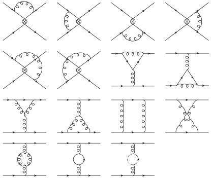
Figure 1: Loop diagrams for both the SM QCD and NP contributions to $qq^{\prime}\to qq^{\prime}$ at the NLO.

First, we define the following abbreviations for color structures and matrix elements,

$$\mathcal{M}_{1} = \bar{u}_{L}(p_{3})\gamma_{\mu}u_{L}(p_{1})\bar{u}_{L}(p_{4})\gamma^{\mu}u_{L}(p_{2}),$$

$$\mathcal{M}_{2} = \bar{u}_{R}(p_{3})\gamma_{\mu}u_{R}(p_{1})\bar{u}_{R}(p_{4})\gamma^{\mu}u_{R}(p_{2}),$$

$$\mathcal{M}_{3} = (\bar{u}_{L}(p_{3})\gamma_{\mu}u_{L}(p_{1})\bar{u}_{R}(p_{4})\gamma^{\mu}u_{R}(p_{2})$$

$$+\bar{u}_{R}(p_{3})\gamma_{\mu}u_{R}(p_{1})\bar{u}_{L}(p_{4})\gamma^{\mu}u_{L}(p_{2}))/2,$$

$$\mathcal{C}_{1} = \delta_{i_{3}i_{1}}\delta_{i_{4}i_{2}},\ \mathcal{C}_{2}={\rm T}_{i_{3}i_{1}}^{a}{\rm T}_{i_{4}i_{2}}^{a},$$ (5)

where $i_{1-4}$ are the color indices of the external quarks. The LO scattering amplitudes induced by the NP and the SM QCD interactions can be separately written as

$$i\mathcal{M}_{NP,1}^{tree} = i\mathcal{M}_{1}(c_{1}\mathcal{C}_{1}+c_{2}\mathcal{C}_{2})/\Lambda^{2},$$

$$i\mathcal{M}_{NP,2}^{tree} = i\mathcal{M}_{2}(c_{5}\mathcal{C}_{1}+c_{6}\mathcal{C}_{2})/\Lambda^{2},$$

$$i\mathcal{M}_{NP,3}^{tree} = i\mathcal{M}_{3}(c_{3}\mathcal{C}_{1}+c_{4}\mathcal{C}_{2})/\Lambda^{2},$$

$$i\mathcal{M}_{SM,1}^{tree} = i\mathcal{M}_{1}(4\pi\alpha_{s}\mathcal{C}_{2})/t,$$

$$i\mathcal{M}_{SM,2}^{tree} = i\mathcal{M}_{2}(4\pi\alpha_{s}\mathcal{C}_{2})/t,$$

$$i\mathcal{M}_{SM,3}^{tree} = i\mathcal{M}_{3}(8\pi\alpha_{s}\mathcal{C}_{2})/t,$$ (6)

where $s,\ t,\ u$ are the Mandelstam variables, and we divide both the NP and SM QCD amplitudes into 3 groups for convenience. After adding the 1-loop amplitudes, as shown in Fig. 1, and the counterterms from renormalization, we obtain the ultraviolet finite virtual amplitudes as follows.

$$i\mathcal{M}^{v,uv}_{NP,1} = i\mathcal{M}_{1}C_{\epsilon}{\alpha_{s}\over 4\pi}\Big{\{}-2C_{F}\Big{[}c_{1}\mathcal{A}(t)+{c_{2}\over 2N}\mathcal{B}(u)\Big{]}\mathcal{C}_{1}$$

$$+\Big{[}c_{1}\big{(}-2\mathcal{B}(u)\big{)}+c_{2}\big{(}-2C_{F}\mathcal{A}(u)+{1\over N}\big{(}\mathcal{B}(u)+$$

$$\mathcal{B}(t)\big{)}\big{)}\Big{]}\mathcal{C}_{2}\Big{\}}/\Lambda^{2},$$

$$i\mathcal{M}^{v,uv}_{NP,2} = i\mathcal{M}^{v,uv}_{NP,1}\{\mathcal{M}_{1}\rightarrow\mathcal{M}_{2},c_{1}\rightarrow c_{5},c_{2}\rightarrow c_{6}\},$$

$$i\mathcal{M}^{v,uv}_{NP,3} = i\mathcal{M}^{v,uv}_{NP,1}\{\mathcal{M}_{1}\rightarrow\mathcal{M}_{3},c_{1}\rightarrow c_{3},c_{2}\rightarrow c_{4}\}$$

$$+i\mathcal{M}_{3}{\alpha_{s}\over 4\pi}\Big{\{}2C_{F}\Big{[}{c_{4}\over 2N}\big{(}\mathcal{S}(s)+\mathcal{S}(u)\big{)}\Big{]}\mathcal{C}_{1}+\Big{[}2c_{3}\big{(}\mathcal{S}(s)$$

$$+\mathcal{S}(u)\big{)}+c_{4}\big{(}2C_{F}\mathcal{S}(u)-{1\over N}\big{(}2\mathcal{S}(s)+\mathcal{S}(u)\big{)}\big{)}\Big{]}\mathcal{C}_{2}\Big{\}}/\Lambda^{2},$$

$$i\mathcal{M}^{v}_{SM,1} = i\mathcal{M}_{1}C_{\epsilon}{\alpha_{s}\over 4\pi}\Big{\{}4\pi\alpha_{s}\Big{[}-{C_{F}\over 2N}\Big{(}{4\over\epsilon}\ln(-{s\over u})-$$

$$2{t\over s}\ln({t\over u})-{u^{2}\over s^{2}}\ln^{2}({t\over u})+\ln^{2}({s^{2}\over tu})+(1-{u^{2}\over s^{2}})\pi^{2}\Big{)}\Big{]}$$

$$\mathcal{C}_{1}+4\pi\alpha_{s}\Big{[}-2C_{F}\Big{(}{2\over\epsilon^{2}}+{1\over\epsilon}\big{(}3+2\ln(-{s\over u})\big{)}\Big{)}$$

$$+{2\over N\epsilon}\ln({s^{2}\over tu})+\beta_{0}\ln({\mu_{R}^{2}\over s})-\big{(}{2\over 3}n_{f}-{10\over 3}C_{F}-{8\over 3N}\big{)}$$

$$\ln(-{s\over t})+{3\over N}\ln^{2}(-{s\over t})-\big{(}{1\over 2N}-C_{F}\big{)}\Big{(}{u^{2}\over s^{2}}\big{(}\ln^{2}({t\over u})$$

$$+\pi^{2}\big{)}-2{u\over s}\ln({t\over u})+\ln^{2}({t\over u})-2\ln(-{s\over u})\big{(}1+$$

$$\ln(-{s\over u})\big{)}\Big{)}+\big{(}C_{F}+{3\over 2N}\big{)}\pi^{2}-\big{(}{10\over 9}n_{f}-{26\over 9}C_{F}$$

$$-{85\over 9N}\big{)}\Big{]}\mathcal{C}_{2}\Big{\}}/t,$$

$$i\mathcal{M}^{v}_{SM,2} = i\mathcal{M}^{v}_{SM,1}\{\mathcal{M}_{1}\rightarrow\mathcal{M}_{2}\},$$

$$i\mathcal{M}^{v}_{SM,3} = i\mathcal{M}^{v}_{SM,1}\{\mathcal{M}_{1}\rightarrow 2\mathcal{M}_{3}\}$$ (7)

$$+2i\mathcal{M}_{3}{\alpha_{s}\over 4\pi}\Big{\{}4\pi\alpha_{s}\Big{[}{C_{F}\over 2N}\big{(}\mathcal{Q}(s/t)+\mathcal{Q}(u/t)\big{)}\Big{]}\mathcal{C}_{1}$$

$$+4\pi\alpha_{s}\Big{[}-{1\over N}\mathcal{Q}(s/t)+\big{(}C_{F}-{1\over 2N}\big{)}\mathcal{Q}(u/t)\Big{]}\mathcal{C}_{2}\Big{\}}/t,$$

where $C_{\epsilon}=({4\pi\mu_{R}^{2}\over s})^{\epsilon}{1\over\Gamma(1-\epsilon)}$, and

$$\mathcal{B}(x) = {2\over\epsilon}\ln(-{s\over x})+3\ln(-{\mu_{R}^{2}\over x})+\ln^{2}(-{s\over x})+\pi^{2}+9,$$

$$\mathcal{A}(x) = {2\over\epsilon^{2}}+{3\over\epsilon}+({2\over\epsilon}+3)\ln(-{s\over x})+\ln^{2}(-{s\over x})+8,$$

$$\mathcal{Q}(x) = -{2\over 1+x}\ln(-x)+{1+2x\over(1+x)^{2}}\ln^{2}(-x),$$

$$\mathcal{S}(x) = 3\big{(}\ln(-{\mu_{R}^{2}\over x})+2\big{)}.$$ (8)

The superscript ${uv}$ in $\mathcal{M}^{v}_{NP}$ is to indicate that they are ultraviolet finite. We have checked that the virtual correction for the SM QCD contributions given in Eq. (7) agrees with the ones shown in Ref. Ellis:1985er . The infrared divergences in virtual corrections should cancel with those in real corrections. As for the real corrections, we apply both the phase space slicing based two cutoff method Harris:2001sx and the subtraction based dipole method Catani:1996vz in our calculations for a cross-check. The real emission diagrams include those shown in Fig. 2 and all their crossing diagrams.

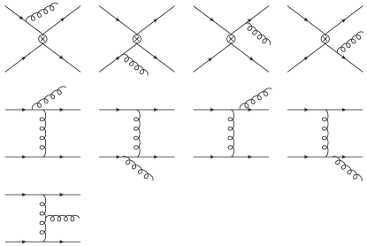
Figure 2: Real emission diagrams for both the SM QCD and NP contributions to $qq^{\prime}\to qq^{\prime}$ at the NLO.

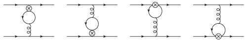
Figure 3: Additional penguin-like loop diagrams contributed to $qq^{\prime}\to qq^{\prime}$ at the NLO.

For the new physics contributions, beside from the loop diagrams in Fig. 1, there are some additional penguin-like loop diagrams as shown in Fig. 3. They generate infrared finite terms with mixing among operators with different chiral structures. After renormalization, we obtain both infrared and ultraviolet finite amplitudes

$$i\mathcal{M}^{v}_{NP,1} = i(\mathcal{M}_{1}+\mathcal{M}_{3}){\alpha_{s}\over 4\pi}\Big{\{}\Big{[}-{4\over 3}(c_{1}-{c_{2}\over 2N})\big{(}\ln({\mu_{R}^{2}\over-t})$$

$$+{2\over 3}\big{)}-{2n_{f}\over 3}c_{2}\big{(}\ln({\mu_{R}^{2}\over-t})+{5\over 3}\big{)}\Big{]}\mathcal{C}_{2}\Big{\}}/\Lambda^{2},$$

$$i\mathcal{M}^{v}_{NP,2} = i\mathcal{M}^{v}_{NP,1}\{\mathcal{M}_{1}\rightarrow\mathcal{M}_{2},c_{1}\rightarrow c_{5},c_{2}\rightarrow c_{6}\},$$

$$i\mathcal{M}^{v}_{NP,3} = i(\mathcal{M}_{1}+\mathcal{M}_{2}+2\mathcal{M}_{3}){\alpha_{s}\over 4\pi}\Big{\{}\Big{[}-{n_{f}\over 3}c_{4}\big{(}\ln({\mu_{R}^{2}\over-t})$$ (9)

$$+{5\over 3}\big{)}\Big{]}\mathcal{C}_{2}\Big{\}}/\Lambda^{2},$$

which will contribute to the NLO results through interference with $i\mathcal{M}_{NP}^{tree}$ and $i\mathcal{M}_{SM}^{tree}$ in Eq. (3.1).

3.2 Renormalization group running of Wilson coefficients

If the new physics scale $\Lambda$ at which the Wilson coefficients are derived is much higher than the physics scale considered at colliders, there will be large logarithm terms associated with these two scales in fixed order calculations. We can improve the convergence of the perturbative calculation by summing the logarithm contributions using the renormalization group (RG) evolution of the Wilson coefficients. The RG equation is given by

$${d\ c_{i}(\mu_{R})\over d\ \ln\mu_{R}}=\gamma(g)_{ij}\ c_{j}(\mu_{R}),$$ (10)

with the one-loop anomalous dimension matrix derived from Eq. (3),

$$\gamma(g)=-{\alpha_{s}\over 2\pi}\left(\begin{array}[]{cccccc}0&-{3C_{F}\over N}&0&0&0&0\\ -{22\over 3}&{20\over 3N}-{2\over 3}n_{f}&0&-{n_{f}\over 3}&0&0\\ 0&0&0&{3C_{F}\over N}&0&0\\ -{4\over 3}&{2\over 3N}-{2\over 3}n_{f}&6&6C_{F}-{3\over N}-{2\over 3}n_{f}&-{4\over 3}&{2\over 3N}-{2\over 3}n_{f}\\ 0&0&0&0&0&-{3C_{F}\over N}\\ 0&0&0&-{n_{f}\over 3}&-{22\over 3}&{20\over 3N}-{2\over 3}n_{f}\end{array}\right).$$ (11)

The RG improved NLO cross sections are defined as

$$\sigma_{NLO,RG}=\sigma_{NLO}+(\sigma_{RG}-\sigma_{RG}|_{NLO}),$$ (12)

where $\sigma_{RG}$ is the LO cross section calculated with RG improved Wilson coefficients and $\sigma_{RG}|_{NLO}$ is the expansion of $\sigma_{RG}$ up to NLO in QCD, which has already been included in $\sigma_{NLO}$. If only $c_{1}$ or $c_{2}$ is non-zero at the NP scale $\Lambda$, then the numerical solution of the RG equation that sums the LO logarithms are

$$c_{i}(\mu_{R})=c_{1}(\Lambda)X_{ij}r^{\gamma_{j}},\quad{\rm or}\quad c_{i}(\mu_{R})=c_{2}(\Lambda)Y_{ij}r^{\gamma_{j}},$$ (13)

where $r=\alpha_{s}(\mu_{R})/\alpha_{s}(\Lambda)$. The eigenvalues of the one-loop anomalous dimension matrix $\gamma$, after being divided by the overall factor $-{\alpha_{s}\over 2\pi}$ and $\beta_{0}$, are

$$\gamma_{i}=(-0.630,\,0.843,\,-0.487,\,0.342,\,0.275,\,-0.155),$$ (14)

where $\beta_{0}=(11N-2n_{f})/3$. Furthermore,

$$X_{ij} = \left(\begin{array}[]{cccccc}0.127&0.012&0.206&0.294&0.292&0.068\\ 0.462&-0.060&0.577&-0.577&-0.462&0.060\\ -0.130&0.045&0&0&-0.248&0.332\\ 0.470&0.218&0&0&-0.392&-0.296\\ 0.127&0.012&-0.206&-0.294&0.292&0.068\\ 0.462&-0.060&-0.577&0.577&-0.462&0.060\\ \end{array}\right),$$ (21)

$$Y_{ij} = \left(\begin{array}[]{cccccc}0.077&-0.018&0.105&-0.105&-0.076&0.016\\ 0.279&0.087&0.294&0.206&0.119&0.014\\ -0.078&-0.065&0&0&0.064&0.079\\ 0.284&-0.315&0&0&0.101&-0.071\\ 0.077&-0.018&-0.105&0.105&-0.076&0.016\\ 0.279&0.087&-0.294&-0.206&0.119&0.014\\ \end{array}\right).$$ (28)

In Fig.  4 we compare fixed order (NLO) and RG running of the Wilson coefficients $c_{1}$, $c_{2}$ and $c_{4}$ for $\Lambda=30\,{\rm TeV}$ assuming only $c_{1}$ (left panel) or $c_{2}$ (right panel) is non-zero at the NP scale $\Lambda$, with the renormalization scale ranges between $1\,{\rm TeV}$ and $30\,{\rm TeV}$. The running of the Wilson coefficients at the NLO can be obtained from the expansion of RG running in Eq. (13).

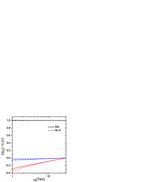
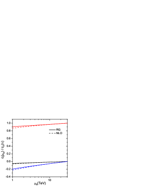
Figure 4: NLO and RG improved running of the Wilson coefficients. Curves from top to bottom correspond to $c_{1}$ (black), $c_{4}$ (blue) and $c_{2}$ (red) for the left panel, and $c_{2}$ (red), $c_{1}$ (black) and $c_{4}$ (blue) for the right panel.

4 Applications to quark compositeness search at the LHC

In this section we apply our NLO QCD results to the quark compositeness search at the LHC ($\sqrt{s}=7\,{\rm TeV}$) through dijet angular distribution measurement. For the numerical results here we assume only $c_{1}(\Lambda)$ and $c_{2}(\Lambda)$ to be non-zero, and parameterize them as $c_{1(2)}(\Lambda)=4\pi\lambda_{1(2)}$. Following conventions used in experimental analysis, for color-singlet case we have $|\lambda_{1(2)}|=1(0)$, while for color-octet case we have $|\lambda_{1(2)}|=0(1)$. We use the anti-$k_{t}$ jet algorithm Cacciari:2008gp with energy recombination scheme Bayatian:2006zz and the distance parameter $D=0.5$. To be considered as one of the two leading jets, a jet is required to satisfy the rapidity cut $|y|<3$. Moreover, we apply additional constraints on jet rapidity as below

$$|y_{b}|=|y_{1}+y_{2}|/2<1.11,\,\,\chi=\exp{(|y_{1}-y_{2}|)}<16,$$ (29)

to be consistent with the CMS measurement Khachatryan:2011as . $\chi$ is chosen as the dijet angular observable since after the Jacobian transformation the t-channel dominant SM QCD dijet production is almost flat on $\chi$. For massless jets, the invariant mass of dijet can be expressed as

$$m_{jj}=\sqrt{p_{T1}p_{T2}}\sqrt{\chi+1/\chi-2\cos(\Delta\phi)},$$ (30)

where $\Delta\phi$ is the azimuthal angle between the two jets. Considering the current experimental limits on the compositeness scale as well as the large SM QCD dijet background, NP contributions can only provide observable effects on the angular distribution in a very high dijet invariant mass region. Thus, below we will consider an invariant mass region between $[2\,{\rm TeV}$ and $3\,{\rm TeV}]$, and the part of theory parameter space with $\Lambda$ greater than $5\,{\rm TeV}$, for simplicity. In our numerical calculations, we use CTEQ6.6 parton distribution functions Nadolsky:2008zw and the corresponding running QCD coupling constant. Renormalization and factorization scales are set to be the average transverse momentum of the two leading jets, unless otherwise specified.

4.1 LO results and analysis

The LO total cross sections for dijet production induced by contact interactions consists of interference contributions with SM QCD amplitudes (denoted as $\sigma_{INT}$), as well as the NP squared contributions (denoted as $\sigma_{SQ}$). Assuming that only $c_{1}$ and $c_{2}$ are non-zero, the additional LO contribution

$$\sigma_{{\rm LO}} = \sigma_{INT}+\sigma_{SQ}$$

$$= (\lambda_{1}b_{{\rm L},1}+\lambda_{2}b_{{\rm L},2})/\Lambda^{2}+(\lambda_{1}^{2}b_{{\rm L},11}+\lambda_{2}^{2}b_{{\rm L},22}+\lambda_{1}\lambda_{2}b_{{\rm L},12})/\Lambda^{4},$$

where $b_{{\rm L},i(ij)}$ are independent of NP scale $\Lambda$ and $c_{i}=4\pi\lambda_{i}$. Instead of calculating the differential cross sections with respect to $\chi$, we choose two representative bins to investigate the influence of NP contributions to the dijet angular distribution, which are $\chi=[1,6]$ (bin 1) and $\chi=[6,11]$ (bin 2). The numerical results of $b_{{\rm L},i(ij)}$ are shown in Table 1. It can be seen that absolute values of $b$ for bin 1 are much larger than those for bin 2, which means the NP contributions could change the shape of $\chi$ distribution significantly since the SM QCD contributions are almost flat in $\chi$ distribution. It is also indicated in Table 1 that, even for a scale of $\Lambda$ as large as $5\,{\rm TeV}$, the NP squared terms can still be comparable to or even larger than the interference terms, especially for bin 1 of color-singlet case. Thus, the cross sections are not monotonous decreasing as $\Lambda$ increases, and zero point occurs for certain $\Lambda$ value with destructive interference. For simplicity, we will focus on the parameter region where the NP squared terms are relatively small, i.e., $\sigma_{SQ}/\sigma_{INT}<1$. Fig. 5 shows the absolute ratios of the NP contributions from the squared terms to the ones from the interference as functions of $\Lambda$, where for the color-singlet (octet) case we set $|\lambda_{1}|=1\,(0)$ and $|\lambda_{2}|=0\,(1)$ following the standard convention as mentioned before. Using the above condition, constraints on $\Lambda$ would be $\gtrsim 8\,{\rm TeV}$ for the color-singlet case and $\gtrsim 4\,{\rm TeV}$ for the color-octet case, which will be applied hereafter to our analysis.

[fb$\cdot$$(5\,{\rm TeV})^{2(4)}$]	$b_{{\rm L},1}$	$b_{{\rm L},2}$	$b_{{\rm L},11}$	$b_{{\rm L},22}$	$b_{{\rm L},12}$
bin 1	-258	-179	614	93.4	259
bin 2	-99.1	-70.4	113	17.2	46.8

Table 1: LO coefficients of NP contributions.

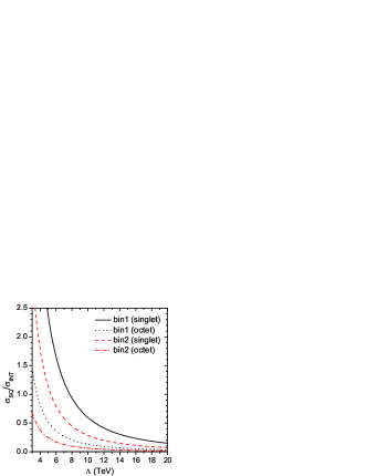
Figure 5: Ratios of NP squared contributions ($\sigma_{SQ}$) to SM and NP interference contributions ($\sigma_{INT}$) at the LO.

4.2 NLO results and analysis

At NLO, the total cross sections for dijet production induced by the contact interactions can be expressed as

$$\sigma_{{\rm NLO}} = \big{(}\lambda_{1}(b_{{\rm N},1}+a_{1}r)+\lambda_{2}(b_{{\rm N},2}+a_{2}r)\big{)}/\Lambda^{2}+\big{(}\lambda_{1}^{2}(b_{{\rm N},11}+a_{11}r)$$

$$+\lambda_{2}^{2}(b_{{\rm N},22}+a_{22}r)+\lambda_{1}\lambda_{2}(b_{{\rm N},12}+a_{12}r)\big{)}/\Lambda^{4},$$

where $b_{{\rm N},i(ij)}$ and $a_{i(ij)}$ are independent of the NP scale $\Lambda$, and $r=\ln(\Lambda/p_{0})$. We choose the reference scale

$$p_{0}=\langle{m}_{jj}\rangle/\sqrt{\langle\chi\rangle+1/\langle\chi\rangle+2},$$ (33)

where $\langle x\rangle$ denotes taking the average value of $x$ in the given bin of kinematic variables. Hence, $p_{0}$ is $1.04\,(0.77)\,{\rm TeV}$ for bin 1 (2).

The contributions proportional to $r$ represent running effects of the Wilson coefficients at NLO. Choosing same bins as in the LO analysis, we get the results for $b_{{\rm N},i(ij)}$ and $a_{i(ij)}$ listed in Table 2. Based on results from Tables 1 and 2, we plot the NLO K-factors as functions of the compositeness scale in Fig. 6 for both cases with destructive and constructive interferences. The shadow regions indicate parameter spaces where contributions from the NP squared terms are larger than the ones from the interference terms. K-factors are unstable there for destructive interference case due to large cancelations of cross sections between NP squared contributions and interference ones. Beyond the shadow regions, the NLO QCD corrections reduce the absolute values of the NP contributions to the cross sections significantly for all the parameter cases. These are mainly due to the large constant terms and also the large logarithms of $\Lambda$ from the virtual corrections, cf. Eqs. (3.4) and (3.5) in Sec. 3.1, especially in the large $\chi$ region. From Fig. 6 we can see that the K-factors deviate significantly from 1 especially for bin 2. Thus one may doubt the reliability of the NLO results, i.e., the convergency of the perturbation series. Indeed, the small K-factors are mainly due to the LO results used here. In order to compare with the LO theoretical results used by the experimentalist, by default we use fixed LO Wilson coefficients in the LO cross sections here and below. If we use the NLO running Wilson coefficients in the LO calculations instead, same as in the NLO calculations, then the K-factors will increase due to the suppression of the LO cross sections. Also the K-factors depend on the QCD scale choices, especially for large $\chi$ region. If we set the central scale to $p_{T,max}\exp(0.15|y_{1}-y_{2}|)$ as in the ATLAS dijet study Aad:2011fc , where $p_{T,max}$ is the transverse momentum of the hardest jet, then the K-factors will further increase. In Fig. 7 we show the K-factors calculated using this alternative definition of the LO cross sections in the perturbation series and choice of the scale. We can see that the NLO results are well behaved with reasonable K-factors that are relatively larger and stable as compared to the ones in Fig. 6.

[fb$\cdot$$(5\,{\rm TeV})^{2(4)}$]	$b_{{\rm N},1}$($a_{1}$)	$b_{{\rm N},2}$ ($a_{2}$)	$b_{{\rm N},11}$($a_{11}$)	$b_{{\rm N},22}$($a_{22}$)	$b_{{\rm N},12}$($a_{12}$)
bin 1	-232(20)	-159(19)	506(-26)	74.3(-12)	172(-51)
bin 2	-68.3(8.7)	-44.1(9.2)	89.2(-4.9)	13.0(-2.3)	33.1(-9.8)

Table 2: NLO coefficients of NP contributions.

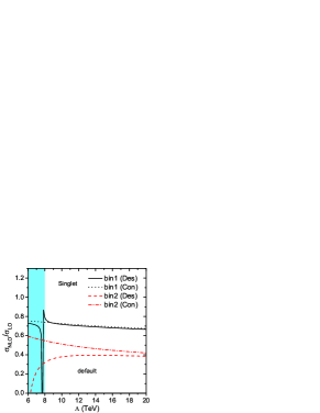
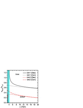
Figure 6: NLO K-factors, as functions of $\Lambda$, using the default definition of the LO cross sections and choice of scale.

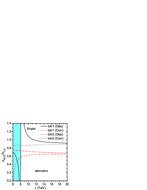
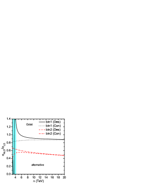
Figure 7: NLO K-factors, as functions of $\Lambda$, using the alternative definition of the LO cross sections and choice of scale.

In Fig. 8 we show NP contributions to the total cross sections of bin 1 with scale uncertainties to further investigate the improvement on scale dependence of the NLO results. The uncertainties are calculated by varying the factorization and renormalization scales, separately, for $\mu=\langle p_{T}\rangle/2$, $\mu=\langle p_{T}\rangle$, and $\mu=2\langle p_{T}\rangle$, where $\langle p_{T}\rangle$ is the average $p_{T}$ of the two leading jets. Generally, we can see a reduction of the scale uncertainties for the NLO results.

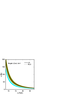
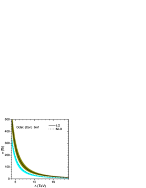
Figure 8: LO and NLO total cross sections, including scale uncertainties, as functions of $\Lambda$.

4.3 RG improved NLO results

As already mentioned in the analytical results, when the compositeness scale is much higher than the typical energy scale of experiments, we can sum over large logarithms of $\Lambda$, induced from higher order corrections, to improve the convergency of perturbative expansion. This leads to the RG improved NLO cross sections $\sigma_{\rm RG,NLO}$. It can deviate largely from the NLO cross sections in the large $\chi$ region where the jet $p_{T}$ is relatively small so that the running effects of Wilson coefficients are important. In Fig. 9, We show the ratios $\sigma_{\rm RG,NLO}/\sigma_{\rm LO}$ and $\sigma_{\rm RG,NLO}/\sigma_{\rm NLO}$ as a function of $\Lambda$. In general, the higher order corrections can increase the NLO total cross sections for both color singlet and octet cases, and the amount depends on the kinematic region considered. For example, for the bin 1 of color singlet case, the increase in $\sigma_{\rm RG,NLO}$ is about 3% and 10% of $\sigma_{\rm NLO}$ for $\Lambda=8\ {\rm TeV}$ and $30\ {\rm TeV}$, respectively. Moreover, the resumed contributions stabilize the K-factors of the total cross sections as compared to the NLO results for high $\Lambda$ values, which are around 0.7 and 0.5 for the bin 1 and the bin 2 of the color singlet case, respectively.

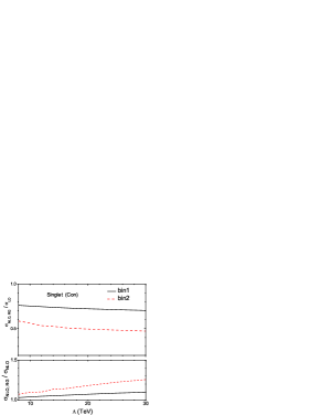
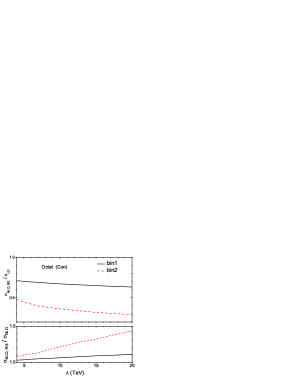
Figure 9: K-factors of the RGE improved NLO cross sections, as functions of $\Lambda$.

4.4 Exclusion limits of quark compositeness scale at the LHC

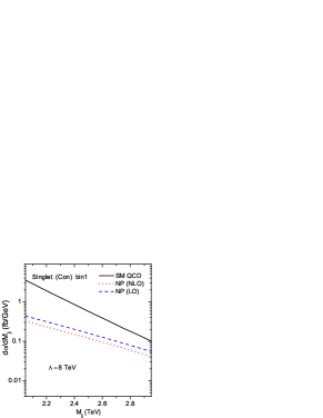
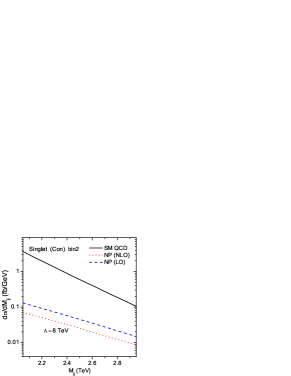
Figure 10: Dijet invariant mass distributions from the pure SM QCD contribution at NLO and the NP induced ones at both LO and NLO.

In order to directly compare our predictions to the experimental measurements, we need to combine them with the pure SM QCD contribution calculated at the NLO. We use a modified version of the EKS code Ellis:1992en to calculate the SM QCD dijet production at the NLO. We only consider the case of color-singlet with constructive interference in this section, and we do not include the RG improved corrections here since they are small for the considered $\Lambda$ values. In Fig. 10, we show comparisons of differential cross section from NP and pure SM contributions with invariant mass ranges from 2 to 3 $\rm TeV$ for the color-singlet case with constructive interference and $\Lambda=8\,{\rm TeV}$. As already mentioned before, the pure SM contributions in the two bins are almost the same, while the NP contributions are greatly different. To derive the expected exclusion limits of the compositeness scale, we further divide the invariant mass region $[2\,{\rm TeV},\,3\,{\rm TeV}]$ into 10 mass bins with equal width, and define the measure in each mass bin, $F_{\chi}(M_{jj})=\sigma_{\rm bin1}(M_{jj})/\sigma_{\rm bin2}(M_{jj})$. In Fig. 11, we plot theoretical predictions for $F_{\chi}(M_{jj})$ in different mass bins, where the (gray) solid vertical line represents the pseudo data expected by pure SM QCD contributions. The errors of the pseudo data include both the estimated statistical and systematical errors. The former is estimated by assuming Gaussian statistics with one standard deviation. Here, we assume a large data set with $\mathcal{L}=5\,{fb^{-1}}$ to calculate the statistical errors. We note that most of the experimental systematic uncertainties cancel in the ratio $F_{\chi}(M_{jj})$. For simplicity, we estimate an overall experimental systematic uncertainty of 3%, arising from the jet energy calibration and jet $p_{T}$ resolution for all the mass bins Khachatryan:2011as . The (colored) dashed and solid horizonal lines represent the SM QCD contributions plus NP contributions at LO and NLO, respectively. Fig. 11 shows that the NLO QCD corrections reduce the NP contributions to $F_{\chi}(M_{jj})$.

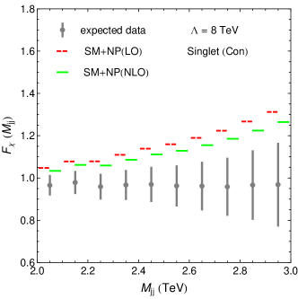
Figure 11: $F_{\chi}(M_{jj})$ for pseudo data estimated by pure SM QCD contribution, and for SM plus NP contributions at the LO and NLO, respectively.

On the other hand, the theoretical predictions also have uncertainties due to parton distribution functions, non-perturbative corrections, and most importantly the unknown higher order QCD corrections. The first two are found to be small according to the analysis in Ref Khachatryan:2011as . The conventional way to estimate the uncertainty from unknown higher order corrections is to examine its scale variations, i.e, to calculate the spread of the cross section over a set of scale choices. In Fig. 12(a), we show scale variations of the cross sections in different bins for SM plus NLO NP contributions, the spread are calculated by varying the factorization and renormalization scales independently for $\mu=\langle p_{T}\rangle/2$, $\mu=\langle p_{T}\rangle$, and $\mu=2\langle p_{T}\rangle$. For $F_{\chi}(M_{jj})=\sigma_{\rm bin1}(M_{jj})/\sigma_{\rm bin2}(M_{jj})$, we can independently vary the scales in both the numerator and denominator factors. Since there may be some correlations between these two parts in the missing higher order corrections, it will lead to an overestimation of the uncertainties. Here, we vary the scale simultaneously for cross sections in bin 1 and bin 2, and take half of the total scale variation of $F_{\chi}(M_{jj})$ as the estimated theoretical error. The corresponding theoretical errors of $F_{\chi}(M_{jj})$ for SM plus NLO NP contributions are shown in Fig. 12(b), which are around 4-7% in different invariant mass bins.

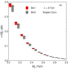
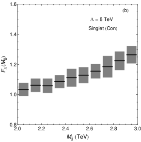
Figure 12: (a) Total cross sections in bin 1 and bin 2 with scale variations; (b) predictions of $F_{\chi}(M_{jj})$ with theoretical errors included. Both of them are for SM plus NLO NP contributions.

We perform a simple log-likelihood $\chi^{2}$ test for the hypothesis of NP with

$$\chi^{2}=\sum_{i=1,\,10}\frac{(F_{\chi}^{SM+NP}(i)-F_{\chi}^{SM}(i))^{2}}{\Delta_{exp}^{2}(i)+\Delta_{th}^{2}(i)},$$ (34)

where $F_{\chi}^{SM}(i)$ represents the pure SM contribution of $F_{\chi}(M_{jj})$ in the $i$th mass bin, which we assume to be the expected data, and $F_{\chi}^{SM+NP}(i)$ is the theory prediction given by SM plus NP contributions. $\Delta_{exp,\,th}$ represents the corresponding experimental errors and theoretical errors of $F_{\chi}^{SM+NP}(i)$, and we do not consider possible correlations of errors in different mass bins. The $\chi^{2}/N_{d.o.f}$ with $N_{d.o.f}=10$ are shown in Fig. 13 as functions of the compositeness scale $\Lambda$ for 3 cases, i.e, SM plus LO or NLO NP contributions without including the theoretical uncertainty, and SM plus NLO NP contributions with theoretical uncertainty included. Exclusion limits (95% C.L.) of $\Lambda$ can be read directly from Fig. 13 as intersections of the curves with the horizontal line. We can see that the theoretical uncertainty has a large effect on the exclusion limit since they are comparable with the experimental errors. With more data collected at the LHC, the statistical error will further decrease, then theoretical uncertainty will play a much more important role in the measurement.

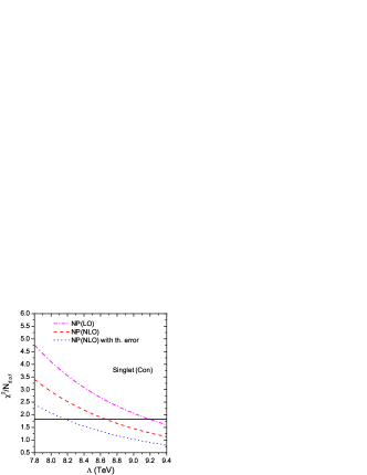
Figure 13: $\chi^{2}/N_{d.o.f}$ as functions of the compositeness scale $\Lambda$. Intersections of the curves with the horizontal line show the exclusion limits at the 95% C.L..

5 Conclusion

In conclusion, we have calculated the exact NLO QCD corrections to dijet production at the LHC, induced by quark contact interactions with different color and chiral structures from new physics. By applying our results to quark compositeness search at the LHC, we show that the NLO QCD corrections can lower the NP cross sections by several tens percent, depending on the choice of the theory parameters and the kinematic regions considered. Moreover, the NLO QCD corrections reduce the dependence of the cross sections on factorization and renormalization scales. We also calculate the renormalization group improved NLO cross sections by summing over the large logarithms induced from the running of Wilson coefficients, which are found to stabilize the K-factors at large quark compositeness scales. We further investigate the NLO QCD effects on the corresponding experimental observables and study the exclusion limits of the quark compositeness scale.

Appendix

In this appendix we briefly introduce our numerical code CIDIJET2.3, developed for the NLO QCD calculation of the dijet production induced by quark contact interaction.

Basically, this code is calculating the double differential cross sections in terms of the dijet invariant mass $M_{jj}$ and the angle parameter $\chi$. There are two calculation modes in this code. The first one is to numerically evaluate the fixed order double differential cross sections, in a kinematic bin specified by its range of $M_{jj}$ and $\chi$, for various values of $\Lambda$ and $c_{i}$ (or $\lambda_{i}$). For $c_{i}=4\pi\lambda_{i}$, the fixed order (LO or NLO) cross section can be written as

$$\sigma_{bin} = \sum_{i=1}^{6}(\lambda_{i}(b_{i}+a_{i}r))/\Lambda^{2}+\sum_{i=1}^{6}(\lambda_{i}^{2}(b_{ii}+a_{ii}r))/\Lambda^{4}$$ (35)

$$+\sum_{i=1,3,5}(\lambda_{i}\lambda_{i+1}(b_{ii+1}+a_{ii+1}r))/\Lambda^{4}$$

$$+\sum_{i=1,2,5,6}(\lambda_{i}\lambda_{4}(b_{i4}+a_{i4}r))/\Lambda^{4}.$$

with $r=\ln(\Lambda/p_{0})$, and $p_{0}$ is defined as in Eq. (33). The code can calculate all the above coefficients ($a$’s and $b$’s) directly, thus users do not need to repeat the calculations for different $\Lambda$ and $\lambda_{i}$ values. Since QCD interaction preserves parity conservation, we should have $b(a)_{1,2}=b(a)_{5,6}$, $b(a)_{11,22,12}=b(a)_{55,66,56}$, and $b(a)_{14,24}=b(a)_{54,64}$. The code has two dynamic QCD scale choices, which is average $p_{T}$ of two leading jets used by the CMS collaboration and $p_{T,max}\exp(0.15|y_{1}-y_{2}|)$ used by the ATLAS collaboration, and provides inputs of pre-factors for both renormalization and factorization scale to study the scale variations. Another mode is for the calculation of higher order corrections in addition to the NLO cross sections, which arise from the renormalization group running of the Wilson coefficients, as discussed in section 3.2. They are only significant at very large $\Lambda$ values and need to be recalculated for different inputs of $\Lambda$ and $\lambda_{i}$. The CIDIJET2.3 code is publicly available by request.

- (1) S. Chatrchyan et al. [CMS Collaboration], Phys. Lett. B 704, 123 (2011) [arXiv:1107.4771 [hep-ex]].
- (2) V. Khachatryan et al. [CMS Collaboration], Phys. Rev. Lett. 106, 201804 (2011) [arXiv:1102.2020 [hep-ex]];
- (3) G. Aad et al. [ATLAS Collaboration], New J. Phys. 13, 053044 (2011) [arXiv:1103.3864 [hep-ex]].
- (4) S. Chatrchyan et al. [CMS Collaboration], arXiv:1202.5535 [hep-ex].
- (5) G. Aad et al. [Atlas Collaboration], Eur. Phys. J. C 71, 1512 (2011) [arXiv:1009.5908 [hep-ex]]; S. Chatrchyan et al. [CMS Collaboration Collaboration], Phys. Lett. B 700, 187 (2011) [arXiv:1104.1693 [hep-ex]]; S. Chatrchyan et al. [CMS Collaboration], Phys. Rev. Lett. 107, 132001 (2011) [arXiv:1106.0208 [hep-ex]].
- (6) E. Eichten, K. D. Lane and M. E. Peskin, Phys. Rev. Lett. 50, 811 (1983); E. Eichten, I. Hinchliffe, K. D. Lane and C. Quigg, Rev. Mod. Phys. 56, 579 (1984) [Addendum-ibid. 58, 1065 (1986)]; P. Chiappetta and M. Perrottet, Phys. Lett. B 253, 489 (1991); O. Domenech, A. Pomarol and J. Serra, arXiv:1201.6510 [hep-ph].
- (7) K. D. Lane, arXiv:hep-ph/9605257.
- (8) F. Abe et al. [CDF Collaboration], Phys. Rev. Lett. 77, 5336 (1996) [Erratum-ibid. 78, 4307 (1997)]; T. Aaltonen et al. [CDF Collaboration], Phys. Rev. D 79, 112002 (2009); V. M. Abazov et al. [D0 Collaboration], Phys. Rev. Lett. 103, 191803 (2009).
- (9) G. Aad et al. [ATLAS Collaboration], Phys. Lett. B 694, 327 (2011); V. Khachatryan et al. [CMS Collaboration], Phys. Rev. Lett. 105, 262001 (2010).
- (10) J. Gao, C. S. Li, J. Wang, H. X. Zhu and C. P. Yuan, Phys. Rev. Lett. 106, 142001 (2011) [arXiv:1101.4611 [hep-ph]].
- (11) P. Langacker, Rev. Mod. Phys. 81, 1199 (2008).
- (12) L. Randall and R. Sundrum, Phys. Rev. Lett. 83, 3370 (1999) .
- (13) G. Buchalla, A. J. Buras and M. E. Lautenbacher, Rev. Mod. Phys. 68, 1125 (1996).
- (14) R. K. Ellis and J. C. Sexton, Nucl. Phys. B 269, 445 (1986).
- (15) B. W. Harris and J. F. Owens, Phys. Rev. D 65, 094032 (2002).
- (16) S. Catani and M. H. Seymour, Nucl. Phys. B 485, 291 (1997) [Erratum-ibid. B 510, 503 (1998)].
- (17) M. Cacciari, G. P. Salam and G. Soyez, JHEP 0804, 063 (2008).
- (18) G. L. Bayatian et al. [CMS Collaboration], CERN-LHCC-2006-001.
- (19) P. M. Nadolsky et al., Phys. Rev. D 78, 013004 (2008).
- (20) G. Aad et al. [ATLAS Collaboration], arXiv:1112.6297 [hep-ex].
- (21) S. D. Ellis, Z. Kunszt and D. E. Soper, Phys. Rev. Lett. 69, 1496 (1992).