Perturbative formulae for relativistic interactions of effective particles

Abstract

The concept of effective particles as degrees of freedom in a relativistic quantum field theory is defined using a non-perturbative renormalization group procedure for Hamiltonians. However, every candidate for a basic physical theory appears to require an initial perturbative search for the set of interaction terms that may provide a basis with which the full effective theory Hamiltonian could be constructed in a series of successive approximations. This article describes the required perturbative expansion and illustrates it with a set of general 4th-order formulae.

IFT/12/01

1 Introduction

The construction of relativistic interactions of effective particles that is described in this article is designed for a quantum theory in which one can introduce a front form (FF) of Hamiltonian dynamics [1]. The construction draws on the previous work on similarity renormalization group (SRG) procedure for Hamiltonians [2], flow equation [3], and renormalization group procedure for effective particles (RGPEP) [4]. It is the latter that is used here.

The key limitation of the RGPEP in comparison to the general SRG procedure [2] is that in RGPEP one focuses on coefficients of operators in an operator basis built from products of creation and annihilation operators for effective particles rather than on the Hamiltonian matrix elements. The requirement that the effective dynamics is obtained by universally rotating the bare particle operators to corresponding effective ones imposes unitary constraints on the effective theory. These constraints are not necessarily satisfied when one defines an effective Hamiltonian by rotating its matrix in some basis. In the matrix, many operators may contribute to one and the same matrix element and a rotation of a matrix does not have to be equivalent to a rotation of particle operators. In the effective particle theory, the matrix rotations one considers result only from rotating particle operators. This simplification allows one to encode many matrix elements in a small number of operators. In practice, the simplification begins to manifest itself when one considers states with more particles than 2 or 3. For example, a two-body effective potential term involves a product of only four fields and a function, say $v$, of their four arguments, such as in Secs. II E and X C in [5]. In contrast, a matrix element of the same term between states of many particles involves many copies of the function $v$ with different arguments. In addition, since the field operators involve both creation and annihilation operators, even an operator built from just four field operators requires a large space of states to study its matrix elements and uncover its actual operator structure as a result.

Derivation of the perturbative formulae for relativistic interactions of effective particles starts from the non-perturbative RGPEP equation that has been mentioned before in [6] on the basis of [7]. The starting RGPEP equation resembles Wegner’s [3] (for reviews, see [8, 9]) in its double commutator structure. Somewhat different perturbative expansions could be obtained in the RGPEP starting from the non-perturbative equations that involve multiple commutators. Such equations are described in Appendix A.

The relativistic nature of effective interactions is achieved using RGPEP by respecting the 7 kinematical symmetries of the FF of Hamiltonian dynamics [1] and cluster properties [10] in quantum field theory. The starting non-perturbative equation of RGPEP is designed to preserve these features. They are also preserved in the perturbative expansion. The running cutoff parameter of RGPEP limits only changes of the invariant mass of interacting particles. These features are required, for example, in application to QCD where one desires to simultaneously explain the constituent quark model classification of hadrons [11] and their quite different picture in the parton model [12].

Section 2 provides a brief account of the RGPEP and Section 3 describes the perturbative solution up to the 4th order. Section 4 concludes the paper. Appendix A describes multi-commutator flow equations and Appendix B provides universal formulae for coefficients in the perturbative expansion of effective Hamiltonian interaction terms.

2 Non-perturbative RGPEP [7]

Consider a local field theory in which fields on a given hyper-plane in the Minkowski space-time are expanded into their Fourier components. The components have interpretation of creation or annihilation operators of the field quanta. These quanta are called the bare, or initial particles, and the operators that create or annihilate them are called bare particle operators. The bare particle operators are generically denoted by $q_{0}$. A one-bare-particle state is obtained by acting with a creation operator $q_{0}$ on the vacuum state $|0\rangle$. The bare particle operators are used to build a basis in the Fock-space by acting with products of creation operators $q_{0}$ on $|0\rangle$.

Hamiltonian densities of canonical quantum field theories are built from products of fields and their derivatives. A Hamiltonian obtained by integrating such a density over a space-time hyperplane is a combination of products of operators $q_{0}$ with coefficients $c_{0}$. If a product contains $n$ particle operators, the coefficient has $n$ arguments. Each of the arguments represents a complete set of quantum numbers carried by a corresponding particle. One sums or integrates over these arguments in the Hamiltonian terms.

RGPEP introduces effective particle operators

$$q_{s} = {\cal U}_{s}\,q_{0}\,{\cal U}_{s}^{\dagger}\,,$$ (1)

labeled by the parameter $s$ which plays the role of a renormalization group parameter. This means that $s$ labels a family of Hamiltonians that all correspond to one and the same theory but are expressed in terms of differently defined degrees of freedom. All kinematical quantum numbers of $q$ are the same on both sides of Eq. (1), i.e., irrespective of the value of $s$.

The parameter $s$ has dimension of length and ranges from 0 to any finite number of choice, including arbitrarily large numbers. The larger $s$ the harder calculation of the corresponding Hamiltonian. $s\rightarrow\infty$ corresponds to solving for the spectrum of a theory. This is exemplified in the elementary model discussed below. In complex theories, where there is little hope for obtaining analytic solutions and one has to use numerical methods, the parameter $s$ may hopefully be kept, on the one hand, sufficiently small to maintain an analytically controlled connection with the quantum field theory one starts from, and, on the other hand, sufficiently large to enable numerical calculations using computers.

Physically, $s$ has the interpretation of the characteristic size of the effective particles. The interpretation follows from the fact that effective interactions contain form factors that limit how far off energy shell the interactions can extend. The width of the form factors is determined by $1/s$. Consequently, $s=0$ corresponds to the concept of point-like, bare particles in the case of a local quantum field theory. The effective Hamiltonian that corresponds to scale $s$ is band-diagonal on the energy scale (more precisely, on the scale of invariant masses of particles involved in an interaction) and the band width is $\sim 1/s$. The principle of using the band-diagonal structure for the purpose of renormalization is formulated in [2].

Let the initial Hamiltonian including counterterms be ${\cal H}_{0}(q_{0})$. For dimensional and notational reasons, it is convenient to use the parameter $t=s^{4}$ and label Hamiltonians and other operators with $t$ rather than $s$ itself. The RGPEP demands that

$${\cal H}_{t}(q_{t}) = {\cal H}_{0}(q_{0})\,.$$ (2)

This means that one changes particle operators from $q_{0}$ to $q_{t}$ and at the same time the coefficients $c_{0}$ are changed to $c_{t}$ so that the Hamiltonian operator stays unchanged. Consequently, the wave functions of its eigenstates, in a Fock-space basis built using $q_{t}$, depend on $t$. This design serves the purpose of simultaneously explaining the canonical picture of Hamiltonian eigenstates as built from bare, point-like particles, and the constituent picture in terms of extended, effective particles. Such setup is desired for solving QCD and comparing solutions with experimental data.

2.1 Generator

By differentiating both sides of

$${\cal H}_{t}(a_{0}) = {\cal U}^{\dagger}_{t}\,{\cal H}_{0}(a_{0})\,{\cal U}_{t}\,,$$ (3)

with respect to $t$, which is denoted by a prime, one obtains

$${\cal H}^{\prime}_{t}(a_{0}) = [-{\cal U}_{t}^{\dagger}{\cal U}^{\prime}_{t},{\cal H}_{t}(a_{0})]\,.$$ (4)

The product

$${\cal G}_{t} = -{\cal U}_{t}^{\dagger}{\cal U}^{\prime}_{t}$$ (5)

is called a generator. The RGPEP generator is defined by the formula

$${\cal G}_{t} = [{\cal H}_{f},{\cal H}_{Pt}]\,,$$ (6)

whose right-hand side will be explained below. The definition allows for adding arbitrary multiples of ${\cal H}_{t}(a_{0})$ or other operators that commute with ${\cal H}_{t}(a_{0})$ but such additions to ${\cal G}_{t}$ are ignored as immaterial here.

Since ${\cal G}_{t}$ is defined as a commutator of two formally hermitian operators, it is formally anti-hermitian, and ${\cal U}_{t}$ is formally unitary. The word “formal” is used here because precise definitions require regularization (see the quoted literature).

In what follows below, if an operator is expressed in terms of the basis operators $q_{0}$, they are no longer indicated as its arguments. However, one should remember that the effective Hamiltonian is obtained by making the substitution, $H={\cal H}_{t}(q_{t})={\cal H}_{t}(q_{0}\rightarrow q_{t})$. In the notation for operators $q_{0}$ themselves, the subscript $0$ is also omitted, so that $q\equiv q_{0}$.

2.2 ${\cal H}_{f}$ in Eq. (6)

The Hamiltonian ${\cal H}_{f}$, called the free Hamiltonian, is the part of a full Hamiltonian at $t=s^{4}=0$ that has the form

$${\cal H}_{f} = \sum_{i}\,p_{i}^{-}\,q^{\dagger}_{i}q_{i}$$ (7)

and does not depend on the interactions. More precisely, ${\cal H}_{f}$ is defined as the part of ${\cal H}$ that one is left with when the coupling constants in the initial theory are set to 0 and only the terms that are bilinear in fields are kept. The sum extends over all particle species and their quantum numbers so that the sum also includes integration over particle momenta $p$. The minus component of a particle momentum, $p_{i}^{-}=p_{i}^{0}-p_{i}^{3}$, in Eq. (7),

$$p^{-}_{i} = {p_{i}^{\perp\,2}+m_{i}^{2}\over p_{i}^{+}}\,,$$ (8)

is the FF energy that corresponds to a free particle with the mass $m_{i}$ and kinematical momentum components $p_{i}^{+}$ and $p_{i}^{\perp}$. Typically, different species of particles have different masses.

2.3 ${\cal H}_{Pt}$ in Eq. (6)

The operator ${\cal H}_{Pt}$ is uniquely defined once the Hamiltonian ${\cal H}_{t}$ is specified. If the Hamiltonian ${\cal H}_{t}$ is of the form

$${\cal H}_{t} = \sum_{n=2}^{\infty}\,\sum_{i_{1},i_{2},...,i_{n}}\,c_{t}(i_{1},...,i_{n})\,\,q^{\dagger}_{i_{1}}\cdot\cdot\cdot q_{i_{n}}\,,$$ (9)

where the coefficients $c_{t}(i_{1},...,i_{n})$ are to be found using RGPEP, the operator ${\cal H}_{Pt}$ is defined by

$${\cal H}_{t} = \sum_{n=2}^{\infty}\,\sum_{i_{1},i_{2},...,i_{n}}\,c_{t}(i_{1},...,i_{n})\,\,\left({1\over 2}\sum_{k=1}^{n}p_{i_{k}}^{+}\right)^{2}\,\,q^{\dagger}_{i_{1}}\cdot\cdot\cdot q_{i_{n}}\,.$$ (10)

Thus, ${\cal H}_{Pt}$ differs from ${\cal H}_{t}$ by multiplication of its terms by the square of $+$-component of total momentum carried by the particles in a term. This kinematical momentum is specified by the operator content of a term irrespective of the value of RGPEP parameter $t=s^{4}$.

The definition of ${\cal H}_{Pt}$ secures that both sides of Eq. (4), which now reads

$${d\over dt}\,{\cal H}_{t} = \left[[{\cal H}_{f},{\cal H}_{Pt}],{\cal H}_{t}\right]\,,$$ (11)

behave in the same way with respect to operations of kinematical LF symmetries. This implies that the effective particle size parameter $s$ is invariant with respect to the FF kinematical subgroup of the Poincaré group.

2.4 Construction of counterterms

The RGPEP Eq. (11) predicts the coefficients $c_{t}$ of products of $q_{t}$ in ${\cal H}_{t}(q_{t})$ provided the initial condition for ${\cal H}_{0}(q_{0})$ is available. However, when the initial Hamiltonian involves divergences, such as the ones due to a dynamical coupling of infinitely many degrees of freedom over an infinite range of scales, it cannot be considered a good initial condition. One can cut the infinities off by regularization, limiting the space of states and/or limiting the range of scales involved in interaction. With the cutoffs, the solutions lead to effective Hamiltonians that involve huge numbers (or zeros) instead of meaningful terms. The huge numbers result from the ratios of cutoffs to physical parameters. Zeros result from inverses of the huge ratios.

The situation is understood here as the one in which the initial Hamiltonian may reflect a physically interesting structure that is relevant when one imposes so small cutoffs on the dynamics that the divergences are replaced by relatively small terms and these terms do not obscure the initial structure beyond recognition. The question is then how a good effective Hamiltonian should depend on the cutoffs so that its predictions do not. If the predictions did depend on the cutoffs, one could not treat the cutoff theory as equivalent to some fundamental one. By the word “fundamental” it is meant here that the range of validity of a “fundamental” theory is expected to be vastly greater than the range limited by adjustable cutoffs.

Following [13, 14] and [2], the RGPEP involves determination of additional terms, called counterterms, that need to be included in the initial Hamiltonian in order to render the effective theory which may correspond to the Hamiltonian initially suggested as valid. The construction of counterterms follows the rules of SRG procedure [2, 4, 7]. There is no explicit condition of widening of the band toward high energies (large invariant masses), but the narrowness of the Hamiltonian (see next section) enables one to search for counterterms on the basis of a condition that all matrix elements of a Hamiltonian corresponding to some finite size $s$ of effective particles between states of finite invariant masses, are independent of the initial cutoffs. This condition provides as many equations to solve as there are matrix elements to consider. The number of equations may be large enough to specify the structure of counterterms up to a limited set of unknown finite numbers or functions. These numbers or functions, called finite parts of counterterms, can be constrained by symmetries [15] and phenomenology.

In general, the only method for solving Eq. (11) is to use successive approximations. One hopes that a candidate number $n$ for a solution, ${\cal H}_{t}^{(n)}$, can be inserted on the right-hand side to render a new candidate ${\cal H}_{t}^{(n+1)}$ on the left-hand side, and ${\cal H}_{t}^{(n+1)}$ can be subsequently inserted on the right-hand side in place of ${\cal H}_{t}^{(n)}$ to render ${\cal H}_{t}^{(n+2)}$ on the left-hand side, and so on. More precisely, the hope is that a well-defined solution is approximated with increasing accuracy when $n$ increases. Of course, one has to study theories case-by-case in order to establish if the RGPEP sequence converges [16]. In principle, one may obtain not only solutions for ${\cal H}_{t}$ with limit cycles [17], instead of just fixed points, but also the solutions with chaotic behavior as functions of $t$ [18, 19].

The conceptual and computational difficulty is that in each step of constructing successive approximations one may have to modify the counterterms and the modification is not dictated by the iteration procedure alone. Namely, one has to inspect dependence of the small-invariant-mass matrix elements of ${\cal H}_{t}^{(n)}$ at large $t$ on regularization present in ${\cal H}_{t}^{(n)}$ at $t=0$ and attempt to counter this dependence by modifying the ${\cal H}_{t}^{(n)}$ at $t=0$. The modifications may amount to redefinitions of a finite number of coupling constants or functions of particle quantum numbers. However, when one confronts the issue of relativistic description of confinement, the question of convergence is not answered in any form yet and the mechanism by which effective Hamiltonians develop confining forces at finite $t$ is strictly speaking not known.

The attractive feature of the RGPEP equation is that it allows for splitting of the integration process into many small steps, accompanied with rescaling of invariant masses so that one always operates with dimensionless quantities $s{\cal M}$, where ${\cal M}$ is a free invariant mass of the interacting effective particles and $s$ is their size parameter. Each small step can be executed using variety of well-known mathematical methods as in the case of the original Wilsonian procedure [13, 14]. Thus, the RGPEP provides a new tool for studying universality in relativistic quantum field theories (see Appendix A in [7]). This feature is of interest because a well-defined effective QCD Hamiltonian may be sought using the RGPEP irrespective of many details in the initial Hamiltonian. Namely, it should be sufficient to start with any Hamiltonian in a suitable universality class.

Nevertheless, in order to begin the process of constructing solutions of the RGPEP equations as outlined above, one has to suggest the terms that should be included in ${\cal H}_{t}^{(1)}$ and can be expected to have significant coefficients in ${\cal H}_{t}^{(n)}$ with large $n$. Initially, the only available tool for gathering such information about important terms is perturbation theory. This article illustrates a general algorithm for generating perturbative formulae for ${\cal H}_{t}$. The illustration includes a set of perturbative formula up to 4th order, derived in Section 3.

2.5 Narrowness

Solving Eq. (11) by successive approximations involves restrictions on how many terms are kept in the Hamiltonian. Each of these terms is written as a product of quantum fields. A priori, a FF ${\cal H}_{t}$ contains infinitely many terms [5]. A good approximate operator solution must be little sensitive to the terms that are missing. Assuming that one can identify a set of dominant operators, the mechanism of narrowing the Hamiltonians through Eq. (11) can be seen using an equation that results from projecting Eq. (11) on a subspace of the Fock space.

Following Appendix C in Ref. [7], one can introduce a projector on a subspace of physical interest in the Fock space. Both the subspace and projector are denoted by $R$. The projection involves fixing total kinematical momentum of states and a cutoff on their total invariant mass so that the concept of a trace becomes well-defined. Let

$${\cal H} = R\,{\cal H}_{t}R\,.$$ (12)

The correspondingly projected RGPEP equation reads

$${\cal H}^{\prime} = \left[[{\cal H}_{f},{\cal H}_{P}],{\cal H}\right]\,.$$ (13)

The condition that the trace of ${\cal H}^{2}$ does not depend on $t$, implies for matrix elements ${\cal H}_{mn}=\langle m|{\cal H}|n\rangle$ in the basis built from eigenstates $|m\rangle$ of ${\cal H}_{f}$ with eigenvalues $P^{-}_{fm}$, that

$$\left(\sum_{mn}|{\cal H}_{Imn}|^{2}\right)^{\prime} = -\sum_{km}(P^{-}_{fk}-P^{-}_{fm})^{2}|{\cal H}_{Ikm}|^{2}2P_{mk}^{+2}\leq 0\,,$$ (14)

where $P^{+}_{mk}$ is the total $+$-momentum of the particles that are involved in the interaction. In terms of the invariant masses,

$$\left(\sum_{mn}|{\cal H}_{Imn}|^{2}\right)^{\prime} = -2\sum_{km}({\cal M}^{2}_{km}-{\cal M}^{2}_{mk})^{2}|{\cal H}_{Ikm}|^{2}\leq 0\,,$$ (15)

where ${\cal M}_{km}$ denotes an invariant mass of the particles in state labeled with $k$ that are transformed through the interaction ${\cal H}_{I}$ to particles in the state labeled by $m$. Change of order of subscripts results in an invariant mass of particles in a different state. Spectators do not contribute to the invariant masses. The calculations are explicitly invariant under 7 kinematical transformations of the FF of Hamiltonian dynamics.

Eq. (15) means that the sum of moduli squared of all matrix elements of the interaction Hamiltonian decreases as $t$ increases until all off-diagonal matrix elements of the interaction Hamiltonian between states with different free invariant masses vanish. Section 3 shows this feature in a perturbative expansion for ${\cal H}_{t}$ in powers of ${\cal H}_{It}$.

2.6 Transformation ${\cal U}_{t}$

Transformation ${\cal U}_{t}$ is a solution to

$${\cal U}_{t}^{\prime} = -{\cal U}_{t}\,\,[{\cal H}_{f},{\cal H}_{Pt}]\,.$$ (16)

The initial condition is ${\cal U}_{0}=1$. Successive approximations generate ${\cal U}_{t}$ from a solution for ${\cal H}_{t}$. The general solution is

$${\cal U}_{t} = T\exp{\left(-\int_{0}^{t}d\tau\,[{\cal H}_{f},{\cal H}_{P\tau}]\right)}\,,$$ (17)

where $T$ orders operators from left to right in the order from a smallest to a largest of their arguments $t$. Perturbative expansion of Eq. (17) provides a perturbative solution for ${\cal U}_{t}$. Knowing ${\cal U}_{t}$, one can calculate operators that create or annihilate effective particles of size $s$ using Eq. (1) with $t=s^{4}$.

3 Perturbative formulae

Solution of Eq. (11) for coefficients of products of effective particle operators in ${\cal H}_{t}$, is described in this Section using the notation that proved useful before, in which Eq. (11) takes the form

$${\cal H}_{t\,ab}^{\prime} = -ab^{2}\,{\cal H}_{It\,ab}+\sum_{x}(p_{ax}\,ax+p_{bx}\,bx)\,{\cal H}_{It\,ax}\,{\cal H}_{It\,xb}\,.$$ (18)

The letters $a$, $b$, and $x$, denote configurations of particles. A configuration is a collection of quantum numbers that label particle operators.

An example illustrating the concept of configuration is shown in Fig. 1. In Fig. 1, the configuration $a$ includes particle operator labels contained in the sets denoted by 1 and 2, the configuration $x$ includes particle operator labels contained in the sets denoted by 1, 5 and 4, and the configuration $b$ includes particle operator labels contained in the sets denoted by 3 and 4. A subscript such as $ax$ refers to a coefficient of the product of particle operators in a Hamiltonian term ${\cal H}_{I}$ that changes a configuration $x$ to a configuration $a$, etc. In Fig. 1, ${\cal H}_{It\,ax}$ would correspond to a term in ${\cal H}_{It}$ that involves a product of creation operators labeled with quantum numbers in set 2 and a product of annihilation operators with labels contained in sets 5 and 4. ${\cal H}_{It\,xb}$ would correspond to a term that involves a product of creation operators labeled with quantum numbers in sets 1 and 5 and a product of annihilation operators with labels contained in set 3. Symbol $ax$ as a term in the equation denotes a difference of invariant masses squared, $ax={\cal M}^{2}_{ax}-{\cal M}^{2}_{xa}$. ${\cal M}_{ax}$ denotes an invariant mass corresponding to only those particle operator labels in a configuration $a$ that emerge as a result of interaction from the configuration $x$. Thus, $ax=-xa$. For example, in Fig. 1, ${\cal M}_{ax}$ denotes the invariant mass corresponding to the particle operator labels in set 2 and ${\cal M}_{xa}$ denotes the invariant mass corresponding to the particle operator labels in sets 5 and 4. Spectators do not contribute to these invariant masses. Thus, in Fig. 1, ${\cal M}_{ax}$ and ${\cal M}_{xa}$ do not include particle operator labels from set 1, while ${\cal M}_{xb}$ and ${\cal M}_{bx}$ do not include particle operator labels from set 4. The invariant masses are evaluated using kinematical momenta and eigenvalues of ${\cal H}_{f}$. A symbol such as $p_{ax}$ denotes the sum of $+$ components of all momenta that appear in the labels of creation operators (or of all annihilation operators, which is the same due to the momentum conservation) in a product in the Hamiltonian term that changes the configuration $x$ to $a$, etc. In Fig. 1, $p_{ax}$ denotes the sum of $+$ components of momenta contained in set $2$, which is the same as the sum of $+$ components of momenta contained in sets 5 and 4 together, while $p_{xb}$ denotes the sum of $+$ components of momenta contained in sets 1 and 5, which is the same as the sum of $+$ components of momenta contained in set 3.

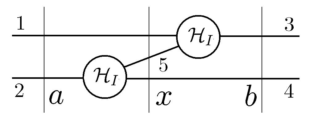
Figure 1: Example of the RGPEP operator calculus, see Eq. (18) and its description.

Key features of Eq. (18) are following. Since Eq. (18) only refers to quantum numbers that label particle operators, the Hamiltonian operators that solve Eq. (18) act in the entire Fock space. This is how the RGPEP procedure avoids the limitation to an a priori limited set of states that one is forced to work with using equations for Hamiltonian matrices. There are no disconnected terms in ${\cal H}_{t}$, since the second term in Eq. (18) results from a commutator. The commutator also implies that one keeps only the terms that result from commuting at least one annihilation operator with one creation operator in the product ${\cal H}_{It\,ax}\,{\cal H}_{It\,xb}$. Also, ${\cal H}_{t}$ does not explicitly depend on the eigenvalues of a full Hamiltonian. Such dependence is a serious limitation of all procedures that are in principle based on Gaussian elimination, or, in the path integral formulation, on integrating out the states outside a cut off in the space of states [14]. Namely, the larger an eigenvalue the worse accuracy of the procedure for integrating out the components above a cutoff.

The problem of integrating out states above a cutoff is circumvented in the RGPEP at the level of constructing counterterms and evaluating effective Hamiltonians. A finite remnant of this problem remains in an eigenvalue equation for ${\cal H}_{t}(q_{t})$, when one limits the space of states of effective particles that are included in a non-perturbative diagonalization using computers and when one fits finite parts of counterterms by comparison of theoretical results with experiment. This residual issue must be dealt with in the diagonalization procedure and typically should not cause problems because interactions do not grow with energy fast enough to generate any divergences. If they did cause divergences, a separate search for fixed points or other in principle possible behavior would have to be arranged (see Appendix B in [2]).

3.1 Form factors

Eq. (18) suggests that one writes

$${\cal H}_{t\,ab} = e^{-t\,ab^{2}}\,\,{\cal G}_{t\,ab}\,,$$ (19)

where

$$f_{t\,ab} = e^{-t\,ab^{2}}$$ (20)

is called a form factor. The width of the form factor as a function of the invariant mass change is $1/s$. Therefore, the parameter $s$ has the interpretation of a size of effective particles. It determines how far off shell an interaction can reach in terms of the invariant mass. The form factor secures narrowness of the effective Hamiltonian order-by-order in perturbation theory.

Eq. (18) implies that ${\cal G}_{t\,ab}$ satisfies the equation

$${\cal G}_{t\,ab}^{\prime} = \sum_{x}A_{t\,axb}\,{\cal G}_{t\,ax}\,{\cal G}_{t\,xb}\,,$$ (21)

where

$$A_{t\,axb} = (p_{\,ax}\,ax+p_{\,bx}\,bx)\,e^{-t(ax^{2}+xb^{2}-ab^{2})}\,.$$ (22)

Eq. (21) is solved below order-by-order in a perturbative expansion using powers of a single coupling constant $g$.

3.2 Expansion

When one expands

$${\cal G}_{t} = {\cal H}_{f}+g\,{\cal G}_{t1}+g^{2}\,{\cal G}_{t2}+g^{3}\,{\cal G}_{t3}+...\,,$$ (23)

the perturbative formulae for calculating ${\cal G}_{tn}$ is obtained in the form

$${\cal G}_{t\,n\,ab}^{\prime} = \sum_{k=1}^{n-1}\sum_{x}A_{t\,axb}\,{\cal G}_{t\,k\,ax}\,{\cal G}_{t\,n-k\,xb}\,.$$ (24)

It yields order-by-order the following differential equations

$${\cal G}^{\prime}_{t1\,ab} = 0\,,$$ (25)

$${\cal G}^{\prime}_{t2\,ab} = \sum_{x}A_{t\,axb}\,{\cal G}_{t1\,ax}\,{\cal G}_{t1\,xb}\,,$$ (26)

$${\cal G}^{\prime}_{t3\,ab} = \sum_{x}A_{t\,axb}\,\left({\cal G}_{t1\,ax}\,{\cal G}_{t2\,xb}+{\cal G}_{t2\,ax}\,{\cal G}_{t1\,xb}\right)\,,$$ (27)

$${\cal G}^{\prime}_{t4\,ab} = \sum_{x}A_{t\,axb}\,\left({\cal G}_{t1\,ax}\,{\cal G}_{t3\,xb}+{\cal G}_{t2\,ax}\,{\cal G}_{t2\,xb}+{\cal G}_{t3\,ax}\,{\cal G}_{t1\,xb}\right)\,.$$ (28)

The four terms indicate a generic pattern. This pattern is different from the patterns described in perturbative expansions studied using matrix models in Refs. [23] and [24]. The main reasons for the patterns to differ are the constancy of ${\cal H}_{f}$, which is of order 1, and the definition of ${\cal H}_{P}$ in Eq. (11), which leads to the factors of $+$-momentum of active particles in Eq. (22).

The same factors of $p^{+}$ appear in the procedure studied in Ref. [24], but there they are accompanied by appearance of the derivative of ${\cal G}^{\prime}$ on the right-hand side of the RGPEP equation for ${\cal H}^{\prime}$, in the generator. The derivatives in the generator cause additional difficulties in solving the RGPEP equation non-perturbatively. Here, the origin of factors of $p^{+}$ is in ${\cal H}_{Pt}$. The absence of derivatives in the generator remedies the additional difficulties encountered in Ref. [24].

General formulae for solutions of Eq. (24) are listed below order-by-order for all terms up to the 4th order, i.e., up to 2 or 3 loops in theories of the type $\phi^{3}$ or $\phi^{4}$, respectively, where the power of $\phi$ indicates how many field operators can be present in a term. This covers in principle all cases of interest in physics (except for gravity, because of the FF limitation to the Minkowski metric). For example, the expansion to 4th order is in principle sufficient to study interactions of constituent quarks in hadrons including the leading effects of self-interaction, gluon exchange, and running coupling constant. Such studies should clarify if the 4th order RGPEP is capable of generating information about the essentially non-canonical effective QCD interaction terms discussed in Ref. [5], or one must explore orders higher than 4 to see the new terms. Terms of higher orders can be generated as required according to the pattern visible in what follows.

3.3 Solutions, order-by-order

Appendix B describes details of solving Eqs. (25) to (28). This section lists the results, introducing the elements of notation developed in Appendix B.

3.3.1 1st-order solution

The first-order solution does not depend on $t$,

$${\cal G}_{t1\,ab} = {\cal G}_{01\,ab}\,.$$ (29)

The subscript 0 refers to $t=0$. Operators with subscript 0 are contained in the initial Hamiltonian. They provide the initial conditions.

The first-order initial condition includes a bare coupling constant, $g$, as a coefficient in front of a definite canonical operator. Counterterms of higher orders typically include the same operator. The net result of including counterterms is a change of value of $g$. The magnitude of change depends on the interaction terms included in and regularization method adopted for the initial canonical Hamiltonian.

3.3.2 2nd-order solution

The second-order solution reads

$${\cal G}_{t2\,ab} = {\cal G}_{02\,ab}+\sum_{x}B^{(123,0)}_{t\,axb}\,{\cal G}_{02\,axb}\,.$$ (30)

The initial condition ${\cal G}_{02\,ab}$ typically includes instantaneous interactions, such as a FF counterpart of the Coulomb interaction term in the standard form of dynamics, or instantaneous fermion terms that are unique to the FF of dynamics, due to constraints. The RGPEP may provide the higher-order terms that have similar structure but whose coefficients are not necessarily constrained according to the simple Heisenberg equations of motion that one might expect from the analogy with classical field equations [22]. For example, quantum interactions may lead to anomalies. The initial condition ${\cal G}_{02\,ab}$ also includes self-interaction counterterms.

The operator structure ${\cal G}_{02\,axb}$ is defined in Eq. (42). It results from action of first-order terms twice. The coefficient $B^{(123,0)}$ is defined in Eq. (48). The superscript convention is explained in Appendix B.1. It is well-known that the second-order terms reproduce standard second-order results for observables to the extent they are available in all theories relevant to physics.

3.3.3 3rd-order solution

The third-order solution reads

$${\cal G}_{t3\,ab} = {\cal G}_{03\,ab}+\sum_{x}B^{(123,0)}_{t\,axb}\,{\cal G}_{03\,axb}$$ (31)

$$+ \sum_{xy}\,\left[B^{(124,(234,0))}_{t\,axyb}+B^{(134,(123,0))}_{t\,axyb}\right]\,{\cal G}_{03\,axyb}\,.$$

The term ${\cal G}_{03\,ab}$ is an initial condition for an operator that does not appear in a canonical Hamiltonian. Namely, it is a third-order coupling constant counterterm. Operators ${\cal G}_{03\,axb}$ involve a product of two operators from the initial Hamiltonian: one of first order and another one of second order, see Eq. (43). The last operator, ${\cal G}_{03\,axyb}$, is a product of three first-order operators, see Eq. (44). The coefficients $B^{(124,(234,0))}_{t\,axyb}$ and $B^{(134,(123,0))}_{t\,axyb}$ are defined in Eqs. (49) and (50) in Appendix B.1.

The third-order solution of Eq. (31) slightly differs from the third-order formula previously studied using RGPEP in the cases of scalar theories in 6 dimensions [20] and in QCD in 4 dimensions [21]. Although the previous experience suggests that Eq. (31) leads to the same result concerning asymptotic freedom, the finite invariant-mass details of Eq. (31) are of special interest since they contribute to the fourth-order terms. The fourth-order terms required prohibitively complex equations in the previous applications of RGPEP. A relatively compact fourth-order solution is now made available in the next section.

3.3.4 4th-order solution

The fourth-order solution reads

$${\cal G}_{t4\,ab} = {\cal G}_{04\,ab}+\sum_{x}B^{(123,0)}_{t\,axb}\,{\cal G}_{04\,axb}$$ (32)

$$+ \sum_{xy}\left[B^{(124,(234,0))}_{t\,axyb}+B^{(134,(123,0))}_{t\,axyb}\right]\,{\cal G}_{04\,axyb}$$

$$+ \sum_{xyz}\left[B^{(125,(235,(345,0)))}_{t\,axyzb}+B^{(125,(245,(234,0)))}_{t\,axyzb}+B^{(145,(124,(234,0)))}_{t\,axyzb}\right.$$

$$+ \left.B^{(145,(134,(123,0)))}_{t\,axyzb}+B^{(135,(123,0),(345,0))}_{t\,axyzb}\right]\,{\cal G}_{04\,axyzb}\,.$$

The initial condition ${\cal G}_{04\,ab}$ is the fourth-order counterterm. It includes the self-interaction and coupling-constant counterterms that involve additional particles in an interaction. It also includes box-diagram counterterms, where they are needed. The operator ${\cal G}_{04\,axb}$ is defined in Eq. (45), the operator ${\cal G}_{04\,axyb}$ is defined in Eq. (46), and the operator ${\cal G}_{04\,axyzb}$ is defined in Eq.(47). The new coefficients in fourth order terms are defined in Eqs. (51) to (55).

The general fourth-order result opens a door to many specific studies. Perhaps one of the most instructive ones would be a calculation of $\Upsilon$ family masses and decay width, which is likely to shed some light on the dynamics of gluons in heavy quarkonia, cf. [25].

4 Conclusion

The perturbative RGPEP formulae of Section 3 allow one to study low-order divergences and effective interactions in specific theories with infinitesimal coupling constants and extreme cutoffs in their canonical Hamiltonians. They also provide a tool for testing the formal RGPEP claim of narrowness of effective theories described in Section 2. Such tests are essential because of anomalies, i.e., the new Hamiltonian terms that do not correspond to classical Lagrangians and instead result from imposing some regularization on a formal quantum theory. One potential source of anomalies that needs to be studied is a lower bound on $+$-momenta of particles in a Fourier analysis of a quantum field. Strictly speaking, such lower bound violates boost invariance of a formal theory.

Regarding systematic checks of existence of anomalies in the FF of Hamiltonian dynamics, there is currently no alternative known to the author to inspecting theories order-by-order using the RGPEP and finding out term-by-term if and how soon a specific regularization method in a given theory may generate anomalies in the weak-coupling expansion. Moreover, there is currently nothing known yet for certain about the anomalies generated in the FF of Hamiltonian dynamics using RGPEP.

The subject certainly deserves a study in view of the fact that the FF vacuum problem is differently formulated from the instant form vacuum problem. For example, if one imposes the above mentioned lower bound on $+$-momenta of particles in a Fourier analysis of quantum fields, the mathematical vacuum state, i.e., the state that is annihilated by bare annihilation operators, is an exact eigenstate of the full Hamiltonian with eigenvalue 0. If this state can play the role of the true ground state, the mechanisms of symmetry breaking and mass generation in effective theories may in principle turn out not to be associated with the vacuum expectation values of normal-ordered products of quantum fields but with some new terms in the Hamiltonians [5]. The perturbative RGPEP formulae for relativistic interactions of effective particles derived in Section 3.3 provide a new tool for studies of such hypotheses.

Most interestingly, however, the perturbative studies may help in identifying a finite set of operators that one can use to approximately solve the RGPEP Eq. (18) non-perturbatively, i.e., in terms of the coefficients in front of the identified operators. As functions of $t$, these coefficients would be expected to evolve from a set of constants and regulating functions at $t=0$ to a set of finite, non-trivial functions of particle quantum-numbers at some $t_{0}=s_{0}^{4}$, where $s_{0}$ denotes some size of the effective constituents that are most suitable as degrees of freedom for specific purposes of phenomenology.

Appendix A Multicommutator RGPEP

One can obtain narrow relativistic Hamiltonians using equations with an odd number of commutators. Namely, one can write

$${d\over dt}\,{\cal H}_{t} = \left[[{\cal H}_{f},[...{\cal H}_{f},[{\cal H}_{f},{\cal H}_{Pt}]...]],{\cal H}_{t}\right]\,,$$ (33)

including $2n-1$ operators ${\cal H}_{f}$ in a sequence of commutators with $n>1$ and $t=s^{4n}$. Correspondingly, one can define the operator ${\cal H}_{Pt}$ by writing

$${\cal H}_{t} = \sum_{n=2}^{\infty}\,\sum_{i_{1},i_{2},...,i_{n}}\,c_{t}(i_{1},...,i_{n})\,\,\left({1\over 2}\sum_{k=1}^{n}p_{i_{k}}^{+}\right)^{2n}\,\,q^{\dagger}_{i_{1}}\cdot\cdot\cdot q_{i_{n}}\,,$$ (34)

instead of Eq. (10). The resulting counterpart of Eq. (18) reads (cf. [7], footnote 43)

$${\cal H}_{t\,ab}^{\prime} = -ab^{2n}{\cal H}_{It\,ab}+\sum_{x}(p_{ax}ax^{2n-1}+p_{bx}bx^{2n-1})\,{\cal H}_{It\,ax}{\cal H}_{It\,xb}.$$ (35)

The narrowness is obtained for the matrices of projected Hamiltonians as in Section 2.5. However, instead of condition (15), one obtains a similar inequality with $({\cal M}^{2}_{km}-{\cal M}^{2}_{mk})^{2n}$ in place of $({\cal M}^{2}_{km}-{\cal M}^{2}_{mk})^{2}$. The perturbative expansion proceeds without any qualitative change, but the form factors in Section 3.1 are of the form

$$f_{t\,ab} = e^{-t\,ab^{2n}}\,.$$ (36)

Appendix B Calculation of the 4th-order terms

This Appendix contains a derivation of the fourth-order term described in Section 3.3. It also explains the pertinent notation. The calculation involves all terms of orders lower than 4. Using solutions given in Eqs. (29), (30), and (31), one obtains from Eq. (28) that

$${\cal G}^{\prime}_{t4\,ab} = \sum_{x}A_{t\,axb}\,\left({\cal G}_{01\,ax}\,{\cal G}_{03\,xb}+{\cal G}_{03\,ax}\,{\cal G}_{01\,xb}+{\cal G}_{02\,ax}\,{\cal G}_{02\,xb}\right)$$ (37)

$$+ \sum_{xy}A_{t\,axb}\,B^{(123,0)}_{t\,xyb}\,\left({\cal G}_{01\,ax}\,{\cal G}_{03\,xyb}+{\cal G}_{02\,ax}\,{\cal G}_{02\,xyb}\right)$$

$$+ \sum_{xy}A_{t\,ayb}\,B^{(123,0)}_{t\,axy}\,\left({\cal G}_{03\,axy}\,{\cal G}_{01\,yb}+{\cal G}_{02\,axy}\,{\cal G}_{02\,yb}\right)$$

$$+ \sum_{xyz}A_{t\,axb}\,\left[B^{(124,(234,0))}_{t\,xyzb}+B^{(134,(123,0))}_{t\,xyzb}\right]\,{\cal G}_{01\,ax}\,{\cal G}_{03\,xyzb}$$

$$+ \sum_{xyz}A_{t\,azb}\,\left[B^{(124,(234,0))}_{t\,axyz}+B^{(134,(123,0))}_{t\,axyz}\right]\,{\cal G}_{03\,axyz}\,{\cal G}_{01\,zb}$$

$$+ \sum_{xyz}A_{t\,ayb}\,B^{(123,0)}_{t\,axy}\,B^{(123,0)}_{t\,yzb}\,{\cal G}_{02\,axy}\,{\cal G}_{02\,yzb}\,,$$

where

$${\cal G}_{02\,axb} = {\cal G}_{01\,ax}\,{\cal G}_{01\,xb}\,,$$ (38)

$${\cal G}_{03\,axb} = {\cal G}_{01\,ax}\,{\cal G}_{02\,xb}+{\cal G}_{02\,ax}\,{\cal G}_{01\,xb}\,,$$ (39)

$${\cal G}_{03\,axyb} = {\cal G}_{01\,ax}\,{\cal G}_{01\,xy}\,{\cal G}_{01\,yb}\,.$$ (40)

Inserting these definitions and grouping coefficients in front of the same operators, one obtains the derivative of fourth-order terms in the form

$${\cal G}^{\prime}_{t4\,ab} = \sum_{x}A_{t\,axb}\,\left({\cal G}_{01\,ax}\,{\cal G}_{03\,xb}+{\cal G}_{03\,ax}\,{\cal G}_{01\,xb}+{\cal G}_{02\,ax}\,{\cal G}_{02\,xb}\right)$$ (41)

$$+ \sum_{xy}\left[A_{t\,axb}\,B^{(123,0)}_{t\,xyb}+A_{t\,ayb}\,B^{(123,0)}_{t\,axy}\right]$$

$$\times \left({\cal G}_{01\,ax}\,{\cal G}_{01\,xy}\,{\cal G}_{02\,yb}+{\cal G}_{01\,ax}\,{\cal G}_{02\,xy}\,{\cal G}_{01\,yb}+{\cal G}_{02\,ax}\,{\cal G}_{01\,xy}\,{\cal G}_{01\,yb}\right)$$

$$+ \sum_{xyz}\left(A_{t\,axb}\,\left[B^{(124,(234,0))}_{t\,xyzb}+B^{(134,(123,0))}_{t\,xyzb}\right]\right.$$

$$+ \left.A_{t\,azb}\,\left[B^{(124,(234,0))}_{t\,axyz}+B^{(134,(123,0))}_{t\,axyz}\right]+A_{t\,ayb}\,B^{(123,0)}_{t\,axy}\,B^{(123,0)}_{t\,yzb}\right)$$

$$\times {\cal G}_{01\,ax}\,{\cal G}_{01\,xy}\,{\cal G}_{01\,yz}\,{\cal G}_{01\,zb}\,.$$

The integration yields Eq. (32), which is written in Section 3.3.4 using the notation for operators and coefficients that is described below in Appendix B.1.

B.1 Summary of terms and coefficients

The operators that emerge up to the fourth order in Section 3.3 are

$${\cal G}_{02\,axb} = {\cal G}_{01\,ax}\,{\cal G}_{01\,xb}\,,$$ (42)

$${\cal G}_{03\,axb} = {\cal G}_{01\,ax}\,{\cal G}_{02\,xb}+{\cal G}_{02\,ax}\,{\cal G}_{01\,xb}\,,$$ (43)

$${\cal G}_{03\,axyb} = {\cal G}_{01\,ax}\,{\cal G}_{01\,xy}\,{\cal G}_{01\,yb}\,,$$ (44)

$${\cal G}_{04\,axb} = {\cal G}_{01\,ax}\,{\cal G}_{03\,xb}+{\cal G}_{02\,ax}\,{\cal G}_{02\,xb}+{\cal G}_{03\,ax}\,{\cal G}_{01\,xb}\,,$$ (45)

$${\cal G}_{04\,axyb} = {\cal G}_{01\,ax}\,{\cal G}_{01\,xy}\,{\cal G}_{02\,yb}+{\cal G}_{01\,ax}\,{\cal G}_{02\,xy}\,{\cal G}_{01\,yb}$$ (46)

$$+ {\cal G}_{02\,ax}\,{\cal G}_{01\,xy}\,{\cal G}_{01\,yb}\,,$$

$${\cal G}_{04\,axyzb} = {\cal G}_{01\,ax}\,{\cal G}_{01\,xy}\,{\cal G}_{01\,yz}\,{\cal G}_{01\,zb}\,.$$ (47)

The corresponding coefficients are

$$B^{(123,0)}_{t\,axb} = \int_{0}^{t}d\tau\,A_{\tau\,axb}\,,$$ (48)

$$B^{(124,(234,0))}_{t\,axyb} = \int_{0}^{t}d\tau\,A_{\tau\,axb}\,B^{(123,0)}_{\tau\,xyb}\,,$$ (49)

$$B^{(134,(123,0))}_{t\,axyb} = \int_{0}^{t}d\tau\,A_{\tau\,ayb}\,B^{(123,0)}_{\tau\,axy}\,,$$ (50)

$$B^{(125,(235,(345,0)))}_{t\,axyzb} = \int_{0}^{t}d\tau\,A_{\tau\,axb}\,B^{(124,(234,0))}_{\tau\,xyzb}\,,$$ (51)

$$B^{(125,(245,(234,0)))}_{t\,axyzb} = \int_{0}^{t}d\tau\,A_{\tau\,axb}\,B^{(134,(123,0))}_{\tau\,xyzb}\,,$$ (52)

$$B^{(145,(124,(234,0)))}_{t\,axyzb} = \int_{0}^{t}d\tau\,A_{\tau\,azb}\,B^{(124,(234,0))}_{\tau\,axyz}\,,$$ (53)

$$B^{(145,(134,(123,0)))}_{t\,axyzb} = \int_{0}^{t}d\tau\,A_{\tau\,azb}\,B^{(134,(123,0))}_{\tau\,axyz}\,,$$ (54)

$$B^{(135,(123,0),(345,0))}_{t\,axyzb} = \int_{0}^{t}d\tau\,A_{\tau\,ayb}\,B^{(123,0)}_{\tau\,axy}\,B^{(123,0)}_{\tau\,yzb}\,.$$ (55)

The function $A_{t\,axb}$ is defined in Eq. (22). The convention for superscripts in coefficients $B$ is designed to reflect the origin of corresponding terms. Every coefficient has a subscript in the form of a list of particle configurations. The configurations are numbered with natural numbers from left to right. The numbers in the superscripts, indicate which configuration appears as a label in a corresponding factor under the integral. The first three numbers in a superscript refer to subscripts of $A$ defined in Eq. (22) and the remaining numbers refer to the subscripts in coefficients that form other factors under the integrals, according to the pattern illustrated by Eqs. (48) to (55).

References

- [1] P. A. M. Dirac, Rev. Mod. Phys. 21, 392 (1949).
- [2] S. D. Głazek, K. G. Wilson, Phys Rev. D 48, 5863 (1993).
- [3] F. Wegner, Ann. Phys. (Leipzig) 3, 77 (1994).
- [4] S. D. Głazek, Acta Phys. Pol. B 29, 1979 (1998).
- [5] K. G. Wilson et al., Phys. Rev. D 49 6720 (1994).
- [6] S. D. Głazek, Few-Body Syst. DOI 10.1007/s00601-011-0282-1.
- [7] S. D. Głazek, Acta Phys. Pol. B 42, 1933 (2011), and refs. therein.
- [8] F. Wegner, J. Phys. A: Math. Gen. 39, 8221 (2006).
- [9] S. K. Kehrein, The Flow Equation Approach to Many-Particle Systems, (Springer, 2006).
- [10] S. Weinberg, Quantum Theory of Fields I (Cambridge University Press, 1995).
- [11] K. Nakamura et al., J. Phys. G 37, 075021 (2010).
- [12] R. P. Feynman, Phys. Rev. Lett. 23, 1415 (1969).
- [13] K. Wilson, Phys. Rev. 140, B 445 (1965).
- [14] K. G. Wilson, Phys. Rev. D 2, 1438 (1970).
- [15] R. J. Perry, K. G. Wilson, Nucl. Phys. B 403, 587 (1993).
- [16] K. G. Wilson, M. E. Fisher, Phys. Rev. Lett. 28, 240 (1972).
- [17] K. G. Wilson Phys. Rev. D 3, 1818 (1971).
- [18] S. D. Głazek, K. G. Wilson Phys. Rev. B 69, 094304 (2004).
- [19] S. D. Głazek Phys. Rev. D 75, 025005 (2007).
- [20] S. D. Głazek, Phys. Rev. D 60, 105030 (1999).
- [21] S. D. Głazek, Phys. Rev. D 63, 116006 (2001).
- [22] P. A. M. Dirac, Phys. Rev. 139, B 684 (1965).
- [23] S. D. Głazek, J. Młynik, Phys. Rev. D 67, 045001 (2003).
- [24] S. D. Głazek, J. Młynik, Acta Phys. Pol. B 35, 723 (2004).
- [25] S. D. Głazek, J. Młynik, Phys. Rev. D 74, 105015 (2006).