Charge Fractionalization in a Mesoscopic Ring

Abstract

We study the fractionalization of an electron tunneling into a strongly interacting electronic one-dimensional ring. As a complement to transport measurements in quantum wires connected to leads, we propose non-invasive measures involving the magnetic field profile around the ring to probe this fractionalization. In particular, we show that the magnetic-field squared produced by the electron and the power that it would induce in a detector exhibit anisotropic profiles that depend on the degree of fractionalization. We contrast true fractionalization with two other scenarios which could mimic it – quantum superposition and classical probabilistic electron insertion. We show that the proposed field-dependent measures and those of the persistent current can distinguish between these three scenarios.

A spectacular feature of strongly correlated low-dimensional electronic systems is that collective behavior renders the electron completely unstable, resulting in its fractionalization review . As a prime example, in a one-dimensional quantum wire, Tomonaga-Luttinger liquid (TLL) theory predicts that a momentum-resolved electron tunneling into the wire splinters into charges $(1\pm g)e/2$ moving in opposite directions, where $g$, the Luttinger parameter depends on the ratio of interactions and Fermi energy and is unity in the absence of interactions safi ; pham . Exciting developments in experimental capabilities have enabled the physical realization of such a situation steinberg . These studies inspire revisiting fractionalization in a new light and addressing a spectrum of theoretical and physical issues. For instance, can one distinguish true fractionalization from quantum mechanical probabilistic processes? Or even classical probabilities? Are there geometries which could eliminate one of the biggest banes in detecting fractionalization – the effect of leads safi ; stone ; pugnetti ; kim ; frequency ? What measurements in such geometries could pinpoint true fractionalization? In this Letter, we answer each of these questions in the context of the ring geometry illustrated in Fig. 1.

Here, an electron tunnels from a lead into a thin mesoscopic ring and, as with the quantum wire leurtheory , has a well-defined momentum profile. Strong interactions within the ring cause an electron associated, for instance, with clockwise Fermi-momentum to decompose into two components of charge $(1\pm g)e/2$ moving in clockwise (CW) and counter-clockwise (CCW) directions. Our study focuses on the magnetic field produced by such a situation and the signatures of fractionalization reflected in the spatial distribution of higher moments involving this field. Specifically, we propose measurements of the field squared, as for instance can be measured by a SQUID, and the power induced by the field in a pickup loop (see Fig. 1). These measurements have the advantage of purely entailing d.c. quantities as opposed to high frequency measurements and of constituting weak, i.e., non-invasive, read-outs when compared with those involving lead attachment.

Fractionalization emerges from the strongly correlated nature of the many-body wavefunction and is fundamentally different from quantum mechanical superpositions or classical probabilities involving individual particles even though these processes can mimic one another in measurements. In our situation, we explore three different scenarios that represent each of these situations. First, the fractionalized state resulting from the tunneling of a CW moving electron $\psi^{\dagger}_{+}(x)$ having a wave function spread $\chi(x)$ above the TLL ground state, $|G\rangle_{LL}$, is given by $|F\rangle=\int\chi(x)\psi^{\dagger}(x)dx|G\rangle_{LL}$. Second, a quantum superposition state, $|QS\rangle$, that mimics the fractionalized state would consist of superpositions of CW$(+)$/CCW$(-)$ electrons excited above a non-interacting Fermi gas ground state $|G\rangle_{0}$, i.e. $|QS\rangle=\sum_{\pm}f_{\pm}\int\chi(x)\psi_{\pm}^{\dagger}(x)dx|G\rangle_{0}$, where $f_{\pm}=\sqrt{(1\pm g)/2}$ correspond to the mimicking probabilities. Third, a classical probabilistic situation would correspond to an ensemble of CW and CCW electrons excited in the non-interacting Fermi gas, denoted by the density matrix $\mathbf{M}_{\rho}=\sum_{\pm}f^{2}_{\pm}|\pm\rangle\langle\pm|$, where $|\pm\rangle=\int\chi(x)\psi_{\pm}^{\dagger}(x)dx|G\rangle_{0}$. In what follows, after introducing fractionalization in the TLL liquid ring setting, we show that a combination of the two magnetic field measures combined with persistent current signatures in the mesoscopic ring, at once distinguish the three different scenarios and provide a means of extracting the Luttinger parameter.

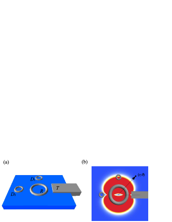
Figure 1: (a) Oblique view of the setup in which a clockwise-moving electron injected into the ring from tunnel junction $T$ fractionalizes into clockwise- and counterclockwise-moving quasiparticles. (b) Top-down view of the same setup with an overlay of a spatial plot of $\overline{\langle B^{2}\rangle}$ predicted for a ring with Luttinger parameter $g=0.2$.

To briefly summarize TLL physics in a ring geometry (see for example, loss ), we consider a one-dimensional system with position $x$ denoting the circumferential direction bounded by $0\leq x<2\pi R$, where $R$ is the radius of the ring. The ring geometry imposes periodic boundary conditions on electron operators such that $\psi(x+2\pi R)=e^{i2\pi\Phi/\Phi_{0}}\psi(x)$ where $\Phi$ is any flux threading the ring and $\Phi_{0}=h/e$. For electrons filling a Fermi sea, we decompose the electron operators as $\psi(x)=\sum_{r}\psi_{r}(x)$ where $\psi_{r}^{\dagger}$ denotes the creation operator for a $r=\pm$ moving electron. The kinetic energy for linearized low-energy modes moving at a Fermi velocity $v_{F}$ takes the form $H_{0}=-iv_{F}\int dx\sum_{r}\psi_{r}^{\dagger}\partial_{x}^{\phantom{\dagger}}\psi_{r}$. As is commonly done, we restrict interaction effects to the short-range form $H_{int}=V\int dx\ \rho^{2}(x)$ where $\rho=e\sum_{r=\pm}\rho_{r}$ is the sum of charge densities $\rho_{r}=\psi_{r}^{\dagger}\psi_{r}^{\phantom{\dagger}}$. Of physical interest, the current operator is given by $\hat{I}=ev_{F}j$, where $j=\sum_{r}r\rho_{r}$.

This model is amenable to a bosonization treatment via the transformation $\psi_{r}(x)\sim e^{irk_{F}x}e^{i\sqrt{\pi}\varphi_{r}(x)}$ giving $\rho_{r}=k_{F}/2\pi+r\partial_{x}\varphi_{r}/\sqrt{2\pi}$, where the chiral bosonic fields $\varphi_{r}$ satisfy the commutation relations $[\varphi_{r}(x),\varphi_{r^{\prime}}(x^{\prime})]=ir\delta_{rr^{\prime}}\mbox{sgn}(x-x^{\prime})$ and $k_{F}$ is the Fermi momentum. The net Hamiltonian $H_{0}+H_{int}$ may be brought into the free TLL form via a Bogoliubov transformation of the $\phi$ fields bosonize , yielding

$$H_{LL}=\frac{u}{4}\int dx\left[\left(\partial_{x}\tilde{\varphi}_{+}\right)^{2}+\left(\partial_{x}\tilde{\varphi}_{-}\right)^{2}\right],$$ (1)

where $u=v_{F}/g$ is the the plasmon velocity, $g$ is the Luttinger parameter $g\equiv 1/\sqrt{1+2V/\pi\hbar v_{F}}$ and $\tilde{\varphi}_{\pm}(x\mp ut)$ are transformed chiral bosons.

The fractionalization of an electron can be seen by representing an electron operator having CW Fermi momentum in terms of the chiral bosons:

$$\psi_{+}^{\dagger}(x,t)\sim e^{-ik_{F}x}e^{-i\frac{\sqrt{\pi}}{2\sqrt{g}}\left[\left(1+g\right)\tilde{\varphi}_{+}(x,t)+\left(1-g\right)\tilde{\varphi}_{-}(x,t)\right]}.$$ (2)

By relating the chiral bosonic fields to the charge and current density operators, $\rho$ and $j$, respectively, it follows that the operator $e^{-i\sqrt{\frac{\pi}{g}}\tilde{\varphi}_{+}(x,0)}$ creates a unit charge $e$ that at time $t$ can be found at position $x-ut$. Thus, we see that the electron operator in Eq. 2 creates the fractional charges $(1\pm g)e/2$ moving in opposite directions. More explicitly, in the situation of interest, the state of the ring after the injection of a CW moving electron at time $t=0$ is given by $|F\rangle=\int\chi(x)\psi_{+}^{\dagger}(x,t=0)dx|G\rangle_{LL}$  leinaas . It is straightforward to calculate the expectation value of the current in this state, $I(x,t)=\langle\hat{I}\rangle_{F}\equiv\langle F|\hat{I}(x,t)|F\rangle$, yielding

$$I(x,t)=\frac{eu}{4\pi R}\left[(1+g)|\chi(x-ut)|^{2}+(1-g)|\chi(x+ut)|^{2}\right].$$ (3)

The form of the current explicitly demonstrates that the electron splinters into two components that rotate in opposite directions, have the same profile $\chi(x)$ and carry charges $(1\pm g)e/2$.

The magnetic field produced by these counter-propagating charges can be evaluated by using the Biot-Savart law to define the magnetic field operator at position ${\bf r}$ as $\hat{\mathbf{B}}=\frac{\mu_{0}}{4\pi}\int d\ell\ \hat{\mathbf{I}}(\ell)\times\mathbf{r}/|\mathbf{r}|^{3}$, where $\mu_{0}$ is permeability of free space. At any given point having polar coordinates $(r,\theta)$ in the plane of the ring, where the origin is at the ring’s center and the electron is inserted at $(R,0)$, the current in Eq. 3 produces a field perpendicular to the plane. For the case of $\chi$ having a spread much smaller than the ring diameter, the $z$-component of the field takes the form

$$\langle\hat{B}_{z}\rangle_{F}=\frac{\mu_{0}e\omega}{2R}\left[(1+g)h(t)-(1-g)h(-t)\right],$$ (4)

where $\omega=u/R$ and $h(t)=(1-a(t))/(\frac{r^{2}}{R^{2}}-2a(t)+1)^{3/2},a(t)=r\cos(\omega t-\theta)/R$. In principle, a time-resolved measurement of the magnetic field, as with other quantities, such as conductance, would yield information on fractionalization. However, as is the goal here, we seek low-frequency or time averaged signatures. Although the tunneling of the electron picks out a specific point on the ring, signatures are effaced by time-averaging of any quantity that is linear in the ring current. For example, $\overline{\langle B_{z}\rangle}$ shows an isotropic spatial profile. (Here, we use the overline to denote time average.)

We thus focus on two measures that are quadratic in the current and can be obtained from a continuous weak linear measurement CWLM via inductive coupling to the ring. The first is simply $S(r,\theta)=\overline{\langle B^{2}_{z}\rangle}$, which can be accessed in a SQUID detector biased to a minimum of its I-V characteristic curve. The second is the average power received by a detector, for example, an ultra-sensitive bolometer. For a small conducting detector (ignoring local spatial variations in the magnetic field), this is given by $P(r,\theta)=\overline{\langle\partial_{t}B_{z}\rangle^{2}}$. Crucially, note that the former involves a quantum average of a quadratic operator and the latter that of a linear operator.

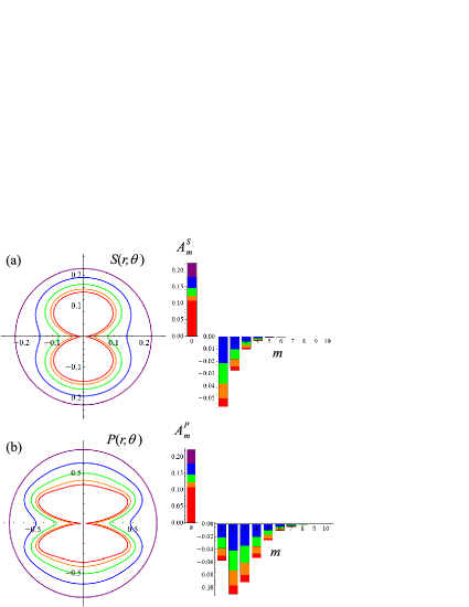
Figure 2: Polar plots of (a) $S(r,\theta)=\overline{\langle B_{z}^{2}(t)\rangle}$ and (b) $P(r,\theta)=\overline{\langle\partial_{t}B_{z}(t)\rangle^{2}}$ at $r=2R$ for values of the Luttinger parameter $g=1.0,\ 0.8,\ 0.6,\ 0.4,\ 0.2$ (from outermost and most isotropic to the innermost) as a function of $\theta$. Bar graphs of the spectral weight of the maps (c) $S$ and (d) $P$ showing the even Fourier coefficients as defined in Eq. 5, i.e., the height of columns for $m=0,1,2$ correspond to the zeroth, $\cos 2\theta$, and $\cos 4\theta$ terms, respectively (the zeroth and non-zeroth coefficients are shown on a different scale). With increasing fractionalization (decreasing $g$), spectral weight is transferred to the non-zeroth coefficients reflecting increasing anisotropy.

The forms of the moments $S$ and $P$ can be easily evaluated by taking appropriate quantum expectations ($\langle\rangle$) and time averages (overline) to obtain $S(r,\theta)=\left(\frac{\mu_{0}e\omega}{2R}\right)^{2}\left[(1+g^{2})\overline{h^{2}(t)}-(1-g^{2})\overline{h(t)h(-t)}\right]$ and a similar form for $\tilde{P}\equiv P/\omega^{2}$ with $h(t)$ replaced by its time derivative $h^{\prime}(t)$. Information on fractionalization is best analyzed by resolving these quantites into their angular Fourier coefficients:

$$S/\tilde{P}(r,\theta)=\left(\frac{\mu_{0}e\omega}{2R}\right)^{2}\sum_{m=0}^{\infty}A^{S/P}_{m}(r)\cos 2m\theta.$$ (5)

In the non-interacting ($g=1$) limit, an electron circles the ring in the CW direction, retaining rotational symmetry on average and thus we have $A^{S/P}_{m}=0,m\neq 0$.

The plots in Fig. 2 capture our central result that higher moments of the current and of the magnetic field profile (in our case, $S$ and $P$) reflect the concurrent motion of fractionalized charge components in their rotational symmetry broken distributions. In the explicit forms of $S$ and $P$ above, given that $\overline{h^{2}(t)}$ preserves rotational symmetry while $\overline{h(t)h(-t)}$ breaks it, we see that primarily $A^{S/P}_{0}$ scale as $1+g^{2}$ and $A^{S/P}_{m\neq 0}$ as $1-g^{2}$. This distribution is illustrated in the plots of Fig.  2 and also agrees with the rotationally symmetric non-interacting limit ($g=1$). The bilateral symmetry of the plots reflects the two charge components moving away from the injection point and towards the diametrically opposite point. That these two special points exist for any arbitrary closed shape suggests that our result that fractionalization causes a distribution that distinguishes two points is robust for any closed loop.

We contrast the behavior of the moments $S$ and $P$ in the fractionalized state to the quantum and classical probabilistic situations. In the quantum state $|QS\rangle$, a superposition of CW and CCW moving electrons, quantum averages of operators that are linear in the current mimic charge fractionalization while their higher moments, (for example, $\langle\hat{B}^{2}_{z}\rangle$)those of linear operators do not. Thus, $S=\overline{\langle\hat{B}^{2}_{z}\rangle}$ is isotropic but $P=\overline{\langle\partial_{t}\hat{B}_{z}\rangle^{2}}$ shows an anisotropic profile similar to that of Fig.  2. b. For the classical situation described by the density matrix $\mathbf{M}_{\rho}$, the moments are evaluated by separately considering CW and CCW electrons and adding their appropriately weighted contributions. Thus, both moments yield isotropic profiles. As summarized in Table. I, the two measurements therefore can distinguish between the three possible scenarios.

In addition to the differences mentioned here, Ref. leinaas distinguishes true fractionalization from other situations by the profound observation that charge fluctuations are in fact a feature of the many-body groundstate and the background of particle-hole excitations while the fractionalized electron is itself ‘sharp’. Translated to our setting, we expect fluctuations in the magnetic field to be induced even by the quiescent TLL ring (having no extra tunneled electron) and identical to those induced by the fractionalized state $|F\rangle$.

Thus far, we have described the injection localized electron wavepacket as a superposition of plasmon-like modes described by Eq. 1. Typically, due to coupling to the environment CedraschiButtiker ; open ; safisaleur , these modes have a finite lifetime, giving rise to a characteristic decoherence time $\tau_{d}$ within which measurements need to be performed. However, for timescales longer than $\tau_{d}$, no plasmons are excited and tunneled electrons need purely be described by the excess electron number, $N=\sum_{r}n_{r}$, and the persistent current due to the number imbalance between CCW- and CW-moving electrons, $J=\sum_{r}rn_{r}$, where we define $n_{r}=r\Phi/\Phi_{0}+\int dx\ \rho_{r}$. The optimal values of these ‘topological’ quantities $N$ and $J$ can be tuned by the application of a gate potential $\mu$ and external flux $\Phi$, and can be determined by minimizing the energy functional derived from Eq. 1kinaret

$$H_{NJ}=\frac{\pi\hbar u}{4\pi R}\left[\frac{1}{g}N^{2}+g\left(J+\frac{2\Phi}{\Phi_{0}}\right)^{2}\right]-\mu N.$$ (6)

The regions of different optimal $N$ and $J$ values can be charted by Coulomb blockade measurements wherein conductance peaks track electron occupation numbers on the ring. We show the boundaries for these regions in (dimensionless) $\mu$-$\Phi$ parameter space in Fig.3. Interactions render these regions to be generically hexagonal, characterized by horizontal sides of length $1-g^{2}$. Thus, the geometry of this diagram is an easily accessible, alternate means of extracting $g$, the Luttinger parameter.

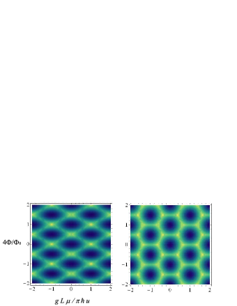
Figure 3: Ground state structure obtained from the Hamiltonian $H_{NJ}$ of Eq. 6. Each cell corresponds to a given electron number ($N$) and persistent current ($J$) which optimizes $H_{NJ}$ as a function of chemical potential (horizontal axis) and magnetic flux (vertical); bright lines indicate a transition in which $J$ or $N$ changes by 1. Cells are (a) diamond shaped for $g=1$ (non-interacting system) and (b) hexagonal shaped for $g(=1/2)\neq 1$ with horizontal side length $1-g^{2}$.

A highlight of this slow-time regime is that it offers another route to distinguishing the fractionalized state $|F\rangle$ by way of persistent current analysis. Ultimately this state is associated with a CW electron and hence has the fixed current value $J=+1$ while the quantum and classical states characterized by $|QS\rangle$ and $\mathbf{M}_{\rho}$ involve CW and CCW electrons, thus showing values $J=\pm 1$ which vary between measurements. Thus, as summarized in Table I, the anisotropy in moment $S$ and non-variability in persistent current distinguish the fractionalized state from the quantum and classical scenarios (though the latter is not a smoking gun test) while anisotropy in the moment $P$ distinguishes classical scenario.

Finally, to provide relevant estimates for experiments, for radius $R\approx 1\ \mu$m and typical circulating frequency $\omega\approx 10^{11}$ Hz, we have $\left(\mu_{0}e\omega/2R\right)^{2}\approx\left(0.1\mbox{ milligauss}\right)^{2}$ and $\left(\mu_{0}e\omega^{2}/2R\right)^{2}\approx\left(80\mbox{ T/sec}\right)^{2}$. An important requirement is that the injection of an electron must be made on a timescale $\tau_{T}\ll 1/\omega$ in order for there to be a ‘clean’ injection of the electron. For the ring, we have $\tau_{T}=R_{T}C$ where $R_{T}$ is the tunnel junction resistance and $C$ ($\sim\epsilon_{0}R\sim 10^{-17}$ F) is the ring capacitance. This gives the requirement that $R_{T}\ll 1\$M$\Omega$. On the other hand, the Coulomb blockade limit holds only if $R_{T}\gg\frac{h}{e^{2}}=26$ k$\Omega$. Thus, we need a $R_{T}\sim 100$ k$\Omega$. Another consideration is that interaction effects at the tunneling point restrict the energy window in which our results hold safisaleur . The role of the electron’s spin can also come into play and can be analyzed by a simple generalization of our results.

In conclusion, we have presented an alternative to the quantum wire based electron-in electron-out paradigm for charge fractionalization in the arena of weak measurements in mesoscopic rings. Our envisioned setup discerns subtle attributes that distinguish fractionalization from quantum and classical probabilistic scenarios and is within the reach of current nanotechnology.

Table 1: Results of various measurements exemplifying how fractionalization ($|F\rangle$) in a TLL can be differentiated from the quantum ($|QS\rangle$) and classical scenarios ($\mathbf{M}_{\rho}$) considered in the text. Time-averaged quantities $S$ and $P$ can display isotropic (I) or anisotropic (AI) distributions. Persistent current measurements can yield non-variable (NV) or variable (V) outcomes for repeated measurements.

	$|F\rangle$	$|QS\rangle$	$\mathbf{M}_{\rho}$
$S(r,\theta)=\langle\hat{B}^{2}_{z}\rangle$	AI	I	I
$P(r,\theta)=\langle\partial_{t}\hat{B}_{z}\rangle^{2}$	AI	AI	I
Persistent Current	NV	V	V

I Acknowledgments

We are grateful to Raffi Budakian and Charles Kane for their perceptive comments. For their support, we thank the NSF under grant DMR 0644022-CAR (W.D. and S.V.), the CAS fellowship at UIUC (S.V.) and the DST, Govt. of India, under a Ramanujan Fellowship (S.L.).

References

- (1) V. V. Deshpande, M. Bockrath, L. I. Glazman, A. Yacoby, Nature 464 209-216 (2010).
- (2) Safi, I and Schulz, H. J. Phys. Rev. B 52, R14265 (1996).
- (3) K.-V. Pham, M. Gabay, and P. Lederer, Phys. Rev B 61, 16397 (2000).
- (4) H. Steinberg et al. Nature Physics 4, 116 (2008).
- (5) D. L. Maslov and M. Stone, Phys. Rev. B 52, R5539 (1995).
- (6) V. V. Ponomarenko, Phys. Rev. B 54, 10328 (1996).
- (7) S. Pugnetti et al. Phys. Rev. B, 79, 035121 (2009).
- (8) J. U. Kim, W.-R. Lee, H.-W. Lee, H.-S. Sim, PRL 102, 076401 (2009).
- (9) K. Le Hur, B. I. Halperin, A. Yacoby, Annals of Physics 323, 3037 (2008).
- (10) Loss, D. PRL 69, 343 (1992).
- (11) M. Stone, Bosonization. World Scientific, Singapore (1994).
- (12) D.V. Averin, Physica C 352, 120, (2001).
- (13) J. M. Leinaas, M. Horsdal, T. H. Hansson, Phys. Rev. B 80, 115327 (2009).
- (14) I. Safi and H. Saleur, PRL 93, 126602 (2004).
- (15) A. H. Castro Neto, C. de C. Chamon, C. Nayak, Phys. Rev. Lett. 79, 4629 (1997).
- (16) P. Cedraschi, V. V. Ponomarenko and M. Buttiker, PRL 84, 346 (2000).
- (17) Kinaret, Jonson, Shekhter, and Eggert. Phys. Rev. B 57, 3777 (1998).