Model Checking with Probabilistic Tabled Logic Programming

Abstract

We present a formulation of the problem of probabilistic model checking as one of query evaluation over probabilistic logic programs. To the best of our knowledge, our formulation is the first of its kind, and it covers a rich class of probabilistic models and probabilistic temporal logics. The inference algorithms of existing probabilistic logic-programming systems are well defined only for queries with a finite number of explanations. This restriction prohibits the encoding of probabilistic model checkers, where explanations correspond to executions of the system being model checked. To overcome this restriction, we propose a more general inference algorithm that uses finite generative structures (similar to automata) to represent families of explanations. The inference algorithm computes the probability of a possibly infinite set of explanations directly from the finite generative structure. We have implemented our inference algorithm in XSB Prolog, and use this implementation to encode probabilistic model checkers for a variety of temporal logics, including PCTL and GPL (which subsumes PCTL^∗). Our experiment results show that, despite the highly declarative nature of their encodings, the model checkers constructed in this manner are competitive with their native implementations.

1 Introduction

Beginning in 1997, we formulated the problem of model checking as one of query evaluation over logic programs [31]. The attractiveness of this approach is that the operational semantics of complex process languages (originally CCS [23], followed by value-passing calculi [32], the pi-calculus [24], and mobile calculi with local broadcast [41]), as well as the semantics of complex temporal logics (e.g., the modal mu-calculus [20]), can be expressed naturally and at a high level as clauses in a logic program. Model checking over these languages and logics then becomes query evaluation over the logic programs that directly encode their semantics.

The past two decades have witnessed a number of important developments in Probabilistic Logic Programming (PLP), combining logical and statistical inference, and leading to a number of increasingly mature PLP implementations. A natural question is whether the advances in PLP enable the development of model checkers for probabilistic systems, the same way traditional LP methods such as tabled evaluation and constraint handling enabled us to formulate model checkers for a variety of non-probabilistic systems.

It turns out that existing PLP inference methods are not sufficiently powerful to be used as a basis for probabilistic model checking. One of the earliest PLP inference procedures, used in PRISM [40], is formulated in terms of the set of explanations of answers. PRISM puts in place three restrictions to make its inference work: (a) independence: random variables used in any single explanation are all independent; (b) mutual exclusion: two distinct explanations of a single answer are mutually exclusive; and (c) finiteness: the number of possible explanations of an answer is finite. Subsequent systems, notably ProbLog [4] and PITA [35] have eliminated the independence and mutual exclusion restrictions of PRISM. This, however, is still insufficient for model checking, as the following example shows.

% 3 "switches" (random processes) for transitions % from states s0, s1 and s4, respectively. values(t(s0), [s0, s1, s2]). values(t(s1), [s1, s3, s4]). values(t(s4), [s3]). % Distribution parameters of the random variables. set_sw(t(s0), [.5, .3, .2]). set_sw(t(s1), [.4, .1, .5]). set_sw(t(s4), [1]). % Transition from S at instance I goes to T, % as determined by the corresponding random process. trans(S, I, T) :- msw(t(S), I, T). % Starting at state S at instance I, state T is reachable. reach(S, I, T) :- trans(S, I, U), reach(U, next(I), T). reach(S, _, S).

(a)

(b)

Figure 1: (a) Example Markov chain; (b) PRISM encoding of transitions in the chain.

Motivating Example:

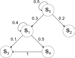
Figure 1 shows a Markov chain and its representation in PRISM. Note that the behavior of a Markov chain is memoryless: in any execution of the chain, a transition from state, say $s$, is independent of any previous transitions (including those from the same state). The definition of the trans predicate has an explicit instance parameter I, which is subsequently used in msw. PRISM treats different instances of the same random variable as independent. Thus trans correctly encodes the semantics of the Markov chain.

We first consider simple reachability questions of the form: What is the likelihood that on an execution of the chain from a start state $s$, a final state $t$ will be reached? The reachability question using the reach predicate is defined in Figure 1(b). Consider the likelihood of reaching state s3 from s0. This query can be posed as the predicate prob(reach(s0, 0, s3), P), where prob/2 finds the probability of answers (P) to a given query reach(s0,0,s3).

The query prob(reach(s0,0,s3),P) cannot be evaluated in PRISM. We illustrate this by first describing PRISM’s inference at a high level. In PRISM, inference of probabilities proceeds in the same way as logical inference, except when the selected literal is an msw. In this case, the inference procedure enumerates the values of the random variable, and continues the inference for each value (by backtracking). The probability of a derivation is simply the product of the probabilities of the random variables (msw outcomes) used in that derivation (under the independence assumption). The probability of a query answer is the sum of probabilities of the set of all derivations for that answer (using the mutual-exclusiveness and finiteness assumptions). Note that reach(s0,0,s3) has infinitely many derivations, and hence PRISM cannot infer its probability.

Markov chains can be encoded in ProbLog and LPAD [44] in a similar manner. As is the case for PRISM, however, analogous reachability queries cannot be evaluated in these systems either. The sequence of random-variable valuations used in the derivation of an answer is called an explanation. In contrast to PRISM, ProbLog [4] and PITA [35], which is an implementation of LPAD, materialize the set of explanations of an answer in the form of a BDD. Probabilities are subsequently computed based on the BDD. This approach permits these systems to correctly infer probabilities even when the independence and mutual-exclusion assumptions are violated. Note that in the evaluation of reach, when a state is encountered, the next state is determined by a fresh random process. Hence, the set of explanations of reach(s0,0,s3) is infinite. Since BDDs can only represent finite sets, the probability of reach(s0,0,s3) cannot be computed in ProbLog or LPAD.

To correctly infer the probability of reach(s0,0,s3), we need an algorithm that works even when the set of explanations is infinite. Moreover, it is easy to construct queries where the independence and mutual exclusion properties do not hold. For example, consider the problem of inferring the probability of reaching s3 or s4 (i.e., the query reach(s0,0,s3); reach(s0,0,s4)). Since some paths to s3 pass through s4, explanations for reach(s0,0,s3) and reach(s0,0,s4) are not mutually exclusive. The example of Fig. 1 illustrates that to build model checkers based on PLP, we need an inference algorithm that works even when the finiteness, mutual-exclusion and independence assumptions are simultaneously violated.

Summary of Contributions:

In this paper, we present PIP (for “Probabilistic Inference Plus”), a new algorithm for inferring probabilities of queries in a probabilistic logic program. PIP is applicable even when explanations are not necessarily mutually exclusive or independent, and the number of explanations is infinite. We demonstrate the utility of this new inference algorithm by constructing model checkers for a rich class of probabilistic models and temporal logics (see Section 5). Our model checkers are based on high-level, logical encodings of the semantics of the process languages and temporal logics, thus retaining the highly declarative nature of our prior work on model checking non-probabilistic systems.

We have implemented our PIP inference algorithm in XSB Prolog [42]. Our experimental results show that, despite the highly declarative nature of our encodings of the model checkers, their performance is competitive with their native implementations.

The rest of this paper develops along the following lines. Section 3 provides requisite background on probabilistic logic programming. Section 4 presents our PIP algorithm. Section 5 describes our PLP encodings of probabilistic model checkers, while Section 6 contains our experimental evaluation. Section 7 offers our concluding remarks and directions for future work.

2 Related Work

There is a substantial body of prior work on encoding complex model checkers as logic programs. These approaches range from using constraint handling to represent sets of states such as those that arise in timed systems [12, 6, 27, 29], data-independent systems [39] and other infinite-state systems [5, 26]; tabling to handle fixed point computation [33, 8]; procedural aspects of proof search to handle name handling [47] and greatest fixed points [11]. However, all these works deal only with non-probabilistic systems.

With regard to related work on probabilistic inference, Statistical Relational Learning (SRL) has emerged as a rich area of research into languages and techniques for supporting modeling, inference and learning using a combination of logical and statistical methods [10]. Some SRL techniques, including Bayesian Logic Programs (BLPs) [18], Probabilistic Relational Models (PRMs) [9] and Markov Logic Networks (MLNs) [34], use logic to compactly represent statistical models. Others, such as PRISM [40], Stochastic Logic Programs (SLP) [25], Independent Choice Logic (ICL) [30], CLP(BN) [38], ProbLog [4], LPAD [44] and CP-Logic [43], define inference primarily in logical terms, subsequently assigning statistical properties to the proofs. Motivated primarily by knowledge representation problems, these works have been naturally restricted to cases where the models and the inference proofs are finite. Recently, a number of techniques have generalized these frameworks to handle random variables that range over continuous domains (e.g. [19, 28, 45, 13, 14, 16]), but still restrict proof structures to be finite.

Modeling and analysis of probabilistic systems, both discrete- and continuous-time, has been an actively researched area. Probabilistic Computation Tree Logic (PCTL) [15] is a widely used temporal logic for specifying properties of discrete-time probabilistic systems. PCTL^∗ [1] is a probabilistic extension of LTL and is more expressive than PCTL. Generalized Probabilistic Logic (GPL) [3] is a probabilistic variant of the modal mu-calculus. The Prism model checker [22] is a leading tool for modeling and verifying a wide variety of probabilistic systems: Discrete- and Continuous-Time Markov chains and Markov Decision Processes. There is also prior work on techniques for verifying more expressive probabilistic systems, including Recursive Markov chains (RMCs) [7] and Probabilistic Push-Down systems [21], both of which exhibit context-free behavior. The probability of reachability properties in such systems is computed as the least solution to a corresponding set of monotone polynomial equations. PReMo [46] is a model checker for RMCs. Reactive Probabilistic Labeled Transition Systems (RPLTS) [3] generalize Markov chains by adding external choice (multiple labeled actions). GPL properties of such systems are also computed as the least (or greatest, based on the property) solution to a set of monotone polynomial equations. To the best of our knowledge, this paper presents the first implementation of a GPL model checker.

3 Preliminaries

Notations:

The root symbol of a term $t$ is denoted by $\pi(t)$ and its $i$-th subterm by $\arg_{i}(t)$. Following traditional LP notation, a term with a predicate symbol as root is called an atom. The set of variables in a term $t$ is denoted by $\mbox{\it vars\/}(t)$. A term $t$ is ground if $\mbox{\it vars\/}(t)=\emptyset$.

Following PRISM, a probabilistic logic program (PLP) is of the form $P=P_{F}\cup P_{R}$, where $P_{R}$ is a definite logic program, and $P_{F}$ is the set of all possible msw/3 atoms. The set of possible msw atoms and the distribution of their subsets is given by values and set_sw directives, respectively. For example, clauses trans and reach in Fig. 1(b) are in $P_{R}$. The set $P_{F}$ of that program contains msw atoms such as msw(t(s0), 0, s0), msw(t(s0),next(0), s0), msw(t(s0), 0, s1), $\ldots$, msw(t(s1),next(0), s1), $\ldots$.

In an atom of the form $\mbox{\tt msw}(t_{1},t_{2},t_{3})$, $t_{1}$ is a term representing a random process (switch in PRISM terminology), $t_{2}$ is an instance and $t_{3}$ is the outcome of the process at that instance. According to PRISM semantics, two msw atoms with distinct processes are independent; and two msw atoms with distinct instances (even if they have the same process) are independent. Two msw atoms with the same process and instance but different outcomes are mutually exclusive.

4 The Inference Procedure PIP

A key idea behind the PIP inference algorithm is to represent the (possibly infinite) set of explanations in a symbolic form. Observe from the example in Fig. 1 that, even though the set of paths (each with its own distinct probability) from state s0 to state s3 is infinite, the regular expression $\mbox{\tt s0}^{+}\mbox{\tt s1}^{*}\mbox{\tt s4}^{?}\mbox{\tt s3}$ captures this set exactly. Following this analogy, we devise a grammar-based notation that can succinctly represent infinite sets of finite sequences.

Definition 1 (Explanation)

An explanation of an atom $A$ with respect to a PLP $P=P_{F}\cup P_{R}$ is a set $\xi\subseteq P_{F}$ of msw atoms such that (i) $\xi,P_{R}\vdash A$ and (ii) $\xi$ is consistent, i.e. it contains no pair of mutually exclusive msw atoms.

The set of all explanations of $A$ w.r.t. $P$ is denoted by ${\cal E}_{P}(A)$. $\Box$

Example 1 (Set of explanations)

Consider the PLP of Fig. 1(b). The set of explanations for reach(s0,0,s3) is:

$$\begin{array}[]{l}\mbox{\tt msw}(t(s0),0,s1),\ \mbox{\tt msw}(t(s1),\mbox{\it next\/}(0),s3).\\ \mbox{\tt msw}(t(s0),0,s0),\ \mbox{\tt msw}(t(s0),\mbox{\it next\/}(0),s1),\ \mbox{\tt msw}(t(s1),\mbox{\it next\/}(\mbox{\it next\/}(0)),s3).\\ \vdots\\ \mbox{\tt msw}(t(s0),0,s1),\ \mbox{\tt msw}(t(s1),\mbox{\it next\/}(0),s1),\ \mbox{\tt msw}(t(s1),\mbox{\it next\/}(\mbox{\it next\/}(0)),s3).\\ \vdots\end{array}$$

4.1 Representing Explanations

As Example 1 illustrates, a representation in which instance identifiers are explicitly captured will not be nearly as compact as the corresponding regular expression (shown earlier). On the other hand, a representation (like the regular expression) that completely ignores instance identifiers will not be able to identify identical instances of a random process nor properly distinguish distinct ones.

We solve this problem by observing that in PRISM’s semantics, different instances of the same random process are independent and identically distributed (i.i.d.). Consequently, the probability of reach(s0,0,s3) (reaching s3 from s0 starting at instance 0), is the same as that of reach(s0,next(0),s3) (starting at instance 1), which is the same as that of reach(s0,H,s3), for any instance H. Consequently, it is sufficient to infer probabilities for a single parameterized instance. Below, we formalize the set of PLP programs for which such an abstraction is possible.

Definition 2 (Temporal PLP)

A temporal probabilistic logic program is a probabilistic logic program $P$ with declarations of the form temporal($p/n-i$), where $p/n$ is an $n$-ary predicate, and $i$ is an argument position (between 1 and $n$) called the instance argument of $p/n$ . Predicates $p/n$ in such declarations are called temporal predicates. $\Box$

The set of temporal predicates in a temporal PLP $P$ is denoted by ${\mathtt{temporal}(P)}$; the set of all predicates in $P$ is denoted by ${\mathtt{preds}(P)}$. By convention, every temporal PLP contains an implicit declaration temporal(msw/3-2), indicating that msw/3 is a temporal predicate, and its second argument is its instance argument. The instance argument of a predicate $p/n$ is denoted by $\chi(p/n)$. For example, the program of Fig. 1(b) becomes a temporal PLP when temporal(trans/3-2) and temporal(reach/3-2) are added. For this program, ${\mathtt{temporal}(P)}=\{\mathtt{reach/3},\mathtt{trans/3},\mathtt{msw/3}\}$, and $\chi(\mathtt{reach/3})=\chi(\mathtt{trans/3})=\chi(\mathtt{msw/3})=2$.

We extend the notion of instance argument from predicates to atoms as follows. Let $\alpha$ be an atom in a temporal PLP such that its root symbol is a temporal predicate, i.e., $\pi(\alpha)\in{\mathtt{temporal}(P)}$. Then the instance of $\alpha$, denoted by $\chi(\alpha)$ by overloading the symbol $\chi$, is $\arg_{\chi(\pi(\alpha))}(\alpha)$. We also denote, by $\overline{\chi}(\alpha)$, a term constructed by omitting the instance of $\alpha$; i.e. if $\alpha=f(t_{1},\ldots,t_{i-1},t_{i},t_{i+1},\ldots t_{n})$ and $\chi(\alpha)=t_{i}$, then $\overline{\chi}(\alpha)=f(t_{1},\ldots,t_{i-1},t_{i+1},\ldots t_{n})$.

Explanations of a temporal PLP can be represented by a notation similar to Definite Clause Grammars (DCGs).

Example 2 (Set of explanations using DCG notation)

Considering again the program of Fig. 1(b), the set of explanations for reach(s0,H,s3) can be succinctly represented by the following DCG:

$$\begin{array}[]{l}\mbox{\tt expl}(\mbox{\tt reach}(s0,s3),H)\longrightarrow[\mbox{\tt msw}(t(s0),H,s0)],\mbox{\tt expl}(\mbox{\tt reach}(s0,s3),next(H)).\\ \mbox{\tt expl}(\mbox{\tt reach}(s0,s3),H)\longrightarrow[\mbox{\tt msw}(t(s0),H,s1)],\mbox{\tt expl}(\mbox{\tt reach}(s1,s3),next(H)).\\ \mbox{\tt expl}(\mbox{\tt reach}(s1,s3),H)\longrightarrow[\mbox{\tt msw}(t(s1),H,s1)],\mbox{\tt expl}(\mbox{\tt reach}(s1,s3),next(H)).\\ \mbox{\tt expl}(\mbox{\tt reach}(s1,s3),H)\longrightarrow[\mbox{\tt msw}(t(s1),H,s3)],\mbox{\tt expl}(\mbox{\tt reach}(s1,s3),next(H)).\\ \mbox{\tt expl}(\mbox{\tt reach}(s1,s3),H)\longrightarrow[\mbox{\tt msw}(t(s1),H,s4)],\mbox{\tt expl}(\mbox{\tt reach}(s4,s3),next(H)).\\ \mbox{\tt expl}(\mbox{\tt reach}(s3,s3),H)\longrightarrow[].\\ \mbox{\tt expl}(\mbox{\tt reach}(s4,s3),H)\longrightarrow[\mbox{\tt msw}(t(s4),H,s3)],\mbox{\tt expl}(\mbox{\tt reach}(s3,s3),next(H)).\\ \end{array}$$

Note that each expl generates a sequence of msws. For this example, it is also the case that in a string generated from $\mbox{\tt expl}(\mbox{\tt reach}(s0,s3),H)$, the msws all have instances equal to or later than H. It is then immediate that msw(t(s0), H, s0) is independent of any msw generated from $\mbox{\tt expl}(\mbox{\tt reach}(s0,s3),next(H))$. This property holds for an important subclass called temporally well-formed programs, defined as follows.

Definition 3 (Temporally Well-Formed PLP)

A temporal PLP $P$ is said to be temporally well formed if for each clause $(\alpha\ \mbox{${:\!\!-\;}$}\beta_{1},\ldots\beta_{n})\in P$:

• If $\pi(\alpha)\in{\mathtt{temporal}(P)}$ then $\forall\ i,1\leq i\leq n,\mbox{ s.t. }\pi(\beta_{i})\in{\mathtt{temporal}(P)}$, $\chi(\beta_{i})$ contains $\chi(\alpha)$, and $\mbox{\it vars\/}(\beta_{i})=\mbox{\it vars\/}(\alpha)$.

• If $\pi(\alpha)\not\in{\mathtt{temporal}(P)}$ then there is at most one $i$, $1\leq i\leq n$ s.t. $\pi(\beta_{i})\in{\mathtt{temporal}(P)}$.

• Instance arguments $\chi(\alpha)$ or $\chi(\beta_{i})$ or their subterms are unified only with other instance arguments, their subterms, or with ground terms. $\Box$

For temporally well-formed programs, the explanations for an atom can be represented succinctly by DCGs. Such DCGs are called explanation generators.

Definition 4 (Explanation Generator)

Let $P$ be a temporally well-formed PLP and let $Q$ be a query such that all non-instance-arguments of $Q$ are ground (i.e. $\overline{\chi}(Q)$ is ground). Then, an explanation generator for $Q$ with respect to $P$ is a DCG $\Gamma$, with non-terminals of the form $\mbox{\tt expl}(G,H)$ and terminals of the form $\mbox{\tt msw}(r,H,v)$ such that:

• For every production $(\beta_{0}\rightarrow\beta_{1},\ldots,\beta_{n})\in\Gamma$, $\forall\ i$, $0\leq i\leq n$, all non-instance-arguments of $\beta_{i}$ are ground; i.e., if $\beta_{i}=\mbox{\tt expl}(G,H)$, then $G$ is ground, and if $\beta_{i}=\mbox{\tt msw}(r,H,v)$, then $r$ and $v$ are ground.

• ${\cal E}_{P}(Q)$, the set of explanations for $Q$ w.r.t. $P$, is identical to the language of $\Gamma$ with $\mbox{\tt expl}(\overline{\chi}(Q),\chi(Q))$ as the start symbol. $\Box$

The DCG in Example 2 is the explanation generator for the query reach(s0,H,s3) over the program given in Figure 1(b). In general, an explanation generator may not be in a form from which we can directly infer the probabilities. For this purpose, we use the factoring algorithm described below.

4.2 Factored Explanation Diagrams

The factored form of an explanation generator is obtained by constructing a Factored Explanation Diagram (FED), whose structure closely follows that of a BDD. Similar to a BDD, a FED is a labeled direct acyclic graph with two distinguished leaf nodes: tt, representing true, and ff, representing false. While the internal nodes of a BDD are Boolean variables, a FED contains two kinds of internal nodes: one representing terminal symbols of explanations (msws), and the other representing non-terminal symbols of explanations (expls). We use a partial order among nodes, denoted by “$<$”, to construct a FED.

Definition 5 (Factored Explanation Diagram)

A factored explanation diagram (FED) is a labeled directed acyclic graph with:

• Four kinds of nodes: tt, ff, $\mbox{\tt msw}(r,h)$ and $\mbox{\tt expl}(t,h)$, where $r$ is a ground term representing a random process, $t$ is a ground term, and $h$ is an instance term;

• Nodes tt and ff are 0-ary, and occur only at leaves of the graph;

• $\mbox{\tt msw}(r,h)$ is an $n$-ary node when $r$ is random process with $n$ outcomes, and the edges to the $n$ children are labeled with the possible outcomes of $r$;

• $\mbox{\tt expl}(t,h)$ is a binary node, and the edges to the children are labeled $0$ and $1$.

• If there is an edge from node $x_{1}$ to $x_{2}$, then $x_{1}<x_{2}$. $\Box$

Note that the multi-valued decision diagrams used in the implementation of PITA [36] are a special case of FEDs with only tt, ff and $\mbox{\tt msw}(r,h)$ nodes, where $r$ and $h$ are ground.

We represent non-trivial FEDs by $x?\mbox{\it Alts\/}$, where $x$ is the node and Alts is the list of edge-label/child pairs. For example, a FED $F$ whose root is an MSW node is written as $\mbox{\tt msw}(r,h)?[{v_{1}\!\!:\!\!F_{1}},{v_{2}\!\!:\!\!F_{2}},\ldots,{v_{n}\!\!:\!\!F_{n}}]$, where $F_{1},F_{2},\ldots,F_{n}$ are children FEDs (not all necessarily distinct) and $v_{1},v_{2},\ldots,v_{n}$ are possible outcomes of the random process $r$ such that $v_{i}$ is the label on the edge from $F$ to $F_{i}$. Similarly, a FED $F$ whose root is an EXPL node is written as $\mbox{\tt expl}(t,h)?[{0\!\!:\!\!F_{0}},{1\!\!:\!\!F_{1}}]$, where $F_{0}$ and $F_{1}$ are the children of $F$ with edge labels $0$ and $1$, respectively.

We now define the ordering relation “$<$” among nodes. We first define a time order “$\prec$” among instances such that $h_{1}\prec h_{2}$ if $h_{1}$ represents an earlier time instant than $h_{2}$. If $h_{1}\not\preceq h_{2}$ and $h_{2}\not\preceq h_{1}$, then $h_{1}$ and $h_{2}$ are incomparable, denoted as $h_{1}\sim h_{2}$. We also assume an arbitrary order $<$ among terms.

Definition 6 (Node order)

Let $x_{1}$ and $x_{2}$ be nodes in a FED. Then $x_{1}<x_{2}$ if it matches one of the following cases:

• $\mbox{\tt msw}(r_{1},h_{1})<\mbox{\tt msw}(r_{2},h_{2})$ if $h_{1}\prec h_{2}$ or ($r_{1}<r_{2}$ and ($h_{1}=h_{2}$ or $h_{1}\sim h_{2}$))

• $\mbox{\tt msw}(r_{1},h_{1})<\mbox{\tt expl}(t_{2},h_{2})$ if $h_{1}\prec h_{2}$ or $h_{1}\sim h_{2}$

• $\mbox{\tt expl}(t_{1},h_{1})<\mbox{\tt expl}(t_{2},h_{2})$ if $t_{1}<t_{2}$ and $h_{1}\sim h_{2}$. $\Box$

Proposition 1 (Independence and Node Order)

For any nodes $x_{1}$, $x_{2}$ in an FED, if $x_{1}<x_{2}$ or $x_{2}<x_{1}$, then $x_{1}$ and $x_{2}$ are independent.

Definition 7 (Binary Operations on FEDs)

$F_{1}\oplus F_{2}$, where $\oplus\in\{\land,\lor\}$ is a FED $F$ derived as follows:

• $F_{1}$ is tt, and $\oplus=\lor$, then $F=\mbox{\tt tt}$.

• $F_{1}$ is tt, and $\oplus=\land$, then $F=F_{2}$.

• $F_{1}$ is ff, and $\oplus=\land$, then $F=\mbox{\tt ff}$.

• $F_{1}$ is ff, and $\oplus=\lor$, then $F=F_{2}$.

• $F_{1}=x_{1}?[{v_{1,1}\!\!:\!\!F_{1,1}},\ldots,{v_{1,n_{1}}\!\!:\!\!F_{1,n_{1}}}]$, $F_{2}=x_{2}?[{v_{2,1}\!\!:\!\!F_{2,1}},\ldots,{v_{2,n_{2}}\!\!:\!\!F_{2,n_{2}}}]$:

  c1.

  $x_{1}<x_{2}$: $F=x_{1}?[{v_{1,1}\!\!:\!\!(F_{1,1}\oplus F_{2})},\ldots,{v_{1,n_{1}}\!\!:\!\!(F_{1,n_{1}}\oplus F_{2})}]$

  c2.

  $x_{1}=x_{2}$: $F=x_{1}?[{v_{1,1}\!\!:\!\!(F_{1,1}\oplus F_{2,1})},\ldots,{v_{1,n_{1}}\!\!:\!\!(F_{1,n_{1}}\oplus F_{2,n_{1}})}]$

  c3.

  $x_{1}>x_{2}$: $F=x_{2}?[{v_{2,1}\!\!:\!\!(F_{1}\oplus F_{2,1})},\ldots,{v_{2,n_{2}}\!\!:\!\!(F_{1}\oplus F_{2,n_{2}})}]$

  c4.

  $x_{1}\not<x_{2},x_{2}\not<x_{1}$: $F=\mbox{\tt expl}(\mbox{\tt merge}(\oplus,F_{1},F_{2}),h)?[{0\!\!:\!\!\mbox{\tt ff}},{1\!\!:\!\!\mbox{\tt tt}}]\quad$ where $h$ is the common part of instances of $x_{1}$ and $x_{2}$.  $\Box$

Note that Def. 7 is a generalization of the corresponding operations on BDDs. Also, when $x_{1}$ and $x_{2}$ are both msw nodes, since $<$ defines a total order between them, case c4 will not apply. When the operand nodes cannot be ordered (case c4), we generate a placeholder (a merge node) indicating the operation to be performed. Such placeholders will be expanded when FEDs are built from an explanation generator (see Def. 8 below). Note that merge nodes may be generated only if one or both arguments is a FED rooted at an expl node.

We now give a procedure for constructing FEDs from an explanation generator for query $Q$ with respect to program $P$.

Definition 8 (Construction of Factored Explanation Diagrams)

Given an explanation generator $\Gamma$, $F$ is a FED corresponding to goal $G$ if $\mbox{\tt fed}(G,F)$ holds, where fed_c is the smallest relation and $E$ is the smallest set such that:

• $\mbox{\tt fed\_c}(\beta_{0},F)$ holds whenever $\{(\beta_{0}\rightarrow\beta_{1,1},\ldots,\beta_{1,n_{1}}),$ $(\beta_{0}\rightarrow\beta_{2,1},\ldots,\beta_{2,n_{2}}),$ $\ldots,$ $(\beta_{0}\rightarrow\beta_{k,1},\ldots,\beta_{k,n_{k}})\}$ is the set of all clauses in $P$ with $\beta_{0}$ on the left hand side, and

  $$F=\bigvee_{i=1}^{k}\quad\bigwedge_{j=1}^{n_{k}}\quad F_{i,j}\quad\quad\mbox{where}\ F_{i,j}\ \mbox{is such that}\ \mbox{\tt fed}(\beta_{i,j},F_{i,j})\ \mbox{holds}$$

• $\mbox{\tt fed\_c}(\beta_{0},F)$ holds whenever $\beta_{0}=\mbox{\tt merge}(\oplus,F_{1},F_{2})\in E$, and

  • $F_{1}=\mbox{\tt expl}(t_{1},h_{1})?[{0\!\!:\!\!F_{1,0}},{1\!\!:\!\!F_{1,1}}]$,  $\mbox{\tt fed}(\mbox{\tt expl}(t_{1},h_{1}),F_{1}^{\prime})$ holds,
    and $F=\oplus(F_{1}^{\prime}[\mbox{\tt ff}\mapsto F_{1,0},\mbox{\tt tt}\mapsto F_{1,1}],F_{2})$.

  • $F_{2}=\mbox{\tt expl}(t_{2},h_{2})?[{0\!\!:\!\!F_{2,0}},{1\!\!:\!\!F_{2,1}}]$,  $\mbox{\tt fed}(\mbox{\tt expl}(t_{2},h_{2}),F_{2}^{\prime})$ holds,
    and $F=\oplus(F_{1},F_{2}^{\prime}[\mbox{\tt ff}\mapsto F_{2,0},\mbox{\tt tt}\mapsto F_{2,1}])$.

• $\mbox{\tt fed}(G,F)$ holds whenever

  • $G=\mbox{\tt msw}(r,h,v)$ and $F=\mbox{\tt msw}(r,h)?[{v_{1}\!\!:\!\!F_{1}},\ldots{v_{n}\!\!:\!\!F_{n}}]$ where for all $i$, $F_{i}=\mbox{\tt tt}$ if $v_{i}=v$ and $F_{i}=\mbox{\tt ff}$ otherwise.

  • $G=\mbox{\tt expl}(t,h)$, $h$ is neither a ground term nor a variable,
    and $F=\mbox{\tt expl}(t,h)?[{0\!\!:\!\!\mbox{\tt ff}},{1\!\!:\!\!\mbox{\tt tt}}]$.

  • $G=\mbox{\tt expl}(t,h)$, $h$ is either ground or a variable, and $F=\lor_{\mbox{\tt fed\_c}(G,F^{\prime})}F^{\prime}$.

• $\mbox{\tt merge}(\oplus,F_{1},F_{2})\in E$ whenever there is some $G,F$ such that $\mbox{\tt fed}(G,F)$ holds, and there is a node in $F$ of the form $\mbox{\tt expl}(\mbox{\tt merge}(\oplus,F_{1},F_{2}),h)$.  $\Box$

The above definition is inductive, and can be turned into a tabled logic program implementing the construction procedure. Furthermore, FEDs are maintained using a dictionary to ensure that the FEDs have a DAG instead of tree structure.

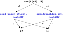
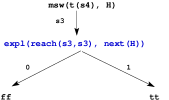
Example 3

Three of the four FEDs for the explanation generator in Example 2 are shown in Fig. 2. The FED for expl(reach(s3,s3),H), not shown in the figure, is tt.

(a) FED for expl(reach(s0,s3),H) (c) FED for expl(reach(s4,s3),H)

(b) FED for expl(reach(s1,s3),H)

Figure 2: FEDs for Example 2

4.3 Computing Probabilities from FEDs

A factored explanation diagram can be viewed as a stochastic grammar. Following [7], we can generate a set of simultaneous equations from the stochastic grammar, and find the probability of the language from the least solution of the equations. The generation of equations from the factored representation of explanations is formalized below.

Definition 9 (Temporal Abstraction)

Given a temporal PLP $P$, the temporal abstraction of a term $t$, denoted by ${\mathtt{abs}}(t)$ is $\overline{\chi}(t)$ if $\pi(t)\in{\mathtt{temporal}(P)}$, and $\chi(t)$ is non-ground; and $t$ otherwise. That is, for a term $t$ with a temporal predicate as root, ${\mathtt{abs}}(t)$ replaces its instance argument with a special symbol $\bot$ if that argument is not ground. $\Box$

Definition 10 (Distribution)

Let $\rho$ be a random process specified in a PLP $P$. The set of values produced by $\rho$ is denoted by $\mbox{\tt values}_{P}(\rho)$. The distribution of $\rho$, denoted by $\mbox{\tt distr}_{P}(\rho)$, is a function from the set of all terms over the Herbrand Base of $P$ to $[0,1]$ such that $\sum_{v\in\mbox{\tt values}_{P}(\rho)}\mbox{\tt distr}_{P}(\rho)(v)=1$ $\Box$

Definition 11 (System of Equations for PLP)

Let $\Gamma$ be an explanation generator, fed be the relation defined in Def. 8, $V$ be a countable set of variables, and $f$ be a one-to-one function from terms to $V$. The system of polynomial equations $E_{(\Gamma,V,f)}$ $=\{(f({\mathtt{abs}}(G))={\cal P}(F))\mid\mbox{\tt fed(G,F)}\mbox{ holds}\}$, where ${\cal P}$ is a function that maps FEDs to polynomials, is defined as follows:

$$\begin{array}[]{rcl}{\cal P}(\mbox{\tt ff})&=&0\\ {\cal P}(\mbox{\tt tt})&=&1\\ {\cal P}(\mbox{\tt msw}(r,h)?[{v_{1}\!\!:\!\!F_{1}},\ldots,{v_{n}\!\!:\!\!F_{n}}])&=&\sum_{i=1}^{n}\mbox{\tt distr}(r)(v)*{\cal P}(F_{i})\\ {\cal P}(\mbox{\tt expl}(t,h)?[{0\!\!:\!\!F_{0}},{1\!\!:\!\!F_{1}}])&=&f({\mathtt{abs}}(\mbox{\tt expl}(t,h)))*{\cal P}(F_{1})\\ &&\quad+(1-f({\mathtt{abs}}(\mbox{\tt expl}(t,h))))*{\cal P}(F_{0})\\ \end{array}$$

The set of equations for Example 3 is shown in Fig. 3.

The implementation of the above definition is such that shared FEDs result in shared variables in the equation system, thereby ensuring that every FED is evaluated at most once. The correspondence between a PLP in factored form and the set of monotone equations permits us to compute the probability of query answers in terms of the least solution to the system of equations.

$\begin{array}[]{l@{\extracolsep{5em}}ll}\hline\cr x_{0}=t_{00}*x_{0}+t_{01}*x_{1}&t_{00}=.5&t_{14}=.5\\ x_{1}=t_{11}*x_{1}+t_{13}*x_{3}+t_{14}*x_{4}&t_{01}=.3&t_{43}=1\\ x_{3}=1&t_{11}=.4&\\ x_{4}=t_{43}*x_{3}&t_{13}=.1&\\ \hline\cr\end{array}$

Figure 3: Set of equations generated from the set of FEDs of Example 3

Theorem 2 (Factored Forms and Probability)

Let $\Gamma$ be an explanation generator for query $Q$ w.r.t. program $P$. Let $V$ be a set of variables and let $f$ be a one-to-one function from terms to $V$. Then, $X$ is the probability of a query answer $Q$ evaluated over $P$, denoted by $\mathtt{prob}(Q,X)$, if $X$ is the value of the variable $f(\mbox{\tt expl}(\overline{\chi}(Q),\chi(Q)))$ in the least solution of the corresponding set of equations, $E_{(\Gamma,V,f)}$.

The proof of the above theorem can be obtained by treating the explanations in $P$ as strings generated by a corresponding stochastic CFG. Such a correspondence is possible since the explanations are represented in factored form. The following properties show that the algorithm for finding probabilities of a query answer is well defined.

Proposition 3 (Monotonicity)

If $\Gamma$ is a definite PLP in factored form, $V$ is a set of variables and $f$ is a one-to-one function as required by Def. 11, then the system of equations $E_{(\Gamma,V,f)}$ is monotone in $[0,1]$.

Monotone systems have the following important property:

Proposition 4 (Least Solution [7])

Let $E$ be a set of polynomial equations which is monotone in $[0,1]$. Then $E$ has a least solution in $[0,1]$. Furthermore, a least solution can be computed to within an arbitrary approximation bound by an iterative procedure.

Note that FEDs are non-regular since expl nodes may have other expl nodes as children, and hence the resulting equations may be non-linear. Proposition 4 establishes that probability of query answers can be effectively computed even when the set of equations is non-linear.

The probability of the language of explanations in Example 2 (via the equations in Fig. 3) is given by the value of $x_{0}$ in the least solution, which is $0.6$.

5 Applications

We now present two model checkers that demonstrate the utility of the new PIP inference technique.

PCTL:

The syntax of an illustrative fragment of PCTL is given by:

$$\begin{array}[]{rl}\mbox{\it SF\/}\Coloneqq&\mbox{\tt prop}(A)\ |\ \mbox{\tt neg}(\mbox{\it SF\/})\ |\ \mbox{\tt and}(\mbox{\it SF\/}_{1},\mbox{\it SF\/}_{2})|\ \mbox{\tt pr}(\mbox{\it PF\/},\mbox{\tt gt},B)\ |\ \mbox{\tt pr}(\mbox{\it PF\/},\mbox{\tt geq},B)\\ \mbox{\it PF\/}\Coloneqq&\mbox{\tt until}(\mbox{\it SF\/}_{1},\mbox{\it SF\/}_{2})\ |\ \mbox{\tt next}(\mbox{\it SF\/})\end{array}$$

Here, $A$ is a proposition and $B$ is a real number in $[0,1]$. The logic partitions formulae into state formulae (denoted by SF) and path formulae (denoted by PF). State formulae are given a non-probabilistic semantics: a state formula is either true or false at a state. For example, formula prop(a) is true at state $s$ if proposition a holds at $s$; a formula $\mbox{\tt and}(\mbox{\it SF\/}_{1},\mbox{\it SF\/}_{2})$ holds at $s$ if both $\mbox{\it SF\/}_{1}$ and $\mbox{\it SF\/}_{2}$ hold at $s$. The formula $\mbox{\tt pr}(\mbox{\it PF\/},\mbox{\tt gt},B)$ holds at a state $s$ if the probability $p$ of the set of all paths on which the path formula PF holds is such that $p>B$ (similarly, $p\geq B$ for geq).

The formula $\mbox{\tt until}(\mbox{\it SF\/}_{1},\mbox{\it SF\/}_{2})$ holds on a single given path $s_{0},s_{1},s_{2},\ldots$ if $\mbox{\it SF\/}_{2}$ holds on state $s_{k}$ for some $k\geq 0$, and $\mbox{\it SF\/}_{1}$ holds for all $s_{i}$, $0\leq i<k$. Full PCTL has a bounded until operator, which imposes a fixed upper bound on $k$; we omit its treatment since it has a straightforward non-fixed-point semantics. The probability of a path formula PF at a state $s$ is the sum of probabilities of all paths starting at $s$ on which PF holds. This semantics is directly encoded as the probabilistic logic program given in Fig. 4. Observe that the program is temporally well formed. Moreover, observe the use of an abstract instance argument “_” the invocation of pmodels/3 from pmodels/2. This ensures that an explanation generator can be effectively computed for any query to pmodels/2.

% State Formulae	% Path Formulae
models(S, prop(A)) :- holds(A). models(S, neg(A)) :- not models(A). models(S, and(SF1, SF2):- models(S, SF1), models(S, SF2). models(S, pr(PF, gt, B)) :- prob(pmodels(S, PF), P), P > B. models(S, pr(PF, geq, X)) :- prob(pmodels(S, PF), Y), P >= B.	pmodels(S, PF) :- pmodels(S, PF, _). :- table pmodels/3. pmodels(S, until(SF1, SF2), H) :- models(SF2). pmodels(S, until(SF1, SF2), H) :- models(SF1), trans(S, H, T), pmodels(T, until(SF1, SF2), next(H)). pmodels(S, next(SF), H) :- trans(S, H, T), models(T, SF). temporal(pmodels/3-3).

Figure 4: Model checker for a fragment of PCTL

GPL:

GPL is an expressive logic based on the modal mu-calculus for probabilistic systems [3]. GPL subsumes PCTL and PCTL* in expressiveness. GPL is designed for model checking reactive probabilistic transition systems (RPLTS), which are a generalization of DTMCs. In an RPLTS, a state may have zero or more outgoing transitions, each labeled by a distinct action symbol. Each action has a distribution on destination states.

Syntactically, GPL has state and fuzzy formulae, where the state formulae are similar to those of PCTL. The fuzzy formulae are, however, significantly more expressive. The syntax of GPL, in equational form, is given by:

$$\begin{array}[]{rrl}\mbox{\it SF\/}&\Coloneqq&\mbox{\tt prop}(A)\ |\ \mbox{\tt neg}(\mbox{\tt prop}(A))\ |\ \mbox{\tt and}(\mbox{\it SF\/},\mbox{\it SF\/})\ |\ \mbox{\tt or}(\mbox{\it SF\/},\mbox{\it SF\/})\\ &|&\mbox{\tt pr}(\mbox{\it PF\/},\mbox{\tt gt},B)\ |\ \mbox{\tt pr}(\mbox{\it PF\/},\mbox{\tt lt},B)\ |\ \mbox{\tt pr}(\mbox{\it PF\/},\mbox{\tt geq},B)\ |\ \mbox{\tt pr}(\mbox{\it PF\/},\mbox{\tt leq},B)\\ \mbox{\it PF\/}&\Coloneqq&\mbox{\tt sf}(\mbox{\it SF\/})\ |\ \mbox{\tt form}(X)\ |\ \mbox{\tt and}(\mbox{\it PF\/},\mbox{\it PF\/})\ |\ \mbox{\tt or}(\mbox{\it PF\/},\mbox{\it PF\/})\ |\ \mbox{\tt diam}(A,\mbox{\it PF\/})\ |\ \mbox{\tt box}(A,\mbox{\it PF\/})\\ \mbox{\it D\/}&\Coloneqq&\mbox{\tt def}(X,\mbox{\tt lfp}(\mbox{\it PF\/}))\ |\ \mbox{\tt def}(X,\mbox{\tt gfp}(\mbox{\it PF\/}))\end{array}$$

Formula $\mbox{\tt diam}(A,\mbox{\it PF\/})$ holds at a state if there is an $A$-transition after which PF holds; $\mbox{\tt box}(A,\mbox{\it PF\/})$ holds at a state if PF holds after for every $A$-transition. Least- and greatest-fixed-point formulas are written as a definition $D$ using lfp and gfp, respectively. Formulae are specified as a set of definitions. GPL admits only alternation-free fixed-point formulae.

%% pmodels(S, PF, H): S is in the model of fuzzy formula PF at or after instant H
%% smodels(S, SF): S is in the model of state formula SF
pmodels(S, sf(SF), H) :- smodels(S, SF). pmodels(S, and(F1,F2), H) :- pmodels(S, F1, H), pmodels(S, F2, H). pmodels(S, or(F1,F2), H) :- pmodels(S, F1, H); pmodels(S, F2, H). pmodels(S, diam(A, F), H) :- trans(S, A, SW), msw(SW, H, T), pmodels(T, F, [T,SW|H]). pmodels(S, box(A, F), H) :- findall(SW, trans(S,A,SW), L), all_pmodels(L, S, F, H).	pmodels(S, form(X), H) :- tabled_pmodels(S, X, H1), H=H1. all_pmodels([], _, _, _H). all_pmodels([SW|Rest], S, F, H) :- msw(SW, H, T), pmodels(T,F,[T,SW|H]), all_pmodels(Rest, S, F, H). :- table tabled_pmodels/3. tabled_pmodels(S,X,H) :- fdef(X, lfp(F)), pmodels(S, F, H).

Figure 5: Model checker for fuzzy formulas in GPL

A part of the model checker for GPL that deals with fuzzy formulae is shown in Fig. 5. Note that fuzzy formulae have probabilistic semantics, and, at the same time, may involve conjunctions or disjunctions of other fuzzy formulae. Thus, for example, when evaluating $\mbox{\tt models}(s,\mbox{\tt and}(\mbox{\it PF\/}_{1},\mbox{\it PF\/}_{2}),H)$, the explanations of $\mbox{\tt models}(s,\mbox{\it PF\/}_{1},H)$ and $\mbox{\tt models}(s,\mbox{\it PF\/}_{2},H)$ may not be pairwise independent. Thus recursion-free fuzzy formulae cannot be evaluated in PRISM, but can be evaluated using the BDD-based algorithms of ProbLog and PITA. In contrast, recursive fuzzy formulae can be evaluated using PIP.

Recursive Markov Chains:

Figure 6: Example of a Recursive Markov Chain (RMC)

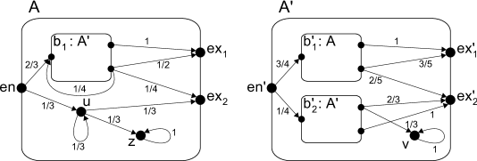
A Recursive Markov Chain (RMC) consists of components, which are analogous to procedure definitions in a procedural language. The structure of each component is similar to an automaton, with the addition of boxes that represent procedure calls. An RMC can be considered as an extension of DTMCs with recursively-called components. An example RMC from [7] is shown in Fig. 6. There are four special node types in an RMC: entry ($en$) and exit nodes ($ex$) associated with components and call and return ports associated with boxes. In a box, call and return ports correspond to entry and exit nodes, respectively, of the called component. Behaviors of an RMC are the set of runs with matching calls and returns. Hence behaviors of an RMC form a context free language. We pose the problem of reachability in an RMC (i.e. the probability of the set of runs that hit a given state) in terms of GPL model checking of a corresponding RPLTS.

Figure 7: RPLTS corresponding to the example RMC in Fig. 6

Given an RMC $R$, in which the maximum number of exits in any component is $n$, we define an RPLTS $R^{\prime}$ and a set of $n$ mutually recursive GPL formulae $X_{1},X_{2},\ldots,X_{n}$. $R^{\prime}$ will have a state for every node of $R$, in particular including the call and return ports of each box. For each probabilistic transition in $R$, we add the same transition in $R^{\prime}$ and label it as $p$. To model the recursive call, we introduce three types of transitions. From the state $s$ in $R^{\prime}$ corresponding to a call port in $R$, we add a $c$ (call) transition to state $s^{\prime}$ corresponding to the called component’s entry node. We also add $r_{i}$ (return) transitions from state $s$ to the states corresponding to the return ports of the call. Finally, from state $s$ in $R^{\prime}$ corresponding to an exit node $\mbox{\it ex\/}_{i}$, we add an $e_{i}$ (exit) transition back to $s$. The exit transitions and their labels enable us to write GPL formulae that check for termination. The RPLTS corresponding to the example RMC in Fig. 6 is shown in Fig. 7. Labels on probabilistic transitions ($p$) are omitted in Fig. 7 to avoid clutter.

We use GPL formulae $X_{i}$ to specify behaviors in an RMC that eventually reach an exit node $\mbox{\it ex\/}_{i}$ of a component. For a 2-exit RMC, the definitions of $X_{i}$ are as follows:

$$\mbox{\tt def}(X_{1},\mbox{\tt lfp}(\mbox{\tt or}( \mbox{\tt diam}(e_{1},\mbox{\tt tt}),$$

$$\mbox{\tt or}( \mbox{\tt diam}(p,X_{1}),$$

$$\mbox{\tt or}( \mbox{\tt and}(\mbox{\tt diam}(c,X_{1}),\mbox{\tt diam}(r_{1},X_{1})),$$

$$\mbox{\tt and}(\mbox{\tt diam}(c,X_{2}),\mbox{\tt diam}(r_{2},X_{1}))))))).$$

$$\mbox{\tt def}(X_{2},\mbox{\tt lfp}(\mbox{\tt or}( \mbox{\tt diam}(e_{2},\mbox{\tt tt}),$$

$$\mbox{\tt or}( \mbox{\tt diam}(p,X_{2}),$$

$$\mbox{\tt or}( \mbox{\tt and}(\mbox{\tt diam}(c,X_{1}),\mbox{\tt diam}(r_{1},X_{2})),$$

$$\mbox{\tt and}(\mbox{\tt diam}(c,X_{2}),\mbox{\tt diam}(r_{2},X_{2}))))))).$$

The intuition behind the formulae for $X_{i}$ is as follows. Since $X_{i}$ specifies that $\mbox{\it ex\/}_{i}$ is eventually reached, $X_{i}$ is a least fixed point formula. The ways in which exit $\mbox{\it ex\/}_{i}$ is reached from a state $s$ are:

1. $e_{i}$ transition is enabled at $s$: this corresponds to the disjunct $\mbox{\tt diam}(e_{i},\mbox{\tt tt})$ in the definition of $X_{i}$;

2. there is a probabilistic transition ($p$) from $s$ to $s^{\prime}$ such that $\mbox{\it ex\/}_{i}$ is reached eventually from $s^{\prime}$ (corresponds to ($\mbox{\tt diam}(p,X_{i})$);

3. $s$ corresponds to a call, that call eventually returns from $\mbox{\it ex\/}_{j}$ for some $j$, and subsequently, $\mbox{\it ex\/}_{i}$ is reached. The formula $\mbox{\tt and}(\mbox{\tt diam}(c,X_{j}),\mbox{\tt diam}(r_{j},X_{i}))$ encodes this way of reaching $\mbox{\it ex\/}_{i}$ via $\mbox{\it ex\/}_{j}$. The subformula $\mbox{\tt diam}(c,X_{j})$ specifies that $\mbox{\it ex\/}_{j}$ is reached after the call; and the subformula $\mbox{\tt diam}(r_{j},X_{i})$ specifies that after the corresponding return, $\mbox{\it ex\/}_{i}$ is eventually reached.

While the example shows the GPL formulae for 2-exit RMCs, the description above gives the general structure of the formulae for $n$-exit RMCs. Note that if a component has fewer than $n$ exits, then the formula $X_{n}$ will be trivially false at all of its nodes. Moreover, behaviors satisfying $X_{i}$ and those satisfying $X_{j}$ ($i\not=j$) are mutually exclusive, since we cannot terminate at more than one exit on a single path. Finally, the GPL formula is the same regardless of what RMC we are attempting to transform, and only depends on $n$.

6 Experimental Results

PIP has been implemented using the XSB tabled logic programming system [42]. An explanation generator is constructed by performing normal query evaluation under the well-founded semantics by redefining msws to backtrack through their potential values, and have the undefined truth value. This generates a residual program in XSB that captures the dependencies between the original goal and the msws (now treated as undefined values). In one partial implementation, called PIP-Prism, the probabilities are computed directly from the residual program. Note that such a computation will be correct if PRISM’s restrictions are satisfied. In general, however, we materialize the residual program into a dynamic database that corresponds to the productions in the explanation generator. A second partial implementation, called PIP-BDD, constructs BDDs from the explanation generator, and computes probabilities from the BDD. Note that PIP-BDD will be correct when the finiteness restriction holds. The full implementation of PIP, called PIP-full, is obtained by constructing a set of FEDs from the explanation generator (Def. 8), generating polynomial equations from the set of FEDs (Def. 11) and finally finding the least solution to the set of equations. The final equation solver is implemented in C. All other parts of the three implementations, including the BDD and FED structures, are completely implemented in tabled Prolog.

We present two sets of experimental results, evaluating the performance of PIP on (1) programs satisfying PRISM’s restrictions; and (2) a program for model checking PCTL formulae.

Performance on PRISM Programs:

Note that all three implementations— PIP-Prism, PIP-BDD and PIP-full may be used to evaluate PRISM programs.

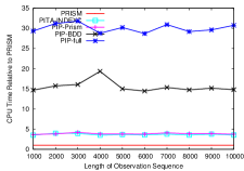
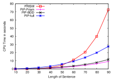
(a) Relative performance on HMM	(b) Performance for NCN queries for PLC
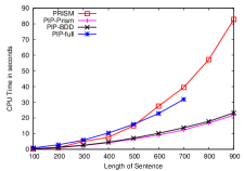
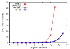
(c) Performance for NPV queries for PLC	(d) Performance for ADVN queries for PLC

Figure 8: Performance of PIP on PRISM Programs

Hidden Markov Model (HMM):

We used the simple 2-state gene sequence HMM from [2] (also used in [37]) for our evaluation. We measured the CPU time taken by the versions of PIP, PRISM 2.0.3 and PITA-INDEXC [37] (a version of PITA that does not use BDDs and uses PRISM’s assumption) to evaluate the probability of a given observation sequence, for varying sequence lengths. The observation sequence itself was embedded as a set of facts (instead of an argument list). This makes table accesses fast even when shallow indices are used. The performance of the three PIP versions and PITA-INDEXC, relative to PRISM 2.0.3, is shown in Fig. 8(a). CPU times are normalized using PRISM’s time as the baseline. Observe that the PIP-Prism and PITA-INDEXC perform similarly: about 3.5 to 4 times slower than PRISM. Construction of BDDs (done in PIP-BDD, but not in PIP-Prism) adds an extra factor of 4 overhead. Construction of full-fledged FEDs, generating polynomial equations and solving them (done only in PIP-full) adds another factor of 2 overhead. We find that the equation-solving time (using the only component coded in C) is generally negligible.

Probabilistic Left Corner Parsing:

This example was adapted from PRISM’s example suite, parameterizing the length of the input sequence to be parsed. We measured the CPU time taken by the three versions of PIP and PRISM 2.0.3 on a machine with an Intel Pentium 2.16GHz processor. The performance on three queries (each encoding a different class of strings) is shown in Fig. 8(b)–(d). In contrast to the HMM example, the sequences are represented as lists. For these examples, PIP-Prism implementation outperforms PRISM. Moreover, although PIP-BDD and PIP-full are slower than PIP-Prism, the relative performance gap is much smaller than observed in the HMM example.

(a) $N=5$	(b) $N=6$

Figure 9: Performace of PCTL model checking using PIP and the Prism model checker for Synchronous Leader Election protocol of different sizes

Performance of the PCTL Model Checker:

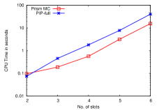
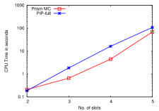
We evaluated the performance of PIP-full for supporting a PCTL model checker (encoded as shown in Fig. 4). We compared the performance of PIP-based model checker with that of the widely-used Prism model checker [22]. We show the performance of PIP and the Prism model checker on the Synchronous Leader Election Protocol [17] for computing the probability that eventually a leader will be elected. Fig. 9 shows the CPU time used to compute the probabilities of this property on systems of different sizes. Observe that our high-level implementation of a model checker based on PIP performs within a factor of 3 of the Prism model checker (note: the y-axis on these graphs is logarithmic). Moreover, the two model checkers show similar performance trends with increasing problem instances. However, it should be noted that the Prism model checker uses a BDD-based representation of reachable states, which can, in principle, scale better to large state spaces compared to the explicit state representation used in our PIP-based model checker.

7 Conclusions

In this paper, we have shown that in order to formulate the problem of probabilistic model checking in probabilistic logic programming, one needs an inference algorithm that functions correctly even when finiteness, mutual-exclusion, and independence assumptions are simultaneously violated. We have presented such an inference algorithm, PIP, implemented it in XSB Prolog, and demonstrated its practical utility by using it as the basis for encoding model checkers for a rich class of probabilistic models and temporal logics.

For future work, we plan to refine and strengthen the implementation of PIP. We also plan to explore more substantial model-checking case studies. It would be interesting to study whether optimizations to exploit data independence and symmetry, which are easily enabled by high-level encodings of model checkers, will be effective for probabilistic systems as well.

Acknowledgments.

Research supported in part by NSF Grants CCF-1018459 CCF-0926190, CCF-0831298, AFOSR Grant FA9550-09-1-0481, and ONR Grant N00014-07-1-0928.

References

- [1] C. Baier. On Algorithmic Verification Methods for Probabilistic Systems. Habilitation thesis, Fakultät für Mathematik & Informatik, Universität Mannheim, 1998.
- [2] H. Christiansen and J. P. Gallagher. Non-discriminating arguments and their uses. In ICLP, volume 5649 of LNCS, pages 55––69, 2009.
- [3] R. Cleaveland, S. P. Iyer, and M. Narasimha. Probabilistic temporal logics via the modal mu-calculus. Theor. Comput. Sci., 342(2-3):316–350, 2005.
- [4] L. De Raedt, A. Kimmig, and H. Toivonen. ProbLog: A probabilistic Prolog and its application in link discovery. In IJCAI, pages 2462–2467, 2007.
- [5] G. Delzanno and A. Podelski. Model checking in CLP. In TACAS, pages 223–239, 1999.
- [6] X. Du, C. R. Ramakrishnan, and S. A. Smolka. Tabled resolution + constraints: A recipe for model checking real-time systems. In IEEE Real Time Systems Symposium (RTSS), 2000.
- [7] K. Etessami and M. Yannakakis. Recursive Markov chains, stochastic grammars, and monotone systems of nonlinear equations. J. ACM, 56(1), 2009.
- [8] B. Farwer and M. Leuschel. Model checking object Petri nets in Prolog. In PPDP, pages 20–31, 2004.
- [9] N. Friedman, L. Getoor, D. Koller, and A. Pfeffer. Learning probabilistic relational models. In IJCAI, pages 1300–1309, 1999.
- [10] L. Getoor and B. Taskar. Introduction to Statistical Relational Learning. The MIT Press, 2007.
- [11] G. Gupta, A. Bansal, R. Min, L. Simon, and A. Mallya. Coinductive logic programming and its applications. In ICLP, pages 27–44, 2007.
- [12] G. Gupta and E. Pontelli. A constraint based approach for specification and verification of real-time systems. In Proceedings of the Real-Time Systems Symposium, 1997.
- [13] B. Gutmann, M. Jaeger, and L. D. Raedt. Extending ProbLog with continuous distributions. In Proceedings of ILP, 2010.
- [14] B. Gutmann, I. Thon, A. Kimmig, M. Bruynooghe, and L. D. Raedt. The magic of logical inference in probabilistic programming. TPLP, 11(4–5):663–680, 2011.
- [15] H. Hansson and B. Jonsson. A Logic for Reasoning about Time and Reliability. Formal Aspects of Computing, 6(5):512–535, 1994.
- [16] M. A. Islam, C. R. Ramakrishnan, and I. V. Ramakrishnan. Inference in Probabilistic Logic Programs with Continuous Random Variables. ArXiv e-prints, Dec. 2011. http://arxiv.org/abs/1112.2681.
- [17] A. Itai and M. Rodeh. Symmetry breaking in distributive networks. In FOCS, pages 150–158, 1981.
- [18] K. Kersting and L. D. Raedt. Bayesian logic programs. In ILP Work-in-progress reports, 2000.
- [19] K. Kersting and L. D. Raedt. Adaptive Bayesian logic programs. In Proceedings of ILP, 2001.
- [20] D. Kozen. Results on the propositional -calculus. Theoretical Computer Science, 27:333–354, 1983.
- [21] A. Kucera, J. Esparza, and R. Mayr. Model checking probabilistic pushdown automata. Logical Methods in Computer Science, 2(1), 2006.
- [22] M. Kwiatkowska, G. Norman, and D. Parker. PRISM 4.0: Verification of probabilistic real-time systems. In Proc. 23rd International Conference on Computer Aided Verification (CAV’11), volume 6806 of LNCS, pages 585–591. Springer, 2011.
- [23] R. Milner. Communication and Concurrency. International Series in Computer Science. Prentice Hall, 1989.
- [24] R. Milner, J. Parrow, and D. Walker. A calculus of mobile processes, Parts I and II. Information and Computation, 100(1):1–77, 1992.
- [25] S. Muggleton. Stochastic logic programs. In Advances in inductive logic programming, 1996.
- [26] S. Mukhopadhyay and A. Podelski. Beyond region graphs: Symbolic forward analysis of timed automata. In FSTTCS, pages 232–244, 1999.
- [27] S. Mukhopadhyay and A. Podelski. Model checking for timed logic processes. In Computational Logic, pages 598–612, 2000.
- [28] P. Narman, M. Buschle, J. Konig, and P. Johnson. Hybrid probabilistic relational models for system quality analysis. In Proceedings of EDOC, 2010.
- [29] G. Pemmasani, C. R. Ramakrishnan, and I. V. Ramakrishnan. Efficient model checking of real time systems using tabled logic programming and constraints. In International Conference on Logic Programming (ICLP), LNCS. Springer, 2002.
- [30] D. Poole. The independent choice logic and beyond. In Probabilistic ILP, pages 222–243, 2008.
- [31] Y. S. Ramakrishna, C. R. Ramakrishnan, I. V. Ramakrishnan, S. A. Smolka, T. Swift, and D. S. Warren. Efficient model checking using tabled resolution. In CAV, volume 1254 of LNCS, pages 143–154. Springer, 1997.
- [32] C. R. Ramakrishnan. A model checker for value-passing mu-calculus using logic programming. In Practical Aspects of Declarative Languages (PADL), volume 1990 of LNCS, pages 1–13. Springer, 2001.
- [33] C. R. Ramakrishnan et al. XMC: A logic-programming-based verification toolset. In CAV, number 1855 in LNCS, pages 576–580, 2000.
- [34] M. Richardson and P. Domingos. Markov logic networks. Machine Learning, 2006.
- [35] F. Riguzzi and T. Swift. An extended semantics for logic programs with annotated disjunctions and its efficient implementation. In Italian Conference on Computational Logic, volume 598 of CEUR Workshop Proceedings, 2010.
- [36] F. Riguzzi and T. Swift. Tabling and answer subsumption for reasoning on logic programs with annotated disjunctions. In Technical Communications of the International Conference on Logic Programming, pages 162––171, 2010.
- [37] F. Riguzzi and T. Swift. The PITA system: Tabling and answer subsumption for reasoning under uncertainty. TPLP, 11(4–5):433–449, 2011.
- [38] V. Santos Costa, D. Page, M. Qazi, and J. Cussens. CLP(): Constraint logic programming for probabilistic knowledge. In Proceedings of the 19th Conference on Uncertainty in Artificial Intelligence (UAI03), pages 517–524, Acapulco, Mexico, August 2003.
- [39] B. Sarna-Starosta and C. R. Ramakrishnan. Constraint-based model checking of data-independent systems. In International Conference on Formal Engineering Methods (ICFEM), volume 2885 of Lecture Notes in Computer Science, pages 579–598. Springer, 2003.
- [40] T. Sato and Y. Kameya. PRISM: a symbolic-statistical modeling language. In IJCAI, 1997.
- [41] A. Singh, C. R. Ramakrishnan, and S. A. Smolka. A process calculus for mobile ad hoc networks. In 10th International Conference on Coordination Models and Languages (COORDINATION), volume 5052 of LNCS, pages 296–314. Springer, 2008.
- [42] T. Swift, D. S. Warren, et al. The XSB logic programming system, Version 3.3, 2012. http://xsb.sourceforge.net.
- [43] J. Vennekens, M. Denecker, and M. Bruynooghe. CP-logic: A language of causal probabilistic events and its relation to logic programming. TPLP, 2009.
- [44] J. Vennekens, S. Verbaeten, and M. Bruynooghe. Logic programs with annotated disjunctions. In ICLP, pages 431–445, 2004.
- [45] J. Wang and P. Domingos. Hybrid Markov logic networks. In Proceedings of AAAI, 2008.
- [46] D. Wojtczak and K. Etessami. PReMo: an analyzer for probabilistic recursive models. In TACAS, 2007.
- [47] P. Yang, C. R. Ramakrishnan, and S. A. Smolka. A logical encoding of the pi-calculus: Model checking mobile processes using tabled resolution. International Journal on Software Tools for Technology Transfer (STTT), 6(1):38–66, 2004.