Interplay between Kondo tunneling and Rashba precession

Abstract

The influence of Thomas – Rashba precession on the physics of Kondo tunneling through quantum dots is analyzed. It is shown that this precession is relevant only at finite magnetic fields. Thomas – Rashba precession results in peculiar anisotropy of the effective g-factor and initiates dephasing of the Kondo tunneling amplitude at low temperature, that is strongly dependent on the magnetic field.

I Introduction

Spin precession due to Rashba coupling Raby in a 2D electron gas (2DEG) is a specific manifestation of the fundamental Thomas effect of spin precession in magnetic component of electromagnetic field due to spin-orbit interaction. This relativistic effect is strongly enhanced in semiconductors, and in particular in 2DEG in semiconductor heterostructures.Rashba A necessary precondition for the occurrence of Thomas – Rashba (TR) precession in semiconductors is an asymmetry of confinement potential characterized by a vector $\vec{n}$ pointing along the electric field. An interesting physical situation may show up when the TR precession is noticeable in 2DEG in which magnetic impurities are immersed. Since electron scattering by magnetic impurities results in the Kondo effect, a natural question is whether and how the Kondo scattering is sensitive to the TR spin precession. Prima facie it seems that this precession is irrelevant to the physics of Kondo screening. In the presence of spin orbit coupling, the degenerate two level system is composed of spiral states (Kramers pair), determined by the spirality winding number (and not by the spin projection quantum number as in systems respecting spin rotation invariance). But this distinction simply leads to re-scaling of the Kondo model’s parameters without affecting the Kondo physics. This direct reasoning is supported by basic argumentsMewin stating that, due to time-reversal symmetry, spin-orbit scattering does not suppress the Kondo effect even though it breaks spin-rotation invariance. Subsequent investigationsKavo ; Malec confirmed this conclusion. At finite external magnetic field, time reversal invariance is broken, and additional mechanisms affecting Kondo tunneling arises together with the conventional Zeeman splitting of the impurity levels, as was demonstrated in Ref. Mewin, for the case of dirty metals.

On the other hand, it has been arguedZar that an admixture of nonzero angular modes of spiral states in a 2DEG with TR precession Malec might cause an enhancement of the Kondo temperature due to renormalization of the effective exchange integral. Similar arguments apply for non-centrosymmetruc cubic crystalsAgt . A special case of Kondo effect in the presence of local Rashba coupling in quantum wires has recently been considered, where it is shownSerSan06 ; SerSan07 ; Xu that Rashba effect may be the source of resonant states in the bands and thereby induce the Kondo effect. Thus, there are cases where Rashba-type spin-orbit coupling affects the Kondo physics. In that sense we may refer to it as Kondo-Rashba effect.

In the present paper we discuss the physical content of the interplay between the TR precession and the Kondo effect inherent in quantum dots under the constraint of strong Coulomb blockade.Kougla The source of this interlacing may be due both to the sizable Rashba-type spin-orbit coupling in the leads and the TR precession in the complex ring-like geometry of the dots.Bergsten ; Koenig ; Aono We stress the specific features of Kondo-Rashba effect in quantum dot devices in comparison with that resulting from magnetic impurities immersed in 2DEG.Mewin ; Malec As already noted above, the TR precession is relevant for Kondo tunneling only under an external magnetic field. We show here that this relevance stems from the fact that the spin coordinate axes tilt due to the TR precession. The tilting axes for the dot and the leads are distinct, and it is not possible to match two reference frames in the presence of an external magnetic field. As a result of the TR effect, the Kondo scattering becomes fully anisotropic, and this anisotropy is relevant for the screening mechanism. In addition, the spatial separation of the Kondo impurity (the localized electron at the dot) and the leads result in non-local indirect exchange, and this non-locality is explicitly related to the TR contribution to the indirect exchange.

Unremovable mismatch of local magnetic axes is a salient feature of Dzyaloshinskii-Moriya exchange in some low-symmetry magnetic crystals.Mory It will be shown that the indirect exchange between spins in the dot and in the leads mediated by Rashba coupling has the same vector structure as the Dzyaloshinskii-Moriya interaction between adjacent localized spins. The relevance TR effect to indirect exchange has been perceived in previous studies. In particular, the Ruderman-Kittel-Kasuya-Yoshida (RKKY) interaction between localized spins in 2DEG with Rashba type spin-orbit coupling is characterized by the above mentioned mismatch of local magnetic axes.Kavo ; Imam ; Simon . Similar mismatch occurs in devices consisting of QD with Rashba interaction in contact with two ferromagnetic leadsSun and in system consisting of two magnetic impurities in a ring pierced by electric and magnetic fieldsAono .

II Kondo-Rashba coupling in external magnetic field

Within the analysis of Kondo effect in quantum dot with fixed (odd) number of electrons in weak tunneling contact with source and drain leads, the starting point is an effective spin Hamiltonian supplemented by TR term,

$$H = \varepsilon_{d}\sum_{\sigma}n_{d\sigma}+\frac{U}{2}\sum_{\sigma}n_{d\sigma}n_{d\bar{\sigma}}+\sum_{k\sigma}\varepsilon_{k}n_{k\sigma}$$ (1)

$$+ H_{\rm cot}+H_{{\mbox{\tiny TR}}}.$$

The first two terms encode the quantum dot, with electron operators $d_{\sigma},d^{\dagger}_{\sigma}$, number operator $n_{d\sigma}=d^{\dagger}_{\sigma}d_{\sigma}$, discrete electron level $\varepsilon_{d}$ and Coulomb blockade energy $U$. The continuum (band) states in the leads are characterized by energies $\varepsilon_{k}$ and number operators $n_{k\sigma}=c^{\dagger}_{k\sigma}c_{k\sigma}$. Assuming the left ($l$) and right ($r$) leads to be identical, only the even combination $c_{k\sigma}=(c_{lk\sigma}+c_{rk\sigma})/\sqrt{2}$ survives in the effective Hamiltonian. The next term, $H_{\rm cot}$, represents an effective cotunneling resulting from the Schrieffer-Wolff (SW) transformation applied on the original Anderson Hamiltonian. The last term in (1) stands for the TR precession.

In order to expose the key features of the interplay between TR precession and Kondo tunneling and to elucidate the triggering role of magnetic field, we first adopt a phenomenological approach. Consider a model where both the leads and the dot are subject to TR precession. Each subsystem $i=l$ (for lead), $d$ (for dot) is characterized by its own TR coupling with a Rashba vector $\vec{n}_{i}$ and coupling strength $\vec{w}_{i}$. (The microscopic substantiation for this model will be presented at the end of this section). The effective spin Hamiltonian $H_{\rm s}$ for the lead-dot device in an external magnetic field $\vec{H}$ (entering through the the Zeeman Hamiltonian $H_{\mbox{\tiny Z}}$) has the form

$$H_{\rm s}=H_{{\mbox{\tiny TR}}}+H_{{\mbox{\tiny Z}}}+H_{\rm cot}=$$ (2)

$$\vec{n}_{d}\cdot(\vec{S}\times\vec{w}_{d})+\vec{n}_{l}\cdot(\vec{\sigma}\times\vec{w}_{l})+{\vec{h}}_{d}\cdot{\vec{S}}+{\vec{h}}_{l}\cdot{\vec{\sigma}}+J\vec{S}\cdot\vec{\sigma}.$$

Here $\vec{S}$ is the dot electron spin 1/2 operator, $\vec{\sigma}=\sum_{kk^{\prime}}\sum_{\sigma\sigma^{\prime}}c^{{\dagger}}_{k\sigma}\vec{\tau}c_{k^{\prime}\sigma^{\prime}}$ is the lead spin 1/2 conduction electrons operator, $\vec{\tau}$ is the vector of Pauli matrices and ${\vec{h}}_{i}=g_{i}\mu_{{\mbox{\tiny B}}}{\vec{H}}$. The TR coupling is given by $\vec{w}_{i}=\alpha_{i}\vec{p}_{i}$, where $\alpha_{i}$ and $\vec{p}_{i}$ are TR coupling constants and momentum operators for dot and lead subsystems. External magnetic field $\vec{H}$ fixes the direction of the original $z$ axis of spin coordinate system, but the vectors $\vec{w}_{d},~{}\vec{w}_{l}$ in general case are not parallel and have different moduli. In many cases the factors $g_{i}$ are also different in magnitude and sometimes they even have opposite signs, so we retain the index $i$ in the Zeeman terms as well.

It is seen from Eq. (2), that the spin precession described by $H_{\mbox{\tiny TR}}$ results in rotation of spin axes established by the Zeeman term $H_{\mbox{\tiny Z}}$, but the rotation angles are different for dot and lead subsystems,

$$\vec{S}^{\prime}={\sf T}(\Theta_{d},\Phi_{d})\vec{S},~{}~{}~{}\vec{\sigma}^{\prime}={\sf T}(\Theta_{l},\Phi_{l})\vec{\sigma},$$ (3)

where ${\sf T}(\Theta,\Phi)$ is an appropriate rotation matrix (see below). In the simplest case where both Rashba vectors are parallel to the $z$-axis but the coupling constants are different in magnitude, $\vec{n}_{i}=(0,0,1)$, $\vec{w}_{i}=(w_{ix},w_{iy},0)$, the dot Hamiltonian

$$H_{\mbox{\tiny Z}}+H_{\mbox{\tiny TR}}=h_{dz}S_{z}+(h_{dx}+w_{dy})S_{x}+(h_{dy}-w_{dx})S_{y}~{}.$$ (4)

is transformed to a new spin frame by means of the rotation matrix,

$${\sf T}(\Theta_{d},\Phi_{d})=$$ (9)

$$\left(\begin{array}[]{ccc}\cos\Theta_{d}\cos\Phi_{d}&-\cos\Theta_{d}\sin\Phi_{d}&\sin\Theta_{d}\\ \sin\Phi_{d}&\cos\Phi_{d}&0\\ -\sin\Theta_{d}\cos\Phi_{d}&\sin\Theta_{d}\sin\Phi_{d}&\cos\Theta_{d}\end{array}\right)$$

The Euler angles are given by the equations

$$\tan\Theta_{d}=\frac{|w_{d}|}{h_{dz}},~{}~{}~{}\tan\Phi_{d}=\frac{w_{dy}+h_{dx}}{w_{dx}-h_{dy}}.$$ (10)

Thus, the quantities $w^{2}_{d\perp}=w_{dx}^{2}+w_{dy}^{2}$ and $h^{2}_{d\perp}=h_{dx}^{2}+h_{dy}^{2}$ define the modulus of a planar component of an effective magnetic field $\Delta_{\perp}^{2}=w_{d\perp}^{2}+h_{d\perp}^{2}$. Similar transformation for the Hamiltonian $H_{\mbox{\tiny Z}}^{(l)}+H^{(l)}_{\mbox{\tiny TR}}$ yields analogous equations to (10) for the Euler angles $(\Theta_{l},\Phi_{l})$, with $w_{l},h_{l}$ substituted for $w_{d},h_{d}$.

If the system preserves the square symmetry, then $\Phi_{d}=\Phi_{l}=\pi/4$, but $\Theta_{d}\neq\Theta_{l}$ unless $\vec{H}=0$. In the latter case $\Theta_{d}=\Theta_{l}=\pi/2$, and the rotation of spin coordinates is the same for both subsystems. Fig. 1 illustrates this rotation.

Figure 1: Rotation of spin axes induced at $\vec{H}=0$ by $H_{\mbox{\tiny TR}}$. The two Euler angles are $\Theta=\pi/2$, $\Phi=\pi/4$. Intermediate and final coordinates are indicated by primes and double primes, respectively. Initial, intermediate and final coordinates are shown by solid, dashed and bold dashed lines, respectively.

It follows from (3) that, after rotation operation, the cotunneling part of the spin Hamiltonian (2) acquires the form

$$H_{\rm cot}={\widetilde{J}}\vec{S}^{\prime}(\Omega_{d})\cdot\vec{\sigma}^{\prime}(\Omega_{l}),$$ (11)

(cf. Refs. Imam, ; Sun, ; Aono, ). Here $\Omega_{d(l)}=\{\Theta_{d(l)},\Phi_{d(l)}\}$. Thus we conclude that the unified spin coordinate system for the dot and the leads shown in Fig. 1 may be established only in zero magnetic field $\vec{H}=0$. Otherwise, one deals with anisotropic Kondo tunneling, and this anisotropy is relevant when $\vec{H}\neq 0$.Affl

The indirect exchange Hamiltonian (11) may be reduced to the familiar Dzyaloshinskii-Moriya form in case of strong magnetic field $h_{iz}\gg w_{i}$. In this case the angle $\Theta_{i}\ll\pi/2$,, so that $\sin\Theta_{i}\approx w_{i}/h_{iz},~{}\cos\Theta_{i}\approx 1$. On the other hand, the difference between $\Phi_{d}$ and $\Phi_{l}$ can be substantial, especially when the planar magnetic field $h_{i\perp}$ is comparable with $w_{i}$. In this case the axes $m_{dz},m_{lz}$ of the spin reference frames for $\vec{S}^{\prime}$ and $\vec{\sigma}^{\prime}$ are nearly parallel, whereas the divergence between the in-plane projections $\{m_{dx},m_{dy}\}$ and $\{m_{lx},m_{ly}\}$ may be noticeable. One may then choose the frame $\texttt{M}_{l}=\{m_{lx},m_{ly},m_{lz}\}$ connected with the leads as the common reference frame for spins $\vec{S}$ and $\vec{\sigma}$ and then expand the rotated spin $\vec{S}^{\prime}$ (3) around the spin $\vec{S}$ determined in the frame M_l. Neglecting the small difference of the projections along $z$, the tilt $\phi$ of the dot spin can be presented by the vector equality

$$\vec{S}^{\prime}=\vec{S}+\phi\ (\vec{n}_{l}\times\vec{S}),$$ (12)

(see Fig. 2). Here we used the fact that the Rashba vector $\vec{n}_{l}$ coincides with $m_{lz}$).

Figure 2: Spin rotation in the presence of the Rashba vector $\vec{n}$ directed along $\hat{\bf z}$. $m_{x},m_{y}$ are the components of the unit vector in the $(x-y)$ plane.

The angle $\phi\sim\Phi_{d}-\Phi_{l}$ is assumed to be small. Otherwise, a more general expression

$$\vec{S}^{\prime}=\vec{S}+\sin\phi((\vec{n}\times\vec{S}))+\cos\phi(\vec{S}-\vec{n}(\vec{n}\cdot\vec{S}))$$ (13)

should be used instead of (12).

Substituting Eq. (12) into (11), we arrive at the effective cotunneling Hamiltonian expressed in the reference frame M_l related to the leads

$$H_{\rm cot}=J{\vec{S}}\cdot{\vec{\sigma}}+{\vec{j}}(\vec{S}\times{\vec{\sigma}})$$ (14)

where ${\vec{j}}=J\phi\vec{n}$ is the TR induced anisotropic component of the exchange coupling constant.

A microscopic substantiation of the phenomenological assumption (3) should now be presented. The TR precession in 2DEG is presented by continuous set of vectors ${\vec{w}}_{l}(\vec{k})=\alpha\vec{k}$, where $\vec{k}$ is the wave vector in the 2D Brillouin zone.Malec To reduce this continuum to a single vector, one should explicitly take into account the spatial non-locality of the lead-dot indirect exchange induced by cotunneling processes.

In realistic devices, the TR coupling exists in the planar leads, and there is no generic spin-orbit interaction in the dot. Then the lead continuum is encoded in Kondo tunneling through the properties of the band electrons in the point ${\vec{R}}$, which denotes the ”entrance” coordinate of the tunneling channel relative to the dot spin position (located at at $\vec{R}=0$). Taking into account the non-locality of electron cotunneling, one should write the effective spin Hamiltonian obtained by means of the SW transformation in the form

$$H_{\rm cot}=J\vec{S}\cdot{\vec{\sigma}}_{\vec{R}}$$ (15)

where ${\vec{\sigma}}_{\vec{R}}=\sum_{{{\vec{k}}{\vec{k}}^{\prime}}}\sum_{\sigma\sigma^{\prime}}c^{{\dagger}}_{{\vec{k}}\sigma}\vec{\tau}c_{{\vec{k}}^{\prime}\sigma^{\prime}}\exp[{i({\vec{k}}-{\vec{k}}^{\prime}){\vec{R}}}]$. Then the TR field is presented by its local component in the point $\vec{R}$ (see, e.g., Ref. Imam, )

$$H_{\mbox{\tiny TR}}^{loc}=\alpha_{l}({\vec{\sigma}}\times\hat{r})F(R).$$ (16)

Here $\hat{r}=\vec{R}/R$ is a unit vector along $\vec{r}$ and $F(R)$ is the form factor arising within the procedure of Fourier transformation. This means that the planar TR components of the effective magnetic field in the leads are the components of the vector ${\vec{w}_{l}}=\alpha F(R)\hat{r}$.

Another system where the conjecture expressed in Eq. (3) is realized consists of a quantum dot possessing TR coupling term, whereas the spin-orbit interaction in the leads is negligible. This regime may be realized, e.g., in transition metal-organic complex adsorbed on a metallic substrate in contact with a nano-tip of a tunneling microscope. In this type of devices the source of the TR term is the asymmetry of the electric field induced by the nano-tip. Then it is natural to choose the frame for the leads with the axis $\sigma_{z}\parallel h_{z}$ and two other axes oriented in such a way that the system of coordinates $\texttt{M}_{d}\{m_{dx},m_{dy},m_{dz}\}$ is only slightly tilted relative to the reference frame. Then one may adjust the two coordinate systems by means of the vector equality

$$\vec{S}^{\prime}=\vec{S}+\phi((\vec{n}_{d}\times\vec{S}))$$ (17)

like in Eq. (12) and thereby arrive at the same anisotropic spin Hamiltonian (14), which describes the interplay between TR and Kondo mechanisms.

III Scaling analysis of anisotropic Thomas-Rashba-Kondo Hamiltonian

Based on the above analysis, we now study the interplay between the TR precession and the Kondo effect in the weak coupling regime $T\gg T_{K}$, where the RG scaling approach for identifying the fixed points is applicable. In the two limiting cases of strong and weak magnetic field, the general Hamiltonian (11) is reducible to a simplified effective Hamiltonian (14), as discussed below.

III.1 Strong magnetic field

Following our analysis of the previous section, the anisotropic Thomas-Rashba-Kondo Hamiltonian reads,

$$H=\sum_{k\sigma}\varepsilon_{k}n_{k\sigma}+\vec{h}_{d}\cdot\vec{S}+J{\vec{S}}\cdot{\vec{\sigma}}+{\vec{j}}(\vec{S}\times{\vec{\sigma}}).$$ (18)

This form entails a Rashba vector that is parallel to the $z$-axis and a strong external magnetic field $\vec{H}\parallel\hat{\bf z}$, so that $\vec{h}_{d}=\{w_{dx},w_{dy},h\}$ and $h\gg w_{d}$. The second term is the spin Hamiltonian of the isolated dot

$$H_{{\mbox{\tiny Z}}}+H_{\mbox{\tiny TR}}=h_{z}S_{z}+\frac{1}{2}\left(w_{d}S^{+}+w_{d}^{*}S^{-}\right)~{},$$ (19)

where $w_{d}=w_{dy}+iw_{dx}$. The last two terms in Eq. (18) form the co-tunneling part, rewritten as,

$$H_{{\mbox{\tiny cot}}}=\frac{1}{2}\left(J_{-}\sigma_{+}S_{-}+J_{+}\sigma_{-}S_{+}\right)+J\sigma_{z}S_{z},$$ (20)

with

$$J_{\pm}=J(1\pm i\phi),$$ (21)

and $\phi\approx|w_{d}|/h$. Thus, the spin-related part of the above Hamiltonian is generically anisotropic. To expose the evolution (flow) of the anisotropy parameters we define

$$J_{+}-J_{-}=2iJ\phi\equiv 2ij_{\mbox{\tiny TR}}~{},$$ (22)

where $j_{\mbox{\tiny TR}}=J\phi_{d}$ is the modulus of the Kondo – Rashba vector coupling in the Hamiltonian (18). It is readily seen from Eq. (22) that the magnetic anisotropy induced by TR precession increases on approaching the standard infinite fixed point and hence it is relevant.

In the weak coupling limit one may study the Kondo problem using ”poor man’s scaling” perturbative approach.Andrg In our case with TR term present, deviation from the standard scaling paradigm arises already in zero order in the exchange constant because the Kondo problem should be solved in the presence of an effective ”magnetic” field given by Eq. (19). Using the pseudofermion representation for spin operator $\vec{S}=\sum_{\sigma\sigma^{\prime}}f^{\dagger}_{\sigma}\vec{\tau}f_{\sigma^{\prime}}$, we rewrite (19) as

$$H_{{\mbox{\tiny TR}}}+H_{{\mbox{\tiny Z}}}=\frac{h}{2}(f^{\dagger}_{\uparrow}f_{\uparrow}-f^{\dagger}_{\downarrow}f_{\downarrow})+\frac{1}{2}\left(w_{d}f^{{\dagger}}_{\uparrow}f_{\downarrow}+w_{d}^{*}f^{{\dagger}}_{\downarrow}f_{\uparrow}\right)$$ (23)

In accordance with the arguments adduced in the previous section, this ”zero-order” Hamiltonian cannot be diagonalized by means of rotation of spin coordinate frame. Therefore the bare Matsubara spin-fermion propagators $g_{\sigma\sigma^{\prime}}(\tau)=-\langle T_{\tau}f_{\sigma}(\tau)f^{{\dagger}}_{\sigma^{\prime}}(0)\rangle$ and their Fourier transforms $g_{\sigma\sigma^{\prime}}(\varepsilon)$ form a $2\times 2$ matrix

$$\hat{g}=\left(\begin{array}[]{cc}g_{\uparrow\uparrow}(\varepsilon)&g_{\uparrow\downarrow}(\varepsilon)\\ g_{\downarrow\uparrow}(\varepsilon)&g_{\downarrow\downarrow}(\varepsilon)\\ \end{array}\right).$$ (24)

Here

$$g_{\sigma\sigma}=(\varepsilon-\bar{\sigma}h/2)/(\varepsilon^{2}-\Delta^{2}),$$ (25)

$$g_{\uparrow\downarrow}=w_{d}^{*}/2(\varepsilon^{2}-\Delta^{2}),~{}~{}g_{\downarrow\uparrow}=w_{d}/2(\varepsilon^{2}-\Delta^{2}),$$

$\varepsilon$ is the Matsubara frequency, $\Delta=\sqrt{h^{2}+|w_{d}^{2}|}/2$ is the modulus of the effective magnetic field, including the contribution of TR precession. Both Zeeman components contribute to each of these functions. In the spinor representation the pseudofermion propagator may be represented as a combination of ”normal” (spin conserving) and anomalous term foot1

$$\hat{g}=\hat{g}_{\|}+\hat{g}_{\perp}\equiv g_{0}S_{z}+g_{1}\vec{n}_{d}\cdot(\vec{S}\times\vec{w}_{d}).$$ (26)

(explicit form of for $g_{0}$ and $g_{1}$ is easily derived from (25)).

The scaling equations for the Kondo effect derived in a single-loop approximation Fig. 3 acquire the following form

$$\frac{dJ_{\|}}{d\eta}=-J_{+}J_{-},~{}~{}~{}\frac{dJ_{\pm}}{d\eta}=-J_{\pm}J_{\|}$$ (27)

Here and below we turn to dimensionless coupling constants $J\to\nu_{0}J$ etc, where $\nu_{0}\sim D_{0}^{-1}$ is the electron density of states in the leads assumed to be constant in the vicinity of the Fermi level. The scaling variable is defined as $\eta=\ln(D/D_{0})$.

Unlike the standard flow equations,Andrg the transverse components of the exchange parameters are complex (21). With the help of (22) we transform (27) into

$$\frac{dJ}{d\eta} = -(J^{2}+j_{\mbox{\tiny TR}}^{2}),~{}~{}~{}\frac{dj_{\mbox{\tiny TR}}}{d\eta}=-Jj_{\mbox{\tiny TR}}$$ (28)

Figure 3: Left panel: diagram contributing to scaling equations in a single-loop leading logarithm approximation. Right panel: leading logarithmic correction to the spin-fermion self energy in the limit of strong magnetic field $h\gg|w_{d}|$. Dashed and double-dashed lines stand for the longitudinal and transversal components of spin-fermion propagator (24) solid lines correspond to electron propagators, vertices $J$ are denoted by circles.

The second equation describes the evolution of the imaginary TR correction to the transverse part of the exchange vertex. Here and below the index $0$ labels the initial scale of the energy and coupling parameters of the Hamiltonian (18).

Integration of Eqs. (28) with the boundary conditions $J(0)=J_{0},~{}j_{\mbox{\tiny TR}}(0)=j_{0}$ gives (within logarithmic accuracy)

$$J(\eta)=\frac{\widetilde{J}_{0}}{1-\widetilde{J}_{0}\eta},~{}~{}~{}j_{\mbox{\tiny TR}}=\frac{j_{0}}{1-\widetilde{J}_{0}\eta}.$$ (29)

Here $\widetilde{J}_{0}=\sqrt{J_{0}^{2}+j_{\mbox{\tiny TR}}^{2}}$. This result means that although the imaginary TR component of the exchange anisotropy increases with reduction of the energy scale, its contribution to the real longitudinal parameter $J(\eta)$ results only in the enhancement of the Kondo temperature from $T_{K}=\exp(-1/J_{0})$ to $\widetilde{T}_{K}=\exp(-1/\widetilde{J}_{0})$ and does not influence the fixed point. One should, of course, remember that the Kondo resonance is in fact split by the effective magnetic field $\Delta$ entering the poles of the spin-fermion propagators (25), where the axial component of this field $\sim|w_{d}|$ arises due to the TR precession.

The effective field $\Delta$ is also affected by the interplay between Kondo tunneling and TR precession. Whereas only the diagonal part $\hat{g}_{\|}$ of the bare spin propagator (26) contributes to the system of scaling equations (28), the transverse component $\hat{g}_{\perp}$ renormalized by Kondo co-tunneling enhances the planar component of the effective magnetic field. In the limit $|w_{d}|\ll h$ the off-diagonal spin-fermion propagator has the form

$$\hat{g}_{\perp}(\varepsilon)\approx\frac{S^{+}w_{d}+S^{-}w_{d}^{*}}{2h}\cdot g_{1}(\varepsilon)$$ (30)

$$g_{1}(\varepsilon)=\left(\frac{1}{\varepsilon-\Delta}-\frac{1}{\varepsilon+\Delta}\right)$$

Since there is no counterpart to this propagator in the Green functions of band electrons, the Kondo loops in the self energies containing $\hat{g}_{\perp}$ generate extra terms, which do not conserve spin, namely contain the factors $S^{\pm}\sigma_{z}+S_{z}\sigma^{\pm}$. The corresponding diagrams are shown in the right panel of Fig. 3.

The ”anomalous” transverse propagators $\hat{g}_{\perp}$ defined in Eq. (30) are responsible for rescaling the axial components of the magnetic field $\vec{h}$ (19). The lowest order diagrams contributing to the self energy of $\hat{g}_{\perp}$ are shown in Fig. 4.

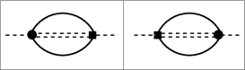
Figure 4: TR corrections to the self energies of spin-fermion propagators in the limit of weak magnetic field $h\ll|w_{d}|$. Circles and squares denote the vertices $\sim J$, which conserve and do not conserve the total spin, respectively (see the text for details.)

The explicit expressions for the self energy diagrams for $\hat{g}_{\perp}(\varepsilon)$ and $\hat{g}_{1}(\varepsilon)$ are,

$$\Sigma_{\perp}(\varepsilon)=\frac{S^{+}w_{d}+S^{-}w_{d}^{*}}{8h}\cdot\Sigma_{1}(\varepsilon)$$ (31)

$$\Sigma_{1}(\varepsilon)=J^{2}T^{2}\sum_{\omega_{1}\omega_{2},k_{1}k_{2}}G_{k_{1}}(-\omega_{1})G_{k_{2}}(\omega_{2})g_{1}(\varepsilon+\omega_{1}+\omega_{2})$$

Here $G_{k}(\omega)$ are the bare propagators for conduction electrons in the leads. In terms of real frequencies we find that the leading logarithmic term of this self energy has the form

$${\rm Re}\Sigma_{1}(\varepsilon)=2(\varrho_{0}J)^{2}h\ln\frac{D_{0}}{\max\{(|2\Delta-\varepsilon|),T\}},$$ (32)

(cf. similar estimates for self energies of spin fermion propagators describing singlet-triplet configuration in quantum dots with even occupation at finite bias KKM ). The imaginary part of the self energy ${\rm Im}\Sigma_{1}(\varepsilon)\sim J^{2}T$ is irrelevant. Inserting these estimates in (31), we find that this self energy enhances both real and imaginary parts of the planar magnetic field. At $T>|2\Delta-\varepsilon|$ corrections to the planar components of the effective magnetic fields may be estimated as

$$\frac{\delta w_{d}}{|w_{d}|}\sim(\rho_{0}J)^{2}\ln\frac{D_{0}}{T}.$$ (33)

Thus, we have found that the magnetic anisotropy induced by the TR precession is enhanced due to the interplay between this precession and the Kondo co-tunneling. In the limit of strong field $h\gg w_{d}$ this enhancement acquires the form of ”dynamical” contribution to the planar magnetic field. This ”random” field reminds the effect of exchange anisotropy induced by an edge spin coupled to an open spin-one-half antiferromagnetic Heisenberg chain.FraZ The Kondo-induced component of the planar field is weak at $T\gtrsim T_{K}$, $|\delta w|_{\perp}/T_{K}\sim j\Delta$. However, it generates its own energy scale

$$T^{*}=T_{K}\exp\left(-\frac{1}{j}\right)$$ (34)

where the precession induced magnetic field becomes comparable with the static magnetic field $\Delta$.

III.2 Weak magnetic field

In the limit of weak field (or strong TR interaction), namely, $w_{d}\gg h$, the general phenomenological analysis of Section II points toward another way to arrive at a Dzyaloshinskii-Moriya form for the TR corrections to the effective exchange Hamiltonian. Let us consider a model with nonlocal exchange between the dot and the leads with the effective exchange given by the Hamiltonian (15) in the absence of TR precession. Assume that the Rashba vectors are parallel in both lead and dot systems, $\vec{n}_{l}\parallel\vec{n}_{d}\parallel z$ but $w_{d}\neq w_{l}$. Then the spin Hamiltonian acquires the form (11).

In accordance with the kinematic scheme of Fig. 1, at zero magnetic field and square $(xy)$ symmetry, the Euler angles are $\Theta_{l}=\Theta_{d}=\pi/2$ and $\Phi_{l}=\Phi_{d}=\pi/4$. The difference between the coordinates $(x^{\prime\prime},y^{\prime\prime},z^{\prime\prime})$ for lead and dot spins at small $h$=$h_{z}$ is proportional to the deviation of $\Theta_{d}$ and $\Theta_{l}$ from $\pi/2$, namely $\pi/2-\Theta_{i}$=$\varphi_{i}$, where $\varphi_{i}\approx h/w_{i}$. Then the mismatch between the directions of the vectors $\vec{S}$ and $\vec{\sigma}_{R}$ is small like in Fig. 2, but the axis $\vec{n}$ is directed along the coordinate $z^{\prime\prime}=x$ of Fig. 1. Returning to the original frame $(x,y,x)$ we write the bare dot spin Hamiltonian in the form (19), and matching the angles $\Omega_{d}\to\Omega_{l}$ means applying the transformation

$$\vec{S}^{\prime}=\vec{S}+\varphi\ (\vec{n}\times\vec{S}),$$ (35)

where $\varphi=|\varphi_{d}-\varphi_{l}|$ and only the $x$-component of the vector product survives. The TR correction to the exchange Hamiltonian acquires the form

$$\delta H_{\rm cot}=\frac{i\varphi J}{2}\left[S_{z}(\sigma^{-}-\sigma^{+})+(S^{-}-S^{+})\sigma_{z}\right]$$ (36)

In this limit the main contribution to the spin-fermion propagators (24) is given by the off-diagonal components $g_{\sigma\bar{\sigma}}$, while the residues of the longitudinal components $g_{\sigma\sigma}$ contain small parameter $\varphi$. Thence the“anomalous” contribution to the Kondo loops (Fig. 4) gives the leading contribution to the scaling equations for the vertices $i\kappa=i\varphi J$ (36),

$$\frac{\partial\kappa}{\partial\eta}=-\kappa J~{}.$$ (37)

which implies scaling evolution of $\kappa$ similar to that of $j_{\mbox{\tiny TR}}$ (28), (29). Then we get an expression for the longitudinal component of the self energy given by the diagrams depicted in Fig. 4:

$$\Sigma_{\|}(\varepsilon)=\frac{i\varphi(w_{d}-w_{d}^{*})S_{z}}{4}\Sigma_{1}(\varepsilon).$$ (38)

As in Eq. (32), the logarithmic renormalization arises in the self energy for real frequencies, and the magnetic field enhancement can be estimated similarly to (33)

$$\frac{\delta h}{h}\approx(\rho_{0}J)^{2}\ln\frac{D_{0}}{\max\{|2\Delta-\varepsilon|,T\}}.$$ (39)

Thus we have found that the interplay between the Kondo scattering and the TR precession in case where the Rashba vector is parallel to a magnetic field results in logarithmic enhancement of the planar and the $z$-component of the effective magnetic field in the limits of strong and weak external field, respectively. This interplay disappears in zero field in agreement with the general symmetry considerations.Mewin

IV Conclusions

The main result of our analysis of the kinematics of Rashba effect in a system ’quantum dot plus metallic reservoir’ is the statement that the TR precession in one subsystem is ”exported” to another subsystem by the tunneling processes. This means that the TR precession always exists both in the dot and in the leads, and the inequality $\Theta_{d}\neq\Theta_{l}$ for the Euler angles related to the quantization axes in the two subsystems [see Eqs. (3) - (11)] arises in an external magnetic field, so that the magnetic quantization axes are never matched. In the limits of strong and weak magnetic field the Hamiltonian (11) is reducible to the Dzyaloshinsky – Moriya like form. This conclusion is quite general, and one may expect similar mismatch in complex quantum dots, where each constituent dot will be characterized by its own set of Euler angles $\Omega_{di}$.

As to the physical manifestations of the interplay between Kondo tunneling and Thomas – Rashba precession, the main effect is the sharp anisotropy of the g-factor due to the influence of the precession on the direction of the effective field $\vec{h}_{d}$ [see, e.g., Eq. (19)]. Due to the contributions of Kondo processes, this effect is temperature dependent and may be quite noticeable in case of weak magnetic field (39).

We restricted our study for the case of local TR effect in the leads (16). The theory may be generalized for the case of ”itinerant” quantization axis following the rotation of the quantization axis in the 2D Brillouin zone. In this case the higher angular harmonics of the electron states in the leadsMalec should be involved.

Acknowledgement The authors are grateful to M.N. Kiselev, A. Nersesyan and A.A. Zvyagin for valuable comments. Discussions with Y. Oreg at the initial stage of this work are highly appreciated.The research of Y.A is partially supported by an ISF grant 173/2008.

References

- (1) Yu.A. Bychkov and E.I. Rashba, J. Phys. C 17, 6039 (1984).
- (2) E.I. Rashba, in Problems of Condensed Matter Physics, eds. A.L. Ivanov and S.G. Tikhodeev (Oxford: Clarendon Press, 2006), p. 188.
- (3) Y. Meir and N.S. Wingreen, Phys. Rev. B 50, 4947 (1994).
- (4) K.V. Kavokin, Phys. Rev. B 69, 075302 (2004).
- (5) J. Malecki, J. Stat. Phys. 129, 741 (2007).
- (6) M. Zarea, S.E. Ulloa, and N. Sandler, Phys. Rev. Lett. 108, 046601 (2012).
- (7) L. Isaev, D.F. Agterberg, and I. Vekhter, Phys. Rev. B 85, 081107(R) (2012).
- (8) D. Sanchez, L. Serra, Phys. Rev. B 74, 153313 (2006)
- (9) R.Lopez, D. Sanchez, L. Serra, Phys. Rev. B 76, 035307 (2007).
- (10) Q. Q. Xu, B. L. Gao, and S. J. Xiong, Physica B 403, 1686 (2008).
- (11) L. Kouwenhoven and L. Glazman, Physics World, 14, 33 (2001).
- (12) T. Bergsten et al, Phys. Rev. Lett. 96, 076804 (2006).
- (13) M. König et al, Phys. Rev. Lett. 97, 196803 (2006).
- (14) T. Aono, Phys. Rev. B 76, 073304 (2007).
- (15) T. Moriya, in Magnetism, eds. T. Rado, H. Suhl (Academic Press, 1963), v.1 p. 86.
- (16) H. Imamura, P. Bruno, and Y. Utsumi, Phys. Rev. B 69, 121303 (2004).
- (17) J. Simonin, Phys. Rev.Lett. 97, 266804 (2006).
- (18) Q. F. Sun, Y. Wang, and H. Guo, Phys. Rev. B 71 (2005).
- (19) I. Affleck, A.W.W. Ludwig, H.-B. Pang, and D.L. Cox, Phys. Rev. B 45, 7918 (1992).
- (20) P.W. Anderson, J. Phys. C 3, 2436 (1970).
- (21) The analog of Eq. (26) is the local Green function for lead electrons in presence of TR splitting, which consists of two terms, . Both conduction subbands contribute to ”normal” and ”anomalous” Green function components.Imam
- (22) M.N. Kiselev, K. Kikoin and L.W. Molenkamp, Phys. Rev. B 68 155323 (2003).
- (23) H. Frahm and A.A. Zvyagin, J. Phys. CM 9, 9939 (1997).