The Carina Project. V. The impact of NLTE effects on the iron content

Abstract

We have performed accurate iron abundance measurements for 44 red giants (RGs) in the Carina dwarf spheroidal (dSph) galaxy. We used archival, high-resolution spectra ($R\sim 38\,000$) collected with UVES at ESO/VLT either in slit mode (5) or in fiber mode (39, FLAMES/GIRAFFE-UVES). The sample is more than a factor of four larger than any previous spectroscopic investigation of stars in dSphs based on high-resolution ($R\geq 38\,000$) spectra. We did not impose the ionization equilibrium between neutral and singly-ionized iron lines. The effective temperatures and the surface gravities were estimated by fitting stellar isochrones in the $V$, B–V color-magnitude diagram. To measure the iron abundance of individual lines we applied the LTE spectrum synthesis fitting method using MARCS model atmospheres of appropriate metallicity. For the 27 stars for which we measured both Fe I and Fe II abundances, we found evidence of NLTE effects between neutral and singly-ionized iron abundances. The difference is on average $\sim 0.1$ dex, but steadily increases when moving from the metal-rich to the metal-poor regime. Moreover, the two metallicity distributions differ at the 97% confidence level. Assuming that the Fe II abundances are minimally affected by NLTE effects, we corrected the Fe I stellar abundances using a linear fit between Fe I and Fe II stellar abundance determinations. We found that the Carina metallicity distribution based on the corrected Fe I abundances (44 RGs) has a weighted mean metallicity of $\hbox{[\rm{Fe/H}]}=-1.80$ and a weighted standard deviation of $\sigma=0.24$ dex. The Carina metallicity distribution based on the Fe II abundances (27 RGs) gives similar estimates ($\hbox{[\rm{Fe/H}]}=-1.72$, $\sigma=0.24$ dex). The current weighted mean metallicities are slightly more metal poor when compared with similar estimates available in the literature. Furthermore, if we restrict our analysis to stars with the most accurate iron abundances, $\sim$ 20 Fe I and at least three Fe II measurements (15 stars), we found that the range in iron abundances covered by Carina RGs ($\sim 1$ dex) agrees quite well with similar estimates based on high-resolution spectra. However, it is a factor of two/three smaller than abundance estimates based on the near-infrared Calcium triplet. This finding supports previous estimates based on photometric metallicity indicators.

1. Introduction

The Carina dSph galaxy is a fundamental benchmark to constrain the formation and evolution of dwarf galaxies and a key laboratory to improve current knowledge of low- and intermediate-mass stars’ evolutionary and pulsation properties (e.g. Smecker-Hane et al., 1999; Monelli et al., 2003; Bono et al., 2010). Quantitative constraints on its stellar content require not only precise multiband photometry over the entire body of the galaxy (Stetson et al., 2011), but also accurate measurements of the mean metallicity and of the spread, if any, in metallicity.

Using the multi-fiber spectrograph ARGUS at the CTIO 4 m Blanco telescope, Smecker-Hane et al. (1999) collected low-resolution ($R\sim 3\,000$) spectra for 52 Red Giants (RGs), covering the near-infrared (NIR) Calcium triplet (CaT) region, and found a mean metallicity of $\hbox{[\rm{Fe/H}]}=-1.99$ and a small spread in metallicity ($\sigma_{\rm[Fe/H]}=0.25$ dex). On the other hand, Koch et al. (2006) collected medium-resolution spectra ($R\sim 6\,500$) for 437 RGs with the multi-fiber spectrograph FLAMES/GIRAFFE (Pasquini et al., 2002) in MEDUSA mode at ESO/VLT,and using the same diagnostic found a mean metallicity of $\hbox{[\rm{Fe/H}]}=-1.90\pm 0.01$ (metallicity scale by Zinn & West 1984) and a significant spread in metallicity (full range $-3.0\lesssim\hbox{[\rm{Fe/H}]}\lesssim 0.0$). Koch et al. (2006) transformed the individual equivalent widths (EWs) of the CaT lines into iron abundances using the calibration provided by Rutledge et al. (1997). In a more recent investigation, Helmi et al. (2006) studied the same spectroscopic data and found a similar mean metallicity, ($\hbox{[\rm{Fe/H}]}=-1.7\pm 0.1$), but a smaller spread in iron abundance ($-2.3\lesssim\hbox{[\rm{Fe/H}]}\lesssim-1.3$). However, they used a different calibration between the EW of CaT lines and metallicity (Tolstoy et al., 2001) and different criteria for selecting candidate Carina stars. The difference between the two metallicity distributions appears as a steeper metal-rich tail in the latter distribution when compared with the former one.

High-resolution spectra ($R\sim 40\,000$) are available for a sample of five bright RG stars, collected with the slit mode of Ultraviolet and Visual Echelle Spectrograph (UVES) at ESO/VLT (Dekker et al., 2000). The mean metallicity found by Shetrone et al. (2003) from these spectra is $\hbox{[\rm{Fe/H}]}=-1.64$ with $\sigma_{\rm[Fe/H]}=0.4$ dex. The spread decreases to 0.25 dex if we remove the most metal-rich star in the sample. Independent measurements by Koch et al. (2008), using high-resolution ($R\sim 38\,000$) spectra for ten bright RGs collected with the red arm of UVES from FLAMES/GIRAFFE fibers, give a similar mean metallicity of $\hbox{[\rm{Fe/H}]}=-1.69$, but a spread that is a factor of two larger ($\sigma_{\rm[Fe/H]}=0.51$ dex).

A detailed spectroscopic analysis of Carina RGs was recently provided by Lemasle et al. (2012). They used FLAMES/GIRAFFE spectra for 35 RGs collected with grisms HR10 ($R\sim 19\,800$), HR13 ($R\sim 22\,500$) and HR14_new ($R\sim 17\,700$). They found a mean abundance based on Fe I lines ($\mu_{\rm[FeI/H]}=-1.63\pm 0.01$, $\sigma_{\rm[FeI/H]}=0.27$ dex, weighted mean) that agrees quite well with similar estimates available in the literature. On the other hand, the mean abundance based on Fe II lines ($\mu_{\rm[FeII/H]}=-1.24\pm 0.01$, $\sigma_{\rm[FeII/H]}=0.31$ dex, weighted mean) is slightly more metal-rich, but the difference is of the order of 1$\sigma$. Moreover and even more importantly, they found that their metallicity estimates range from $\hbox{[\rm{Fe\,{\scriptsize I}/H}]}=-1.2$ to $\hbox{[\rm{Fe\,{\scriptsize I}/H}]}=-2.5$, thus supporting a corresponding decrease in the metallicity spread.

A more recent analysis has been provided by Venn et al. (2012), using high-resolution spectra collected either with FLAMES/GIRAFFE-UVES (seven RGs) or with Magellan-MIKE ($R\sim 28\,000$, blue, $\sim 22\,000$, red, two RGs). They found, by using EWs, mean abundances based on Fe I ($\mu_{\rm[FeI/H]}=-1.79\pm 0.09$, $\sigma_{\rm[FeI/H]}=0.54$ dex, weighted mean) and on Fe II lines ($\mu_{\rm[FeII/H]}=-1.76\pm 0.09$, $\sigma_{\rm[FeII/H]}=0.53$ dex) that agree quite well with similar estimates available in literature.

Current spectroscopic investigations support the evidence that Carina may host very metal-poor stars ($\hbox{[\rm{Fe/H}]}<-3.0$, Helmi et al., 2006). This evidence, if supported by independent spectroscopic investigations, would imply that Carina underwent a fast chemical enrichment starting in a metal-poor environment and rapidly approaching a metal-intermediate regime ($\hbox{[\rm{Fe/H}]}\sim-1.6$).

Photometric investigations agree with the spectroscopic measurements concerning the mean metallicity, but suggest a small spread in metallicity ($\sigma_{\rm[Fe/H]}\sim 0.25$ dex, Bono et al. 2010; $\sigma_{\rm[Fe/H]}\sim 0.35$ dex, Lianou et al. 2011). In this work we perform a reanalysis of the Carina spectra investigated by Shetrone et al. (2003), Koch et al. (2008) and Venn et al. (2012) together with the analysis of a new high-resolution spectroscopic data set. In total we have 89 spectra for 72 stars. However, 18 of them are probable non-members, two of them are carbon stars, for six of them we have not been able to measure the radial velocity and for two of them we have not been able to measure the iron abundances. Overall, we provide new homogeneous iron abundance measurements for 44 Carina RGs based on high-resolution spectra collected with UVES (slit mode, five) and with FLAMES/GIRAFFE-UVES (multifiber mode, 39) at ESO/VLT.

This is the largest sample of high-resolution ($R\geq 38\,000$) spectra ever collected for a dSph galaxy. A similar spectroscopic approach was also adopted by Letarte et al. (2010) for RGs in the Fornax dSph. They used FLAMES/GIRAFFE spectra for 81 RGs collected with grisms HR10, HR13 and HR14_new. A set of spectra were also collected with the old version of the grism HR14_old ($R\sim 28\,800$), but they were rescaled to the resolution of the spectra collected with the grism HR14_new.

2. Observations and data reduction

The high-resolution spectra for Carina RGs adopted in this investigation were retrieved from the ESO Science Archive. We selected spectra from four different ESO/VLT observing programs collected with either UVES (slit mode, nine) or FLAMES/GIRAFFE-UVES (multifiber mode, 80).

The oldest (2000–2001) data set includes nine spectra of five RGs with visual magnitudes ranging from 17.62 to 17.92 mag. These spectra were collected with red arm of UVES, include 37 orders and have already been analyzed by Shetrone et al. (2003). The second (2003) data set comprises individual spectra for 33 RGs collected with the FLAMES/GIRAFFE-UVES red arm; their visual magnitudes range from 17.32 to 18.98 mag. The orders and the wavelength coverage of these spectra are the same as the UVES spectra. They have already been analyzed by Koch et al. (2008) who found that two of them are candidate carbon stars (stars Car54, Car55, or using Kock’s IDs, LG04a_000057 and LG04b_000569). We support the classification suggested by Koch et al. (2008), and have not included these stars in the current abundance analyses. The third (2005) data set and collected with FLAMES/GIRAFFE-UVES. The visual magnitudes of the RGs range from 17.65 to 18.00 mag. In the fourth (2007–2008) data set there are 40 spectra for 40 different stars collected with FLAMES/GIRAFFE-UVES, and their visual magnitudes range from 17.61 to 18.68 mag.

All the spectra collected with the red arm of UVES cover the wavelength range $4780-6825$ Å and the signal-to-noise ratio ($S/N$) is typically of the order of 30 ($\lambda\sim$ 6750 Å). The spectra collected with the FLAMES/GIRAFFE-UVES red arm cover the same wavelengths and have $S/N$ (at $\lambda\sim$ 6750 Å) ranging from $\sim$15$\pm$5 (21 stars) to $\sim$30$\pm$10 (11 stars) and $\sim$45$\pm$5 (7 stars).

We ended up with a sample of 89 high-resolution spectra for 72 stars, located across Carina’s central regions and covering the bright portion of the RG branch (see Fig. 1). We chose to use spectra taken with the red arm of UVES (centered at 5800 Å) because it is minimally affected by contamination from sky lines. The UVES spectra were reduced using IRAF, and extracted using the IRAF task apall. Wavelength calibration was performed using reference lines from (Murphy et al., 2007).

3. Radial velocity and photometric analysis

We measured the radial velocity ($RV$) of each spectrum following the same approach as adopted by Fabrizio et al. (2011), using two dozen heavy-element lines ranging from 6136 to 6200 Å. We measured the $RV$ of 66 stars (81 spectra). For six stars the measurement of the $RV$ was not possible due to the poor quality of the spectra. Among the stars with $RV$ measurements, 46 (61 spectra) are candidate Carina stars (with $212<RV<243$ km s^-1, Fabrizio et al. 2011). The others are either candidate field stars (18, $RV<100$ km s^-1) or candidate carbon stars (two) and they were not included in the current analysis.

To provide accurate estimates for the stellar parameters of the spectroscopic targets (effective temperature $T_{\mathrm{eff}}$ and surface gravity $\log g$), we used the multiband photometry discussed in Bono et al. (2010) and in Stetson et al. (2011). Moreover, we adopted different scaled-Solar cluster isochrones from the BaSTI data base (Pietrinferni et al., 2004, 2006). We selected isochrones at fixed age (12 Gyr) for three different chemical compositions ($\hbox{[\rm{Fe/H}]}=-1.50,-1.79,-2.27$). We also adopted a true distance modulus $DM_{0}=20.15$ mag and a reddening $E(B-V)=0.04$ mag (Dall’Ora et al., 2003). Finally, we performed a linear regression among the different isochrones and derived analytical relations connecting the visual magnitude $V$, the B–V color and either the surface gravity or the effective temperature. On the basis of the above relations and of the observed magnitudes and colors, we estimated the atmospheric parameters for each spectroscopic target. The adopted approach and the analytical relations will be described in a future paper (Ferraro et al. in preparation).

The top panel of Fig. 1 shows the position of the spectroscopic targets in the $V$, B–V Color-Magnitude Diagram (CMD) together with the entire photometric catalog (grey dots, Bono et al. 2010). The black dots mark the 46 candidate Carina stars, while the tiny orange dots display the 20 candidate field stars and the two large orange dots show the carbon stars. The blue squares and the red stars show the high-resolution sample of Koch et al. (2008) and Shetrone et al. (2003), respectively. The solid lines display the adopted isochrones. Taking into account current uncertainties in the Carina true distance modulus, the reddening, the mean metallicity (Dall’Ora et al., 2003; Pietrzyński et al., 2009; Bono et al., 2010; Lemasle et al., 2012) and the spread in age (Stetson et al., 2011), we performed a series of simulations and found that the typical uncertainties in temperature and gravity are $\epsilon_{T_{\mathrm{eff}}}\sim 70$ K and $\epsilon_{\log{g}}\sim 0.2$ dex (see Table 1). The bottom panel of Fig. 1 shows the same isochrones as the top panel, but in the $\log g$ vs $T_{\mathrm{eff}}$ plane together with the target stars. The error bars plotted in the bottom right corner represent the aforementioned uncertainties.

4. Spectroscopic analysis

The iron abundance analysis was performed following the classical spectrum-synthesis method for both Fe I and Fe II lines, but with one difference: we did not impose LTE ionization equilibrium between the Fe I and Fe II lines (e.g. Kraft & Ivans 2003). This means that we trust the surface gravity determined from the optical photometry and cluster isochrones. For the highest $S/N$ spectra collected with UVES, we selected Fe I and Fe II lines from the VALD data base (Kupka et al., 2000). We ended up with a list of 123 Fe I and 18 Fe II lines in the wavelength range covered by our spectra. Among them, 45 Fe I and 5 Fe II lines are located in overlapping orders.

By using the photometric estimates of both $T_{\mathrm{eff}}$ and $\log g$, and the Carina mean metallicity $\hbox{[\rm{Fe/H}]}=-1.70$ (Koch et al., 2008), we interpolated the MARCS model atmospheres (Gustafsson et al., 2008) with a modified version of the Masseron (2006) code for each Carina star. The individual models assumed spherical geometry, an $\alpha$-enhanced ($\hbox{\rm[$\alpha$/Fe]}=+0.4$) chemical mixture, a mass value of 1$M_{\odot}$ and a constant microturbulence velocity ($\xi=2$ km s^-1). The value adopted for the microturbulence velocity follows the estimates provided by Shetrone et al. (2003) for Carina red giants using metal-poor stellar model atmospheres. Similar estimates for the $\xi$ values were provided by Thévenin (1998) for RG stars with similar atmospheric parameters in the globular $\omega$ Cen. The Carina targets span a modest range in atmospheric parameters, therefore we decided to adopt the same $\xi$ value for the entire sample. The synthetic spectra were computed using the 1D, plane-parallel, LTE, radiative transfer code MOOG (2009 version, Sneden 1973). Note that plane-parallel radiative transfer for giant stars is more accurate when using spherical model atmospheres (Heiter & Eriksson, 2006).

We chose the Solar chemical composition from Grevesse et al. (2007), i.e., a Solar iron abundance of $A_{{\rm Fe}}^{\odot}=7.45$. Oscillator strengths $f$ for Fe I and Fe II lines are from VALD. When available, the parameters for collisional damping with neutral hydrogen are based on quantum theory (Anstee & O’Mara, 1995; Barklem & O’Mara, 1997; Barklem et al., 1998); otherwise the Unsöld classical recipe (Unsöld, 1955) was used with an enhanced damping factor of $F_{H}=1.5$. We note that calculations based on quantum theory are available for all the selected Fe II lines. The strategy adopted for the iron abundance analysis was dictated by the quality of the observations: high-resolution ($R\sim 38\,000$) and a reasonable signal-to-noise ratio ($15\lesssim S/N\lesssim 45$). We decided to use an eye fitting procedure rather than an automatic EW fitting procedure, since most of the weak lines are either noisy or blended.

The selected Fe I and Fe II lines were normalized using a linear fit of the local continuum identified by eye inspection. Using the MOOG code, we synthesized spectra with different metallicities. The synthetic spectra were convolved with a Gaussian broadening function to reproduce the instrumental resolution. We neglected the effect of stellar rotation. The fit of the lines (45 Fe I + 5 Fe II) that appear in two overlapping orders were treated independently and the iron abundance for these lines was estimated as a weighted mean. After a preliminary analysis of the stars with multiple spectra, we decided to neglect the spectra with lower $S/N$ and we only analyzed the best available spectrum for each star (46 spectra).

It is worth mentioning that in the abundance analysis we did not include lines with $\lambda<4920$ Å  to overcome subtle uncertainties with the coherent scattering by hydrogen in the continuum that was not included in MOOG (Sobeck et al., 2011). To constrain quantitatively the possible error in abundance in this wavelength range we computed the abundances of the three Fe I lines at 4924, 4950 and 4973 Å. We used a MARCS model atmosphere assuming $T_{\mathrm{eff}}=4500$ K, $\log g=1$  dex and $\hbox{[\rm{Fe/H}]}=-1.5$ with the code TURBOSPECTRUM(Alvarez & Plez, 1998) which accounts for the coherent scattering by hydrogen in the continuum. We found no significant difference with the abundance measurement based on the MOOG code, and indeed the differences in the cores of the lines represent less than five percent of the line equivalent widths.

We performed a first preliminary mean iron abundance analysis for each star. Subsequently, we computed a new set of model atmospheres using the same values of $T_{\mathrm{eff}}$ and $\log~{}g$, but using the new individual iron abundances. We also decided to use scaled-Solar ($\hbox{\rm[$\alpha$/Fe]}=0.0$) MARCS models, since detailed abundance measurements of RGs in nearby dwarf galaxies (Shetrone et al., 2003; Koch et al., 2008) indicates that they show only a mild enhancement in $\alpha$-elements. For stars with $\hbox{[\rm{Fe/H}]}<-2.0$, we used $\alpha$-enhanced models because the very metal-poor, scaled-Solar MARCS models are not available. In this new iron abundance analysis, we double checked all the iron measurements and rejected strong, noisy, blended or too weak Fe I and Fe II lines from the analysis. The adopted line list with wavelengths for both neutral and ionized iron lines is presented in Table 2 together with ion identification, excitation potential (EP) and $\log gf$ values. We ended up with 83 Fe I and 11 Fe II lines. Among them, 25 Fe I and 4 Fe II lines are located in overlapping orders. We performed several experiments with synthetic spectra and we found that the accuracy of the line fits ranges from 0.1 to 0.15 dex.

The atmospheric uncertainty in the line-by-line abundance measurements was estimated using the formula based on the EW uncertainty suggested by Cayrel (1988). In particular, we adopted a mean equivalent width $\rm\overline{EW}$ (typical values of the selected lines are $\sim 50$ mÅ for Fe I and $\sim 30$ mÅ for Fe II) and the $S/N$ of each individual spectral order (estimated using the IRAF task splot). The final iron abundance for each star was computed as the weighted mean of the line-by-line abundances. Individual weights were chosen as the inverse of the atmospheric uncertanties to limit the influence of the outliers.

For each star, in Table 2 are also listed the line-by-line EWs. The EWs were measured using the IRAF task splot, assuming a single Gaussian line profile, since the selected lines are not blended nor asymmetric. Typical uncertainty on the widths is of the order of 5%, and it is caused by the estimate of the continuum. It is worth mentioning that the EWs listed in Table 2 are only given for completeness of the current spectroscopic analysis. The iron abundances we provide are only based on the spectrum synthesis fitting method. The differences between our EWs and those measured by Shetrone et al. (2003) and Koch et al. (2008) are minimal (weighted mean, $\rm{EW_{our}-EW_{author}}\sim-5.4$ and $\sim 1.7$ mÅ, respectively). The difference with EWs provided by Lemasle et al. (2012) is larger (eleven stars in common, $\sim-22$ mÅ). The comparison between the EWs provided by Lemasle et al. (2012) and those by Koch et al. (2008) gives a similar difference (one star in common, $\sim-27$ mÅ). The difference with EWs provided by Venn et al. (2012) is quite smaller (seven stars in common, $\sim-13$ mÅ), and compared with EWs provided by Koch et al. (2008) gives a similar difference (three stars in common, $\sim-18$ mÅ).

5. Results and discussion

5.1. Detailed Fe I and Fe II stellar abundances

We measured [Fe I/H] for 44 stars and [Fe II/H] for 27 stars out of the 46 stars in our sample. On average, the former are based on more than twelve measurements (five stars have a single measurement), and the latter are based on more than three measurements (eight stars have a single measurement). The iron abundance was not measured in two metal-poor stars (Car17, Car26) because the lines available were noisy, blended or misidentified. The individual [Fe I/H] and [Fe II/H] abundance measurements and their atmospheric errors for the entire sample are listed in Table 2. The mean [Fe I/H] and [Fe II/H] abundances for the entire sample, with their weighted standard deviations are given in columns 10 and 12 of Table 1. Columns 11 and 13 list the number of Fe I and Fe II lines used to estimate the individual weighted mean abundances.

We carried out a more detailed analysis to constrain the impact that the adopted atmospheric parameters have on individual abundance measurements. To address this classical issue, we computed synthetic spectra with a series of model atmospheres at fixed chemical composition, changing the effective temperature by 100 K, the surface gravity by 0.3 dex and the microturbulence velocity by 0.5 km s^-1. Note that we are using generous estimates for the uncertainties affecting the atmospheric parameters (see §3). In particular, we selected the star Car23, since its effective temperature ($\sim 4400$ K) and surface gravity ($\sim 0.80$ dex) can be considered as average values for the entire sample. The results listed in Table 3 indicate that a change of 100 K in effective temperature causes a change in the mean Fe I and Fe II abundances of the order of 0.1 dex. On the other hand, a change of 0.3 dex in $\log g$ has a minimal impact on the Fe I abundance and a difference of the order of 0.15 dex for the Fe II abundance. The differences in abundance caused by a change of 0.5 km s^-1 in microturbulence velocity are of the order of 0.05 and 0.07 dex for the Fe I and Fe II abundances, respectively. These findings support the analysis performed by Koch et al. (2008) and indicate that plausible changes in the atmospheric parameters introduce changes in the inferred iron abundances smaller than 0.15 dex. To account for the uncertainties affecting the atmospheric parameters, the errors on the weighted mean metallicities listed in column 10 and 12 of Table 1 were estimated by summing in quadrature the weighted standard deviation with the three typical errors stated above.

The iron abundances of the 27 stars for which we have both [Fe I/H] and [Fe II/H] measurements (Table 1) indicate that the [Fe I/H] abundances are systematically lower than [Fe II/H]. The mean difference ranges from $\sim$0.1 to 0.2 dex (Car12, Car3). Five stars show an opposite trend, but their Fe II measurements are based on one or two lines, and two out of the five have Fe I measurements based on two lines.

The detailed iron abundance analysis for five Carina stars, covering the entire range of apparent magnitudes, is shown in Fig. 2. To validate the accuracy of our $T_{\mathrm{eff}}$ determinations, we plotted for each star the abundance of individual lines as a function of the Excitation Potential (EP) of the lines. We performed linear fits and found that the slopes are within $\pm 0.06$ dex/eV (see labeled values in Fig. 2), except for a few stars with a limited number of Fe I measurements. We tested the Fe I lines (left panels), since they are based on a larger number of measurements. The data plotted in Fig. 2 indicate that weighted standard deviations for Fe I and Fe II lines are on average $0.12$ and $0.18$ dex, respectively. We also checked the impact of a change in microturbulence velocity on star Car14 by assuming $\xi=2.5$ km s^-1. The slope changed by less than 0.02 dex/eV, since the saturated Fe I lines were not taken into account in the current analysis.

5.2. Comparison with previous investigations

To validate our abundance analysis, we performed a detailed comparison with similar measurements available in the literature. We defined the iron abundance difference $\Delta\hbox{[\rm{Fe/H}]}=\hbox{[\rm{Fe/H}]}_{\mathrm{our}}-\hbox{[\rm{Fe/H}]}_{\mathrm{author}}$ after shifting the $\hbox{[\rm{Fe/H}]}_{\mathrm{author}}$ to the Solar iron abundance that we used ($A_{\rm Fe}^{\odot}=7.45$, Grevesse et al. 2007). The data plotted in Fig. 3 show $\Delta\hbox{[\rm{Fe\,{\scriptsize I}/H}]}$ (left) and $\Delta\hbox{[\rm{Fe\,{\scriptsize II}/H}]}$ (right) versus our iron abundance. The vertical error bars are the sum in quadrature of our atmospheric dispersion and the errors given by the different authors, while the dotted lines display the 1 $\sigma$ difference.

We have five stars in common with Shetrone et al. (2003) (Car2, Car3, Car4, Car10, Car12). Their Solar iron abundance reference is 7.52 from Grevesse & Sauval (1998). The data plotted in the panels a) of Fig. 3 show that our iron abundances are systematically more metal-poor than those by Shetrone et al. (2003), especially for Fe I. The weighted mean and weighted standard deviation of the difference are $\mu_{\Delta\mathrm{[FeI/H]}}=-0.25\pm 0.07$, $\sigma_{\Delta\mathrm{[FeI/H]}}=0.17$ and $\mu_{\Delta\mathrm{[FeII/H]}}=-0.17\pm 0.11$, $\sigma_{\Delta\mathrm{[FeII/H]}}=0.14$ dex. Star Car3, the object with the largest discrepancy, suggests that the iron abundance from these authors is an overestimate. This hypothesis is supported by Koch et al. (2006) who found $\hbox{[\rm{Fe/H}]}=-1.93$ after accounting for the difference in the zero-point. This agrees better with our abundances ($\hbox{[\rm{Fe\,{\scriptsize I}/H}]}=-2.14$, $\hbox{[\rm{Fe\,{\scriptsize II}/H}]}=-1.97$) than with the Shetrone’s estimates ($\hbox{[\rm{Fe\,{\scriptsize I}/H}]}=-1.58$, $\hbox{[\rm{Fe\,{\scriptsize II}/H}]}=-1.56$, using our iron Solar abundance). Neglecting this star, our abundances agree quite well with the Shetrone et al. (2003) measurements, and indeed the differences decrease to $\mu_{\Delta\mathrm{[FeI/H]}}=-0.17\pm 0.08$, $\sigma_{\Delta\mathrm{[FeI/H]}}=0.07$ and $\mu_{\Delta\mathrm{[FeII/H]}}=-0.09\pm 0.12$, $\sigma_{\Delta\mathrm{[FeII/H]}}=0.04$ dex. We adopted the same MOOG radiative transfer code and the same MARCS model atmospheres (values of $T_{\mathrm{eff}}$ and $\log g$ similar), but we used more recent versions (2009 for MOOG and 2008 for MARCS). The microturbulence velocities adopted by Shetrone et al. (2003) range from 1.9 to 2.2 km s^-1 and are quite similar to the value we adopted. We also performed a series of tests to constrain the difference between the results of Shetrone et al. (2003) and the current abundances. The differences of EWs measured for this work (see Table 2) and those published by Shetrone et al. (2003, see their Table 4) is minimal (a few mÅ, see §4). The oscillator strengths they adopted come from the papers of the Lick-Texas group (Fulbright 2000, and references therein) and from the NISTon-line Atomic Spectra Database. We have already mentioned that our atomic data come from the VALD database, and it is very difficult to critically evaluate the accuracy of atomic data coming from different databases. This is the reason why we give a very low statistical weight to the stars in our sample with iron abundances based on only one or two lines. This evidence indicates that the discrepancies might result from the different approaches adopted to estimate the abundances. Their abundances were estimated using the EW fitting method and forcing ionization equilibrium between Fe I and Fe II, whereas we adopted spectrum synthesis fitting method and did not force ionization equilibrium. It is also worth noting that the number of Fe I and Fe II lines adopted by Shetrone et al. (2003) is three times larger than our selection.

We also have ten stars in common with Koch et al. (2008). In their spectroscopic analysis (see also Koch et al. 2006), these authors adopted the metallicity scale of Carretta & Gratton (1997). Therefore, we assumed that they adopted a Solar iron abundance of 7.52. The comparison, after the shift in the zero-point, is shown in panels b) of Fig. 3. We found that we agree, within 1$\sigma$, with these authors for the Fe II abundance with $\mu_{\Delta\mathrm{[FeII/H]}}=-0.21\pm 0.08$ and $\sigma_{\Delta\mathrm{[FeII/H]}}=0.27$ dex. For Fe I the discrepancy is larger, with $\mu_{\Delta\mathrm{[FeI/H]}}=-0.34\pm 0.07$ and $\sigma_{\Delta\mathrm{[FeI/H]}}=0.26$ dex. In this case the difference in the abundances might be due to a difference either in the approach (EW versus spectrum-synthesis fitting methods) or in the input physics (or both). As a matter of fact, Koch et al. (2008) adopted their oscillator strengths from the standard RG star Arcturus. Moreover, they used Castelli & Kurucz (2003) model atmospheres, while we used MARCS models and their surface gravities are on average 0.3–0.5 dex higher than ours. The difference in gravity is the consequence of the different approach in estimating the gravity (forcing the balance between Fe I and Fe II versus photometric gravities).

We compared the current Fe I and Fe II abundances with similar abundances recently provided by Lemasle et al. (2012) from FLAMES/GIRAFFE spectra with a spectral resolution that is on average a factor of two smaller than ours. The data plotted in the panels c) of Fig. 3 show that the differences, after correcting for their reference Solar iron abundance (Grevesse & Sauval, 1998), in the Fe I abundances ($\mu_{\Delta\mathrm{[FeI/H]}}=-0.27\pm 0.09$ dex, weighted mean) and in the dispersion ($\sigma_{\Delta\mathrm{[FeI/H]}}=0.16$) for the eleven stars in common are quite similar to the results based on the other high-resolution estimates. The difference in the Fe II abundances is based on only four objects and attains similar values, namely $\mu_{\Delta\mathrm{[FeII/H]}}=-0.61\pm 0.27$, $\sigma_{\Delta\mathrm{[FeII/H]}}=0.25$ dex. Note that our [Fe II/H] abundance for the star with the largest discrepancy is based on only three Fe II lines.

Finally, we compared our Fe I and Fe II abundances with similar abundances provided by Venn et al. (2012) using EWs of FLAMES/GIRAFFE-UVES spectra. The data plotted in the panels d) of Fig. 3 show that the Fe I abundances for the seven stars in common, after correcting for their reference Solar iron abundance (Asplund et al., 2009), ($\mu_{\Delta\mathrm{[FeI/H]}}=-0.37\pm 0.11$ dex, weighted mean) and their dispersion ($\sigma_{\Delta\mathrm{[FeI/H]}}=0.19$) agree quite well with current estimates. The difference in the Fe II abundances is based on six objects and attains similar values, namely $\mu_{\Delta\mathrm{[FeII/H]}}=-0.26\pm 0.13$, $\sigma_{\Delta\mathrm{[FeII/H]}}=0.11$ dex.

We also compared our iron abundances to similar estimates by Koch et al. (2006). These authors performed detailed measurements of CaT EW for 437 RGs and transformed the reduced EWs into iron abundances, using the metallicity scales from Zinn & West (1984, ZW84) and Carretta & Gratton (1997, CG97). We compared their Fe I abundance estimates with our measurements of Fe I abundances. We have 25 stars with at least two iron line measurements in common with this sample and we found that the differences in the ZW84 and the CG97 metallicity scales are: $\mu_{{\Delta\mathrm{[Fe/H]}}}=-0.14\pm 0.04$ ($\sigma_{{\Delta\mathrm{[Fe/H]}}}=0.15$) and $\mu_{{\Delta\mathrm{[Fe/H]}}}=-0.33\pm 0.04$ ($\sigma_{{\Delta\mathrm{[Fe/H]}}}=0.18$) dex (see Fig. 4). Our iron abundances are slightly more metal-poor, but within 1 $\sigma$ and in better agreement with the ZW84 than with the CG97 metallicity scale. The difference of 0.2 dex between the ZW84 and the CG97 scale is well known (Carretta & Gratton, 1997; Kraft & Ivans, 2003).

5.3. Carina metallicity distribution

The data plotted in the top panels of Fig. 5 show the weighted metallicity distributions of our sample based on Fe I (left) and on Fe II (right) measurements. To constrain the metallicity distribution, we assigned to each star a Gaussian kernel (Di Cecco et al., 2010) with a $\sigma$ equal to the standard deviation of the iron abundance measurement. The solid lines were computed by summing the individual Gaussian over the entire data set (see panels a and b in Fig. 5). We found that both the median ($-1.84$ dex) and the weighted mean ($\mu_{\mathrm{[FeI/H]}}=-1.90\pm 0.02$ dex) of Fe I abundances (44 stars) attain similar values. The same outcome applies to the Fe II measurements (27 stars) for which we determined $\mu_{\mathrm{[FeII/H]}}=-1.72\pm 0.04$ dex. The weighted standard deviations attain small values ($\sim 0.25$ dex), but the metallicity distributions cover at least one dex. We also estimated the metallicity distribution by giving equal weight to all stars, and the difference with the weighted mean is minimal ($<0.04$ dex).

To constrain the dependence of these results on the accuracy of the abundance analysis, we recomputed the metallicity distribution using only stars with more than twelve Fe I and two Fe II line measurements (see panels c and d in Fig. 5). The weighted means and the weighted standard deviations reach values similar to those from the entire sample, but the range in metallicity decreases by at least 0.2 dex. The difference is mainly in the metal-poor tail, and indicates that high-quality spectra are required to constrain the actual dispersion in iron abundance of Carina RGs. To further constrain the impact of the abundance precision on the metallicity distribution we selected the stars with at least three Fe II line measurements. The Fe I metallicity distribution of the same stars is typically based on $\sim 20$ Fe I lines. We ended up with a sample of 15 stars, and the weighted mean for the Fe I metallicity distribution is slightly more metal-rich $\mu_{{\mathrm{[FeI/H]}}}=-1.77\pm 0.04$ dex, while the $\sigma_{{\mathrm{[FeI/H]}}}$ decreases to 0.19 dex. The same outcome applies to the Fe II metallicity distributions. Interestingly enough, the Fe I and Fe II metallicity distributions (see panels e and f in Fig. 5) cover a range of $\sim 1$ dex. The use of the best data indicates that the spread in metallicity of Carina RGs is smaller than previous estimates. Note that this finding appears to be minimally affected by selection biases, since the metal-poor stars ($\hbox{[\rm{Fe\,{\scriptsize I}/H}]}\leq-2.20$) not included in the metallicity distribution of panel e) cover the same range in luminosity as the selected stars. However, these findings call for new abundance analyses to constrain the real extent of the metal-poor tail of Carina.

By taking into account the 27 stars for which we determined both Fe I and Fe II abundances, we found that the weighted mean based on Fe I lines is 0.12 dex lower than the weighted mean based on Fe II lines. The difference brings forward the possible occurrence of NLTE effects between Fe I and Fe II abundances. Our experiment appears appropriate to constrain this effect, since we relaxed the constraint on the ionization equilibrium between Fe I and Fe II lines. This is an interesting finding, since detailed calculations and the comparison between theory and observations (Thévenin & Idiart, 1999; Thévenin et al., 2001; Mashonkina et al., 2011) show that the NLTE effects strongly affect the less abundant species (i.e., Fe I) which is over-ionized in RGs, in particular in metal-poor stars. This effect explain why the LTE ionization equilibrium between neutral and singly-ionized iron is destroyed and why we do not force [Fe I/H] to be equal to [Fe II/H] by decreasing the surface gravity. Note that for the five stars in common with Shetrone et al. (2003) we have on average larger $\log g$ values by 0.2 dex, but they decreased their photometric estimates of $\log g$ by $-0.29$ dex. The decrease in the $\log g$ values artificially forces the ionization equilibrium and causes an increase in their Fe I abundance determination. This approach partially overcome the NLTE effects by changing the surface gravity. The more abundant species (i.e., Fe II) are supposed to be free from NLTE effects, at least on the ionization equilibrium.

5.4. The impact of NLTE effects

To further constrain this effect, we directly compared Fe I and Fe II abundances. Data plotted in panels a), b) and c) of Fig. 6 indicate that the difference appear to increase when moving from metal-rich to metal-poor stars. We performed a linear fit (panel a, red dashed line, the zero-point $\alpha$ and the slope $\beta$ are labeled) over the 27 stars for which we have both Fe I and Fe II measurements. We found that the two metallicity distributions differ at the $\sim$97% confidence level. To further constrain this effect, we performed the same analysis, but using stars with abundances based on at least two Fe II lines (panel b). The sample decreased to 19 stars, but the two distributions still differ at the $\sim$87% confidence level. The outcome is the same if we use stars with abundances based on at least three Fe II lines (panel c), 15 stars, $\sim$75% confidence level.

On the basis of this empirical evidence, we corrected the Fe I abundances to account for the NLTE effects by using the linear fit between Fe I and Fe II abundances plotted as a red dashed line in panel a) of Fig. 6. The new Fe I metallicity distributions accounting for the NLTE effects are plotted as red dashed lines in panels a), c) and e) of Fig. 5. The weighted mean Fe I metallicity increases by $\sim$0.1 dex, while the weighted standard deviations attain similar values. The use of linear fits based on more accurate Fe II abundances for either 19 (panel b) or 15 (panel c) stars gives similar changes in the metallicity distributions. These results indicate that the weighted mean metallicity of the Carina RGs, corrected for NLTE effects, ranges from $\mu(\mathrm{NLTE})=-1.68$ (15 stars) to $-1.80$ (44 stars), while the weighted standard deviation ranges from 0.18 to 0.24 dex. The extreme range in iron abundance covered by the stars with the most accurate measurements is $\sim$1 dex.

In order to constrain the NLTE effects we performed NLTE computations for two metal abundances ($\hbox{[\rm{Fe/H}]}=-2.0,-1.5$) using the Fe I/II atom model provided by Collet et al. (2005). Note that to constrain the slope of the NLTE effects between Fe I and Fe II lines, the two MARCS model atmospheres used in NLTE computations have the same effective temperature (4500 K) and the same surface gravity (1.0 dex). The calculations were performed following the approach adopted by Thévenin & Idiart (1999) and by Collet et al. (2005). Moreover, we did not use inelastic collisions for supergiants as suggested by Merle et al. (2011), so our errors on NLTE abundances have to be considered as upper limits. We found significant NLTE effects in both Fe I and Fe II lines. Moreover, we found a significant relative difference between [Fe I/H] and [Fe II/H] theoretical abundances. A glance at the data plotted in Fig. 7 displays that the predicted slope agrees quite well with the observed one. In particular, the NLTE computations show stronger effects on Fe I than on Fe II abundances ($\sim 0.1$ dex). However, more detailed calculations accounting for changes in effective temperature and gravity are required before we can reach firm conclusions concerning the impact of NLTE effects on Fe I and Fe II abundances. The current findings do not demonstrate but further support the results obtained by Bergemann et al. (2011) concerning the occurrence of NLTE effects in metal-poor RG atmospheres. Finally, we note that our preliminary calculations also show non-negligeable NLTE effects on the Fe II lines. This finding, once confirmed by more detailed and independent calculations, implies that the true mean [Fe II/H] abundance of Carina stars should be increased by at least 0.1 dex.

6. Final remarks

The current findings soundly support previous estimates of Carina’s mean metallicity based on the difference in color between the Red Clump (RC) stars and the horizontal-branch (HB) at mean color of RR Lyrae $\hbox{[\rm{Fe/H}]}(\Delta(B-I)^{RC}_{HB})=-1.70\pm 0.19$ (Bono et al., 2010). The same outcome applies to the mean metallicity estimated using stellar isochrones $\hbox{[\rm{Fe/H}]}\sim-1.79$ (BaSTI data base, Stetson et al. 2011), $\hbox{[\rm{Fe/H}]}\sim-1.79\pm 0.35$ (Lianou et al., 2011). High-resolution spectra for 15 stars support, together with similar results available in the literature (Lemasle et al., 2012), a significant decrease in the range in iron abundances when compared with similar measurements based on CaT ($\sim 1$ vs 2–3 dex). The same conclusion applies to the comparison with the metallicity distribution predicted by chemical evolution models based on star formation histories available in the literature (Lanfranchi et al., 2006).

Our sample is more than a factor of four larger than any previous spectroscopic investigation based on high-resolution spectra. However, the current data do not allow us to determine whether the spread is either atmospheric, i.e., caused by a difference in the mean metallicity between the old and the intermediate-age population, or by measurement errors. To assess whether the different stellar populations are also characterized by different mean metallicities, new spectra with high $S/N$ down to RC (intermediate-mass) and to red HB (low-mass) stars are required.

We determined the mean iron abundance for a sample of 44 Carina RG stars. We corrected for NLTE effects on the ionization equilibrium and we found $\hbox{[\rm{Fe/H}]}=-1.80$ and $\sigma=0.24$ dex. If this estimate of Carina’s mean metallicity is supported by future, the position of this dSph in the Metallicity-Luminosity diagram will be between one and two $\sigma$ more metal-rich than expected according to the empirical relation followed by dSph, dE/dS0 and giant early type galaxies (Mateo, 2008; Chilingarian et al., 2011). If this turns out to be the case, it might open new issues concerning the interplay between chemical evolution and enrichment, star formation history and stellar evolution in gas-poor stellar systems (Walker et al., 2009; Revaz & Jablonka, 2012).

Table 1Atomic Data and Individual Iron Abundances

				Car2		Car3		Car4		Car10
$\lambda$ (Å)	Elem.	EP (eV)	$\log gf$	[Fe/H]	EW	[Fe/H]	EW	[Fe/H]	EW	[Fe/H]	EW
4924.770	26.0	2.279	$-2.241$	…	…	…	…	…	…	…	…
4950.110	26.0	3.417	$-1.670$	…	…	…	…	…	…	…	…
4973.100	26.0	3.960	$-0.950$	…	…	$-2.20\pm 0.14$	88	…	…	…	…
5044.210	26.0	2.851	$-2.038$	…	…	$-2.15\pm 0.13$	93	…	…	$-2.10\pm 0.12$	51
5054.640	26.0	3.640	$-1.921$	…	…	…	…	…	…	…	…
5090.770	26.0	4.256	$-0.400$	…	…	…	…	…	…	…	…
5197.580	26.1	3.230	$-2.348$	$-1.55\pm 0.30$	105	$-1.85\pm 0.38$	117	$-1.49\pm 0.42$	105	$-2.00\pm 0.21$	73
5215.180	26.0	3.266	$-0.871$	…	…	…	…	…	…	…	…
5217.390	26.0	3.211	$-1.070$	…	…	…	…	…	…	…	…
5234.620	26.1	3.221	$-2.279$	…	…	$-1.95\pm 0.34$	83	…	…	…	…
5242.490	26.0	3.634	$-0.967$	…	…	$-2.05\pm 0.17$	98	…	…	…	…
5264.810	26.1	3.230	$-3.133$	…	…	…	…	…	…	…	…
5284.110	26.1	2.891	$-3.195$	…	…	…	…	$-1.55\pm 0.20$	65	…	…
5288.520	26.0	3.694	$-1.508$	$-1.65\pm 0.13$	52	…	…	$-1.70\pm 0.24$	56	…	…
5307.360	26.0	1.608	$-2.987$	…	…	…	…	…	…	…	…
5316.620	26.1	3.153	$-2.014$	…	…	$-2.05\pm 0.20$	156	…	…	…	…

Table 2Impact of uncertainties in effective temperature, surface gravity and microturbulence velocity on iron abundances for the representative star Car23.

	$\Delta T_{\mathrm{eff}}$ [K]		$\Delta\log g$ [$\log(\rm{cm\>s^{-2}})$]		$\Delta\xi$ [km s-1]
Ion	$-100$	$+100$	$-0.3$	$+0.3$	$-0.5$	$+0.5$	$<$$\sigma$$>$
Fe I	$+0.10$	$-0.11$	$-0.01$	$-0.00$	$-0.10$	$-0.01$	$0.11$
Fe II	$+0.02$	$+0.10$	$-0.02$	$+0.13$	$-0.09$	$-0.04$	$0.12$

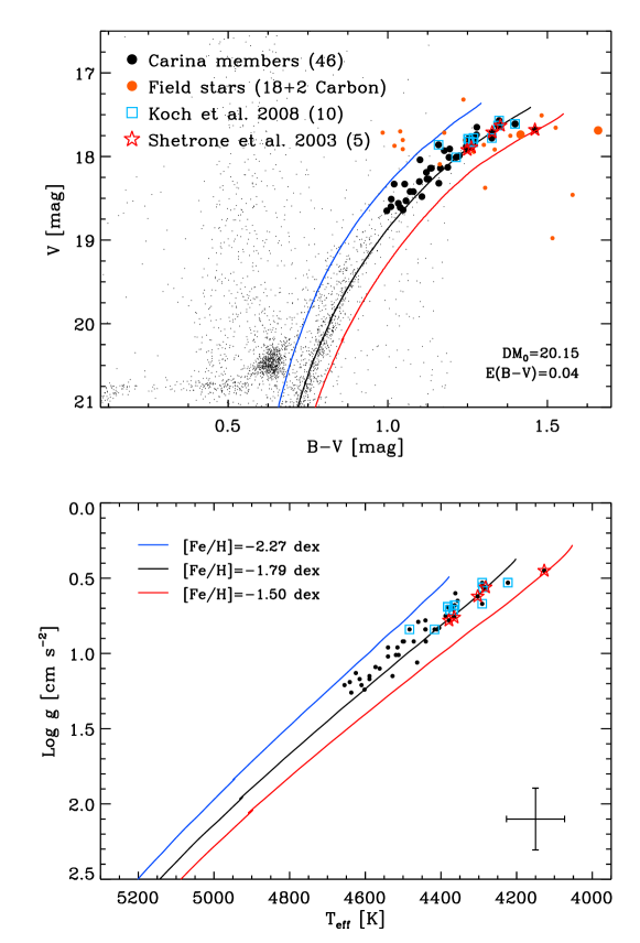
Figure 1.— Top: $V$, B–V CMD of the spectroscopic targets. The black dots mark the UVES targets with a $RV$ between 180 and 260 km s^-1 (Carina candidate members), while the small orange dots show targets with $RV$ outside the previous range (field stars). The two large orange dots refer to the two carbon stars. The blue squares and red stars mark the targets in common with the sample of Koch et al. (2008) and Shetrone et al. (2003). The colored lines show three scaled Solar isochrones (Pietrinferni et al., 2004, 2006) at the same age ($t=12$ Gyr) with $\hbox{[\rm{Fe/H}]}=-1.50$ in red, $\hbox{[\rm{Fe/H}]}=-1.79$ in black and $\hbox{[\rm{Fe/H}]}=-2.27$ in blue. The background gray dots are from the Carina photometric catalog (Bono et al., 2010). Bottom: Same as the top, but the targets are plotted in the effective temperature vs surface gravity plane. The error bars display typical uncertainty on both effective temperature and surface gravity.

Figure 2.— Detailed iron abundances as a function of the Excitation Potential (EP) for five stars covering the range in visual magnitude of the entire sample. From top to bottom the panels show for each star the line-by-line analysis for the Fe I abundance (left panels) and for the Fe II abundance (right panels). For each ionization stage, the mean weighted value and the statistical error are given and plotted as a dotted line. Numbers in square brackets are the number of iron lines used to measure the abundance.

Figure 3.— Panels a): Difference $\Delta\hbox{[\rm{Fe/H}]}=\hbox{[\rm{Fe/H}]}_{{\rm our}}-\hbox{[\rm{Fe/H}]}_{\rm author}$ in Fe I (left) and in Fe II (right) stellar abundances between our measurements and similar measurements by Shetrone et al. (2003). The weighted mean $\mu$ (thick lines) and the weighted standard deviation $\sigma$ are labeled together with the 1 $\sigma$ interval (dotted lines). The error bars display individual uncertainties of the two sets of abundances. Panels b): Same as panels a), but the difference is with similar measurements from Koch et al. (2008). Panels c): Same as panels a), but the difference is with similar measurements from Lemasle et al. (2012). Panels d): Same as panels a), but the difference is with similar measurements from Venn et al. (2012).

Figure 4.— Difference in iron abundance (as in Fig. 3) for the 25 Carina stars in common with Koch et al. (2006). They estimated stellar iron abundances from the CaT measurements based on medium-resolution spectra in the ZW84 (left) and in the CG97 (right) metallicity scale.

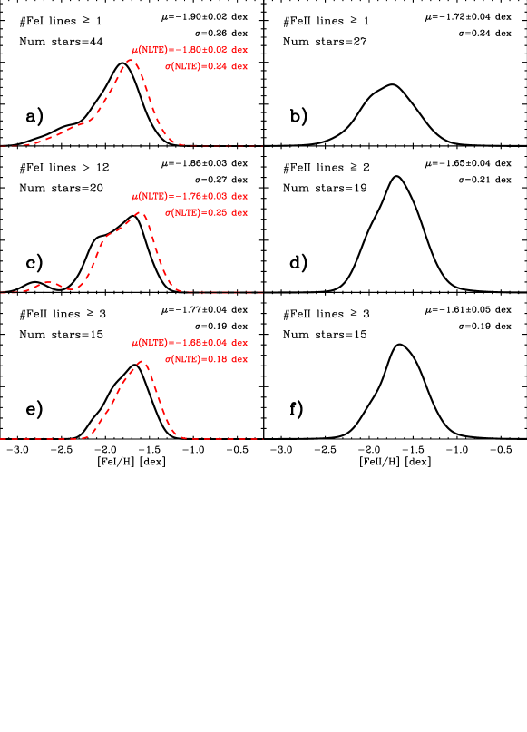
Figure 5.— Panels a)–b): Metallicity distributions of Carina stars based on Fe I (left) and Fe II (right) lines. The weighted means and the weighted standard deviations are labeled, together with the sample size. The red dashed line shows the Fe I metallicity distribution of the same stars, but accounting for NLTE effects. The correction of individual abundances is based on the linear fit between Fe I and Fe II abundances given in panel a) of Fig. 6. The new $\mu$(NLTE) and $\sigma$(NLTE) values are labeled in red. Panels c)–d): Same as the top, but for stars with more than twelve Fe I or with at least two Fe II measurements. Panels e)–f): Same as the top, but for stars with at least three Fe II measurements.

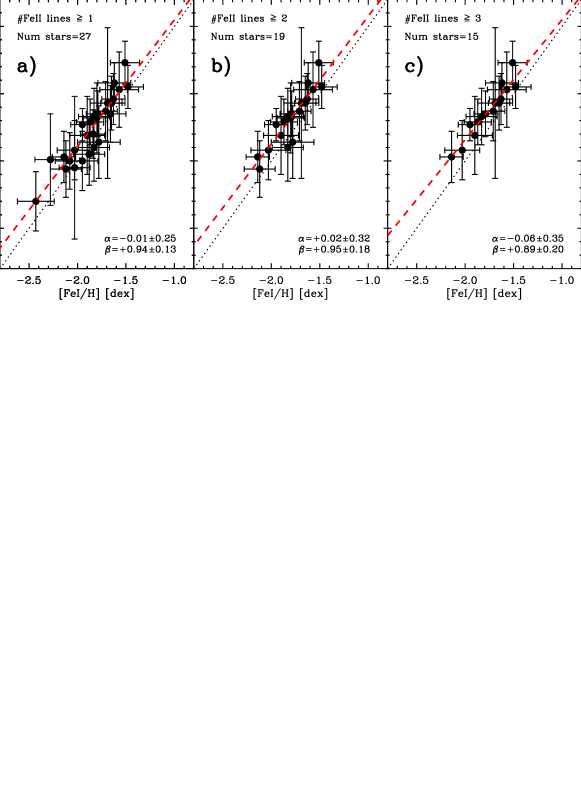
Figure 6.— Panel a): Comparison between stellar iron abundances based on neutral and on singly-ionized lines. The red dashed line shows the linear fit of the data, used to correct the Fe I metallicity distribution for NLTE effects. The zero-point ($\alpha$) and the slope ($\beta$) of the linear fit are labeled. Panels b) and c): Same as panel a), but for stars with at least two and at least three Fe II measurements, respectively.

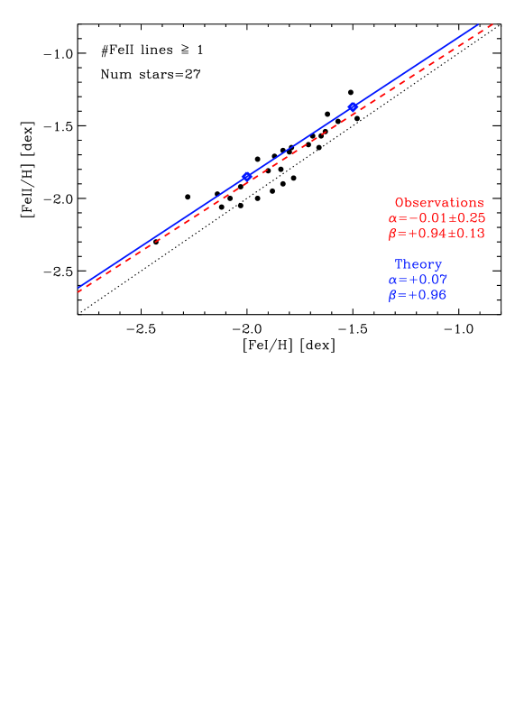
Figure 7.— NLTE effects on ionization equilibrium. The symbols (black dots) are the same as in panel a) of Fig. 6. The blue diamonds are the abundances given by NLTE computations of Fe I/II for two representative models of Carina RGs. We adopted an effective temperature of 4500 K, a surface gravity of 1.0 dex and two iron abundances $\hbox{[\rm{Fe/H}]}=-2.0,-1.5$. The dashed red line shows the linear regression on the data (the same as in panel a of Fig. 6), while the solid blue line shows the linear fit on the two NLTE models. The zero-point ($\alpha$) and the slope ($\beta$) of the linear fits are labeled.

References

- Alvarez & Plez (1998) Alvarez, R., & Plez, B. 1998, A&A, 330, 1109
- Anstee & O’Mara (1995) Anstee S. D., O’Mara B. J., 1995, MNRAS, 276, 859
- Asplund et al. (2009) Asplund, M., Grevesse, N., Sauval, A. J., & Scott, P. 2009, ARA&A, 47, 481
- Barklem & O’Mara (1997) Barklem P. S., O’Mara B. J., 1997, MNRAS, 290, 102
- Barklem et al. (1998) Barklem P. S., O’Mara B. J., Ross J. E., 1998, MNRAS, 296, 1057
- Bergemann et al. (2011) Bergemann, M., Lind, K., Collet, R., & Asplund, M. 2011, Journal of Physics Conference Series, 328, 012002
- Bono et al. (2010) Bono, G., et al. 2010, PASP, 122, 651
- Carretta & Gratton (1997) Carretta, E., & Gratton, R. G. 1997, A&AS, 121, 95
- Castelli & Kurucz (2003) Castelli, F., & Kurucz, R. L. 2003, Modelling of Stellar Atmospheres, 210, 20P
- Cayrel (1988) Cayrel, R. 1988, in IAU Symp. 132, The Impact of Very High S/N Spectroscopy on Stellar Physics, ed. G. Cayrel de Strobel & M. Spite (Dordrecht: Kluwer), 345
- Collet et al. (2005) Collet, R., Asplund, M., & Thévenin, F. 2005, A&A, 442, 643
- Chilingarian et al. (2011) Chilingarian, I. V., Mieske, S., Hilker, M., & Infante, L. 2011, MNRAS, 412, 1627
- Dall’Ora et al. (2003) Dall’Ora, M., et al. 2003, AJ, 126, 197
- Dekker et al. (2000) Dekker, H., D’Odorico, S., Kaufer, A., Delabre, B., & Kotzlowski, H. 2000, Proc. SPIE, 4008, 534
- Di Cecco et al. (2010) Di Cecco, A., et al. 2010, ApJ, 712, 527
- Fabrizio et al. (2011) Fabrizio, M., et al. 2011, PASP, 123, 902,
- Fulbright (2000) Fulbright, J. P. 2000, AJ, 120, 1841
- Grevesse et al. (2007) Grevesse N., Asplund M., Sauval A. J., 2007, Space Sci Rev, 130, 105
- Grevesse & Sauval (1998) Grevesse N., Sauval A. J., 1998, Space Sci Rev, 85, 161
- Gustafsson et al. (2008) Gustafsson B., Edvardsson B., Eriksson K., Jorgensen U. G., Nordlund Å, Plez B., 2008, A&A, 486, 951
- Heiter & Eriksson (2006) Heiter U., Eriksson K., 2006, A&A, 452, 1039
- Helmi et al. (2006) Helmi, A., et al. 2006, ApJ, 651, L121
- Koch et al. (2006) Koch, A., Grebel, E. K., Wyse, R. F. G., Kleyna, J. T., Wilkinson, M. I., Harbeck, D. R., Gilmore, G. F., & Evans, N. W. 2006, AJ, 131, 895
- Koch et al. (2008) Koch, A., Grebel, E. K., Gilmore, G. F., Wyse, R. F. G., Kleyna, J. T., Harbeck, D. R., Wilkinson, M. I., & Wyn Evans, N. 2008, AJ, 135, 1580
- Kraft & Ivans (2003) Kraft, R. P., & Ivans, I. I. 2003, PASP, 115, 143
- Kupka et al. (2000) Kupka F., Ryabchikova T. A., Piskunov N. E., Stempels H.C., Weiss W.W., 2000, Baltic Astronomy, vol. 9, 590-594
- Lanfranchi et al. (2006) Lanfranchi, G. A., Matteucci, F., & Cescutti, G. 2006, A&A, 453, 67
- Lemasle et al. (2012) Lemasle, B., Hill, V., Tolstoy, E., et al. 2012, A&A, 538, A100
- Letarte et al. (2010) Letarte, B., Hill, V., Tolstoy, E., et al. 2010, A&A, 523, A17
- Lianou et al. (2011) Lianou, S., Grebel, E. K., & Koch, A. 2011, A&A, 531, A152
- Masseron (2006) Masseron, T. 2006, PhD Thesis, Obs. de Paris
- Mateo (1998) Mateo, M. L. 1998, ARA&A, 36, 435
- Mateo (2008) Mateo, M. 2008, The Messenger, 134, 3
- Mashonkina et al. (2011) Mashonkina, L., Gehren, T., Shi, J.-R., Korn, A. J., Grupp, F., 2011 A&A, 528, A87
- Merle et al. (2011) Merle, T., Thévenin, F., Pichon, B., & Bigot, L. 2011, MNRAS, 418, 863
- Monelli et al. (2003) Monelli, M., et al. 2003, AJ, 126, 218
- Mould et al. (1982) Mould, J. R., Cannon, R. D., Frogel, J. A., & Aaronson, M. 1982, ApJ, 254, 500
- Murphy et al. (2007) Murphy, M.T., Tzanavaris,P., Webb,J.K., Lovis, C., 2007, MNRAS, 376,673.
- Pasquini et al. (2002) Pasquini, L. et al. 2002, The Messenger 110, 1
- Pietrinferni et al. (2004) Pietrinferni, A., Cassisi, S., Salaris, M., Castelli, F. 2004, ApJ, 612, 168
- Pietrinferni et al. (2006) Pietrinferni, A., Cassisi, S., Salaris, M., Castelli, F. 2006, ApJ, 642, 797
- Pietrzyński et al. (2009) Pietrzyński, G., Górski, M., Gieren, W., Ivanov, V. D., Bresolin, F., & Kudritzki, R.-P. 2009, AJ, 138, 459
- Revaz & Jablonka (2012) Revaz, Y., & Jablonka, P. 2012, A&A, 538, A82
- Rutledge et al. (1997) Rutledge, G. A., Hesser, J. E., Stetson, P. B., et al. 1997, PASP, 109, 883
- Shetrone et al. (2003) Shetrone, M., Venn, K. A., Tolstoy, E., Primas, F., Hill, V., & Kaufer, A. 2003, AJ, 125, 684
- Smecker-Hane et al. (1999) Smecker-Hane, T. A., Mandushev, G. I., Hesser, J. E., Stetson, P. B., Da Costa, G. S., & Hatzidimitriou, D. 1999, Spectrophotometric Dating of Stars and Galaxies, 192, 159
- Sneden (1973) Sneden C., 1973, ApJ, 184, 839
- Sobeck et al. (2011) Sobeck, J. S., Kraft, R. P., Sneden, C., et al. 2011, AJ, 141, 175
- Stetson et al. (2011) Stetson, P. B., et al. 2011, The Messenger, 144, 32
- Thévenin (1998) Thévenin, F. 1998, VizieR Online Data Catalog, 3193, 0
- Thévenin & Idiart (1999) Thévenin, F., Idiart, T. 1999, ApJ, 521, 753
- Thévenin et al. (2001) Thévenin, F., Charbonnel, C., de Freitas Pacheco, J. A., Idiart, T. P., Jasniewicz, G., de Laverny, P., Plez, B. 2001, A&A, 373, 905
- Tolstoy et al. (2001) Tolstoy, E., Irwin, M. J., Cole, A. A., et al. 2001, MNRAS, 327, 918
- Tolstoy et al. (2003) Tolstoy, E., Venn, K. A., Shetrone, M., Primas, F., Hill, V., Kaufer, A., & Szeifert, T. 2003, AJ, 125, 707
- Unsöld (1955) Unsöld A., 1955, Physik der Sternatmospharen (Berlin, Springer)
- Venn et al. (2012) Venn, K., Shetrone, M., Irwin, M., et al. 2012, arXiv:1204.0787
- Walker et al. (2009) Walker, M. G., Mateo, M., & Olszewski, E. W. 2009, AJ, 137, 3100
- Zinn & West (1984) Zinn, R., West, M. J. 1984 ApJS, 55, 45