• Physical Parameters of the Visually Close Binary Systems Hip70973 and Hip72479

  Mashhoor Al-Wardat^{A,B
  A}  Physics Department, Yarmouk University, P.O.B. 566 Irbid, 21163 Jordan
  ^B  Department of Physics, Al-Hussein Bin Talal University, P.O.Box 20, 71111, Ma’an, Jordan. Email: mwardat@ahu.edu.jo

  Abstract: Atmospheric modelling of the components of the visually close binary systems Hip70973 and Hip72479 was used to estimate the individual physical parameters of their components. The model atmospheres were constructed using a grid of Kurucz solar metalicity blanketed models, and used to compute a synthetic spectral energy distribution for each component separately, and hence for the combined system. The total observational spectral energy distributions of the systems were used as a reference for the comparison with the synthetic ones. We used the feedback modified parameters and iteration method to get the best fit between synthetic and observational spectral energy distributions. The physical parameters of the components of the system Hip70973 were derived as: $T_{\rm eff}^{a}=5700\pm 75$ K, $T_{\rm eff}^{b}=5400\pm 75$ K, log $g_{a}=4.50\pm 0.05$, log $g_{b}=4.50\pm 0.05$, $R_{a}=0.98\pm 0.07R_{\odot}$, $R_{b}=0.89\pm 0.07R_{\odot}$, and $\pi=26.25\pm 1.95$ mas, with G4 & G9 spectral types. And those of the system Hip72479 as: $T_{\rm eff}^{a}=5400\pm 50$ K, $T_{\rm eff}^{b}=5180\pm 50$ K, log $g_{a}=4.50\pm 0.05$, log $g_{b}=4.60\pm 0.05$, $R_{a}=0.89\pm 0.07R_{\odot}$, $R_{b}=0.80\pm 0.07R_{\odot}$, and $\pi=23.59\pm 1.00$ mas with G9 & K1 spectral types.

  Keywords: stars: physical parameters, binaries, visually close binary systems, atmospheres modelling, Hip70973, Hip72479

1 Introduction

The Hipparcos mission revealed that many previously known single stars were actually binary or multiple systems (Shatskii & Tokovinin 1998; Balega et al. 2002). Most of these resolved systems are nearby stars that appear as a single star even with the largest ground-based telescopes except when we use high resolution techniques like speckle interferometry (SI)(Balega et al. 2002; Tokovinin et al. 2010) and adaptive optics (AO) (Roberts 2011; Roberts et al. 2005). These systems are known as visually close binary systems (VCBS).

The study of binary systems plays an important role in determining several key stellar parameters, which is more complicated in the case of VCBS. Hundreds of binary systems with periods on the order of 10 years or less, are routinely observed with high resolution techniques. In spite of that, there is still a paucity of individual physical parameters for the systems’ components. So, spectrophotometry with atmospheric modelling is a complementary solution to this problem, by giving an accurate determination of the effective temperature, radius and luminosity for each component of a binary system. The method was successfully applied to some binary system like ADS11061, Cou1289, Cou1291, Hip11352 and Hip11253 (Al-Wardat 2002a, 2007, 2009; Al-Wardat & Widyan 2009).

The two binary systems Hip70973 and Hip72479 are well known VCBS. So, they fulfil the requirements to be analyzed by the aforementioned method in order to get their complete physical parameters. Table 1 contains basic data of the systems from SIMBAD, NASA/IPAC and The Geneva-Copenhagen survey of the Solar neighborhood (Nordström et al. 2004). Table 2 contains data from Hipparcos and Tycho Catalogues (ESA 1997).

The system Hip70973 was discovered by Rossiter (1938.51) with the 27 inch (0.69 m) telescope at the Lamont-Hussey Observatory (Docobo et al. 2000). Orbits of the system had been calculated by Couteau (1960), Morel (1970), Heintz (1981) (two orbits; the first one with period 45.4 yr and dynamical parallax $0.^{\prime\prime}020$, and the second one with period 22.4 yr and dynamical parallax $0.^{\prime\prime}029$), Söderhjelm (1999) and Docobo et al. (2000) (elements of this orbit are listed in Table  3).

The system Hip72479 (ADS9397) was discovered by Aitken in 1916.40 at the Lick Observatory. Its orbits had been calculated by van den Bos (1954, 1945, 1964), Eggen (1965, 1967) (different orbits using photometrical parallax $0.^{\prime\prime}026$), Söderhjelm (1999) and Docobo et al. (2000) (elements of this orbit are listed in Table  3).

The estimated parameters will enhance our knowledge about stellar parameters in general, and consequently help in understanding the formation and evolution mechanisms of binary stellar systems.

Table 1: Basic data of the systems

	Hip70973	Hip72479	ref.
	RST4529	A2983
$\alpha_{2000}$	$14^{h}31^{m}00\hbox{$.\!\!^{s}$}650$	$14^{h}49^{m}13\hbox{$.\!\!^{s}$}621$	1
$\delta_{2000}$	$-05\hbox{${}^{\circ}$}48^{\prime}08.^{\prime\prime}46$	$+10\hbox{${}^{\circ}$}12^{\prime}52.^{\prime\prime}06$	1
WDS	14310-0548	14492+1013	1
Tyc	4996-131-1	921-918-1	1
HD	127352	130669	1
Sp. Typ.	G5	K2V	1
E(B-V)	0.0499	0.0268	2
$A_{v}$	$0\hbox{$.\!\!^{m}$}156$	$0\hbox{$.\!\!^{m}$}083$	2
$\log T_{\rm eff}$	3.722	3.705	3
$[Fe/H]$	$-0.14$	0.11	3
$M_{v}$	$4\hbox{$.\!\!^{m}$}75$	$5\hbox{$.\!\!^{m}$}32$	3

¹SIMBAD, ²NASA/IPAC:http://irsa.ipac.caltech.edu, ³Nordström et al. (2004).

Table 2: Data from Hipparcos and Tycho Catalogues

	Hip70973	Hip72479
	HD127352	HD130669
$V_{J}(Hip)$	$7\hbox{$.\!\!^{m}$}68$	$8\hbox{$.\!\!^{m}$}42$
$B_{T}$	$8\hbox{$.\!\!^{m}$}667\pm 0.014$	$9\hbox{$.\!\!^{m}$}540\pm 0.020$
$V_{T}$	$7\hbox{$.\!\!^{m}$}781\pm 0.011$	$8\hbox{$.\!\!^{m}$}534\pm 0.014$
$(B-V)_{J}(Tyc)$	$0\hbox{$.\!\!^{m}$}775\pm 0.003$	$0\hbox{$.\!\!^{m}$}866\pm 0.007$
$\pi_{Hip}$ (mas)	$26.04\pm 1.04$	$24.21\pm 1.29$
$\pi_{Tyc}$ (mas)	$30.6\pm 8.7$	$20.8\pm 10.6$
$\pi_{Hip}^{*}$ (mas)	$24.31\pm 0.89$	$22.59\pm 1.23$

^∗Reanalyzed Hipparcos parallax van Leeuwen (2007)

Table 3: Orbital elements of the systems (Docobo et al. 2000)

Hip	70973	72479
WDS	14310-0548	14492+1013
$P$ (yr)	$22.98\pm 0.30$	$9.98\pm 0.04$
$T^{*}$	$1993.62\pm 0,02$	$1988.059\pm 0.03$
$e$	$0.499\pm 0.010$	$0.491\pm 0.001$
$a$ (arcsec)	$0.243\pm 0.002$	$0.127\pm 0.001$
$i$ (deg)	$49.1\pm 2.0$	$45.8\pm 2.0$
$\Omega$ (deg)	$13.8\pm 2.0$	$142.3\pm 2.0$
$\omega$ (deg)	$121.0\pm 2.5$	$156.8\pm 3.0$
$\pi_{dyn}$ (mas)	$23.2$	$21.1$

^∗Periastron transit time (yr).

2 Atmospheric modelling

2.1 Hip70973

We adopted the magnitude difference between the two components $\triangle m=0\hbox{$.\!\!^{m}$}56$ as the average of all $\triangle m$ measurements under the speckle filters $550nm/40$ & $551nm/22$ (see Table  4) as the closest filters to the visual. This value was used as an input to the equation:

$$\frac{f_{1}}{f_{2}}=2.512^{-\triangle m},$$ (1)

along with the visual magnitude of the combined system $m_{v}=7\hbox{$.\!\!^{m}$}68$ from Table 2 as an input to the equation:

$$m_{v}=-2.5\log(f_{1}+f_{2}).$$ (2)

From these we calculated a preliminary individual $m_{v}$ for each component as: $m_{va}=8\hbox{$.\!\!^{m}$}19$ and $m_{vb}=8\hbox{$.\!\!^{m}$}75$.

Table 4: Magnitude difference between the components of the system Hip70973, along with filters used to obtain the observations.

$\triangle m$	filter ($\lambda/\Delta\lambda$)	ref.
$0\hbox{$.\!\!^{m}$}42\pm 0.15$	$V_{Hp}:550nm/40$	1
$0\hbox{$.\!\!^{m}$}52$	$550nm/40$	2
$0\hbox{$.\!\!^{m}$}55$	$698nm/39$	2
$0\hbox{$.\!\!^{m}$}60$	$551nm/22$	3
$0\hbox{$.\!\!^{m}$}60$	$657nm/5$	3

¹ESA (1997), ²Horch et al. (2008), ³Tokovinin et al. (2010).

Table 5: Magnitude difference between the components of the system Hip72479, along with filter used to obtain the observations.

$\triangle m$	filter ($\lambda/\Delta\lambda$)	ref.
$0\hbox{$.\!\!^{m}$}09\pm 0.72$	$V_{Hp}:550nm/40$	1
$1\hbox{$.\!\!^{m}$}00$	$657nm/5$	2
$0\hbox{$.\!\!^{m}$}40$	$551nm/22$	2
$0\hbox{$.\!\!^{m}$}70$	$657nm/5$	2
$0\hbox{$.\!\!^{m}$}60$	$551nm/22$	2

¹ESA (1997), ²Tokovinin et al. (2010).

Using the following main sequence relations and tables (e.g., Lang 1992; Gray 2005):

$$M_{v}=m_{v}+5-5\log(d)-A,$$ (3)

$$\log(R/R_{\odot})=0.5\log(L/L_{\odot})-2\log(T/T_{\odot}),$$ (4)

$$\log g=\log(M/M_{\odot})-2\log(R/R_{\odot})+4.43,$$ (5)

we calculated the preliminary input parameters (bolometric magnitudes, luminosities and effective temperatures) of the individual components. We used bolometric corrections of Lang (1992) & Gray (2005), $T_{\odot}=5777\rm{K}$ and extinction ($A_{v}$) given in Table 1 by NASA/ IPAC.

These calculated input parameters allow construction of model atmospheres for each component using grids of Kurucz’s 1994 blanketed models (ATLAS9), where we used solar abundance model atmospheres. Hence a spectral energy distribution for each component can be built.

The total energy flux from a binary star is created from the net luminosity of the components $a$ and $b$ located at a distance $d$ from the Earth. So we can write:

$$F_{\lambda}\cdot d^{2}=H_{\lambda}^{a}\cdot R_{a}^{2}+H_{\lambda}^{b}\cdot R_{b}^{2},$$ (6)

from which

$$F_{\lambda}=(R_{a}^{2}/d)^{2}(H_{\lambda}^{a}+H_{\lambda}^{b}\cdot(R_{b}/R_{a})^{2}),$$ (7)

where $H_{\lambda}^{a}$ and $H_{\lambda}^{b}$ are the fluxes from a unit surface of the corresponding component. $F_{\lambda}$ here represents the total SED of the system.

Within the criteria of the best fit, which are the maximum values of the absolute flux, the shape of the continuum, and the profiles of the absorption lines, and starting with the preliminary calculated parameters, many attempts were made to achieve the best fit between the observed flux and the total computed one using the iteration method of different sets of parameters.

Using Hipparcos modified parallax $(\pi=24.31\pm 0.89\textrm{mas. Table ~{}\ref{table2}})$, the best fit was achieved using the following set of parameters:

$$T_{\rm eff}^{a}=5700\pm 75{\rm K},T_{\rm eff}^{b}=5400\pm 75{\rm K},$$

$$\log g_{a}=4.50\pm 0.05,\log g_{b}=4.50\pm 0.05,$$

$$R_{a}=1.05\pm 0.07R_{\odot}\,\,\textrm{and}\,\,R_{b}=0.96\pm 0.07R_{\odot}.$$

But the values of the estimated radii disagree with those given by Gray (2005), Lang (1992) and the R-L-T relation (equation  4) for the main sequence stars. According to equation  7, this disagreement refers to a misestimation in the parallax of the system, which means that changing the parallax of the system affects the values of the components’ radii.

So, in order to reach reliable parameters for the system, we went the other way; i.e. we started with the radii which are compatible with the tables of Gray (2005) and changed the parallax. Keeping in mind the values of the total observational $V_{J},B_{T},V_{T}$ and $\bigtriangleup m$ as our goal in achieving the best fit between the synthetic and observational total absolute fluxes, we reached that using the following set of parameters (Fig. 1):

$$T_{\rm eff}^{a}=5700\pm 75{\rm K},T_{\rm eff}^{b}=5400\pm 75{\rm K},$$

$$\log g_{a}=4.50\pm 0.05,\log g_{b}=4.50\pm 0.05,$$

$$R_{a}=0.98\pm 0.07R_{\odot},R_{b}=0.89\pm 0.07R_{\odot},$$

and

$$d=38.10\pm 3.04\,\textrm{pc}(\pi=26.25\pm 1.95\textrm{mas.}),$$

Thus the luminosities of the components follow as: $L_{a}=0.91\pm 0.08L_{\odot}$, and $L_{b}=0.61\pm 0.05L_{\odot}$. These values represent adequately enough the parameters of the systems’ components.

Fig. 1 shows the best fit between the total synthetic SED and the observational one taken from Al-Wardat (2002b). Note that some of the strong lines and depressions, especially in the red part of the spectrum (around $\lambda 6867\textrm{\AA}$, $\lambda 7200\textrm{\AA}$, and $\lambda 7605\textrm{\AA}$), are $\rm H_{2}O$ and $\rm O_{2}$ telluric lines and depressions.

Depending on the tables of Gray (2005) or using Lang (1992) $Sp-T_{\rm eff}$ empirical relation, the spectral types of the system’s components can be estimated as G4 & G9.

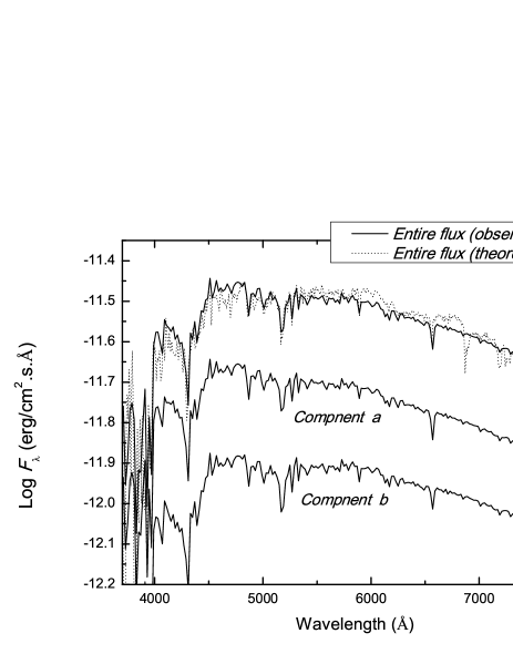
Figure 1: Dotted line: the total observational SED in the continuous spectrum of the system Hip70973. Solid lines: the total computed SED of the two components with $d=38.10\pm 3.04$ pc ($\pi=26.25\pm 1.95$ mas), the computed flux of the primary component with $T_{\rm eff}=5700\pm 75$ K, log $g=4.50\pm 0.05,R=0.98\pm 0.07R_{\odot}$, and the computed flux of the secondary component with $T_{\rm eff}=5400\pm 75$ K, log $g=4.50\pm 0.05,R=0.89\pm 0.07R_{\odot}$.

2.2 Hip72479

For this system we adopted the magnitude difference between the two components $\triangle m=0\hbox{$.\!\!^{m}$}50$ which is the average of all $\triangle m$ measurements under the speckle filters $551nm/22$ (see Table  6) as the closest filters to the visual. This value when used as an input to equation 1, along with the total visual magnitude of the system $m_{v}=8\hbox{$.\!\!^{m}$}534$ from Table 2 as an input to equation 2, results in the preliminary individual $m_{v}$ for each of the component as: $m_{va}=9\hbox{$.\!\!^{m}$}07$ and $m_{vb}=9\hbox{$.\!\!^{m}$}57$.

Following the same procedures explained in the previous section, and using Hipparcos modified parallax measurement as initial input ($\pi=22.59\pm 1.23,d=44.26$pc) as a temporary input for the calculations, the best fit between the total synthetic SED and the observational one taken from Al-Wardat (2002b) was achieved using the following set of parameters (Fig.  2):

$$T_{\rm eff}^{a}=5400\pm 50{\rm K},T_{\rm eff}^{b}=5180\pm 50{\rm K},$$

$$\log g_{a}=4.50\pm 0.05,\log g_{b}=4.60\pm 0.05,$$

$$R_{a}=0.92\pm 0.07R_{\odot}\,\,\textrm{and}\,\,R_{b}=0.84\pm 0.07R_{\odot}.$$

Again here, the values of the estimated radii do not fit exactly those given by Gray (2005), Lang (1992) and the R-L-T relation (equation  4) for the main sequence stars. So, we recalculated the absolute flux using Gray (2005) radii as postulate values leaving the parallax subject to change. Following the guidance of the total observational $V_{J},B_{T},V_{T}$ and $\bigtriangleup m$, the best fit between the synthetic and observational total absolute fluxes was achieved using the following set of parameters

$$T_{\rm eff}^{a}=5400\pm 50{\rm K},T_{\rm eff}^{b}=5180\pm 50{\rm K},$$

$$\log g_{a}=4.50\pm 0.05,\log g_{b}=4.60\pm 0.05,$$

$$R_{a}=0.89\pm 0.07R_{\odot},R_{b}=0.80\pm 0.07R_{\odot},$$

and

$$d=42.40\pm 1.85\,\textrm{pc}(\pi=23.59\pm 1.00\textrm{mas.}),$$

Thus the luminosities follow as: $L_{a}=0.61\pm 0.05L_{\odot}$, and $L_{b}=0.41\pm 0.03L_{\odot}$, with spectral types G9 & K1 for the primary and secondary components respectively.

Table 6: Magnitude difference between the components of the system Hip72479, along with filter used to obtain the observations.

$\triangle m$	filter ($\lambda/\Delta\lambda$)	ref.
$0\hbox{$.\!\!^{m}$}09\pm 0.72$	$V_{Hp}:550nm/40$	1
$1\hbox{$.\!\!^{m}$}00$	$657nm/5$	2
$0\hbox{$.\!\!^{m}$}40$	$551nm/22$	2
$0\hbox{$.\!\!^{m}$}70$	$657nm/5$	2
$0\hbox{$.\!\!^{m}$}60$	$551nm/22$	2

¹ESA (1997), ²Tokovinin et al. (2010).

Figure 2: Dotted line: the total observational SED in the continuous spectrum of the system Hip72479. Solid lines: the total computed SED of the two components with $d=42.40\pm 1.85$ pc. ($\pi=23.59\pm 1.00$ mas), the computed flux of the primary component with $T_{\rm eff}=5400\pm 50$ K, log $g=4.50\pm 0.05,R=0.89\pm 0.07R_{\odot}$, and the computed flux of the secondary component with $T_{\rm eff}=5180\pm 50$ K, log $g=4.60\pm 0.05,R=0.80\pm 0.07R_{\odot}$.

3 Synthetic photometry

In addition to the direct comparison, we can check the reliability of our method of estimating the physical and geometrical parameters by comparing the observed magnitudes of the combined system from different ground or space based telescopes with the synthetic ones. For that, we used the following relation (Maíz Apellániz 2006, 2007):

$$m_{p}[F_{\lambda,s}(\lambda)]=-2.5\log\frac{\int P_{p}(\lambda)F_{\lambda,s}(\lambda)\lambda{\rm d}\lambda}{\int P_{p}(\lambda)F_{\lambda,r}(\lambda)\lambda{\rm d}\lambda}+{\rm ZP}_{p}\,,$$ (8)

to calculate the total and individual synthetic magnitudes of the systems, where $m_{p}$ is the synthetic magnitude of the passband $p$, $P_{p}(\lambda)$ is the dimensionless sensitivity function of the passband $p$, $F_{\lambda,s}(\lambda)$ is the synthetic SED of the object and $F_{\lambda,r}(\lambda)$ is the SED of the reference star (Vega). Zero points (ZP_p) from Maíz Apellániz (2007) (and references there in) were adopted.

The results of the calculated magnitudes and colour indices of the combined system and individual components, in different photometrical systems, are shown in Tables 7 & 8.

Table 7: Magnitudes and colour indices of the synthetic spectra of the system Hip70973.

Sys.	Fil.	total	comp.	comp.
		$\sigma=\pm 0.03$	a	b
Joh-	$U$	8.74	9.17	9.96
Cou.	$B$	8.43	8.92	9.55
	$V$	7.68	8.20	8.73
	$R$	7.28	7.82	8.29
	$U-B$	0.31	0.25	0.41
	$B-V$	0.76	0.72	0.82
	$V-R$	0.41	0.38	0.44
Ström.	$u$	9.88	10.31	11.11
	$v$	8.84	9.30	9.99
	$b$	8.09	8.59	9.17
	$y$	7.65	8.17	8.69
	$u-v$	1.04	1.01	1.12
	$v-b$	0.75	0.71	0.82
	$b-y$	0.45	0.43	0.48
Tycho	$B_{T}$	8.63	9.10	9.77
	$V_{T}$	7.76	8.28	8.82
	$B_{T}-V_{T}$	0.87	0.83	0.95

Table 8: Magnitudes and colour indices of the synthetic spectra of the system Hip72479.

Sys.	Fil.	total	comp.	comp.
		$\sigma=\pm 0.03$	a	b
Joh-	$U$	$9.74$	$10.19$	$10.91$
Cou.	$B$	9.28	9.78	10.36
	$V$	8.43	8.96	9.47
	$R$	7.97	8.52	8.98
	$U-B$	0.46	0.41	0.56
	$B-V$	0.85	0.82	0.89
	$V-R$	0.46	0.44	0.49
Ström.	$u$	10.90	11.34	12.08
	$v$	9.74	10.22	10.86
	$b$	8.88	9.40	9.93
	$y$	8.39	8.92	9.37
	$u-v$	1.15	1.12	1.23
	$v-b$	0.86	0.82	0.92
	$b-y$	0.49	0.48	0.51
Tycho	$B_{T}$	9.51	10.00	10.60
	$V_{T}$	8.52	9.05	9.56
	$B_{T}-V_{T}$	0.98	0.95	1.04

4 Results and discussion

Looking deeply at the achieved best fit between the total synthetic SED’s and the observational ones (Figs.  1 & 2), we see that there is a good overall coincidence in the maximum values of the absolute fluxes and the shape of the continuum except for the blue part of the spectrum around $\lambda 4700\textrm{\AA}$ (Fig. 3). A part of this disagreement is due to the lack of some opacities in the synthetic SED’s and to the difference in the resolution between the synthetic and observational spectra.

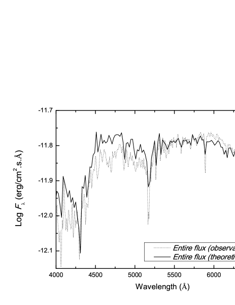
Figure 3: An expanded look at the fit between the total synthetic SED’s and the observational ones for the left part of the spectrum of the system Hip72479.

A comparison between the synthetic magnitudes, colours and magnitude differences with the observational ones (Table 9) shows a very good consistency within the error values. This gives a good indication for the reliability of the estimated parameters of the individual components of the system, which are listed in Tables 10 & 11.

Table 9: Comparison between the observational and synthetic magnitudes, colours and magnitude differences for both systems.

Hip70973.	$\textrm{Obs}.^{*}$	Synth. (this work)
$V_{J}$	$7\hbox{$.\!\!^{m}$}68$	$7\hbox{$.\!\!^{m}$}68\pm 0.03$
$B_{T}$	$8\hbox{$.\!\!^{m}$}667\pm 0.014$	$8\hbox{$.\!\!^{m}$}63\pm 0.03$
$V_{T}$	$7\hbox{$.\!\!^{m}$}781\pm 0.011$	$7\hbox{$.\!\!^{m}$}76\pm 0.03$
$(B-V)_{J}$	$0\hbox{$.\!\!^{m}$}775\pm 0.003$	$0\hbox{$.\!\!^{m}$}76\pm 0.04$
$\triangle m$	$0\hbox{$.\!\!^{m}$}56^{\dagger}$	$0\hbox{$.\!\!^{m}$}53\pm 0.04$
Hip72479
$V_{J}$	$8\hbox{$.\!\!^{m}$}42$	$8\hbox{$.\!\!^{m}$}43\pm 0.03$
$B_{T}$	$9\hbox{$.\!\!^{m}$}540\pm 0.020$	$9\hbox{$.\!\!^{m}$}51\pm 0.03$
$V_{T}$	$8\hbox{$.\!\!^{m}$}534\pm 0.014$	$8\hbox{$.\!\!^{m}$}52\pm 0.03$
$(B-V)_{J}$	$0\hbox{$.\!\!^{m}$}866\pm 0.007$	$0\hbox{$.\!\!^{m}$}85\pm 0.04$
$\triangle m$	$0\hbox{$.\!\!^{m}$}50^{\dagger}$	$0\hbox{$.\!\!^{m}$}51\pm 0.04$

^∗See Table 2.

^†Average value for the filters $550nm/40$ & $551nm/22$ (Tables  4  &  6) .

Concerning the accuracy of our estimated parallaxes, it depends on the accuracy of the input radii as it is clear from equation  6 and  7. This means that the first solution which depends on Hipparcos new parallax is not excluded at all, especially if we know that the values of the radii were higher in the tables of Gray (2005) comparing with tables of Lang (1992).

Fig. 4 shows the positions of the components on the evolutionary tracks of Girardi et al. (2000), where the error bars in the figure include the effect of the parallax uncertainty. The ages of the systems can be established from the evolutionary tracks.

It is clear from the parameters of the system’s components and their positions on the evolutionary tracks that they are solar type main sequence stars, in the early stages of their life. Depending on the formation theories, fragmentation is a possible process for the formation of the systems studied in this work. Where Bonnell (1994) concludes that fragmentation of a rotating disk around an incipient central protostar is possible, as long as there is continuing infall. Zinnecker & Mathieu (2001) pointed out that hierarchical fragmentation during rotational collapse has been invoked to produce binaries and multiple systems.

Figure 4: The systems’ components on the evolutionary tracks (solar abundance) of Girardi et al. (2000).

Table 10: Parameters of the components of the system Hip70973.

Component	a	b
$T_{\rm eff}$ (K)	$5700\pm 75$	$5400\pm 75$
Radius (R⊙)	$0.98\pm 0.07$	$0.89\pm 0.07$
$\log g$	$4.50\pm 0.05$	$4.50\pm 0.05$
$L(L_{\odot})$	$0.91\pm 0.08$	$0.61\pm 0.05$
$M_{v}^{*}$	$4.97\pm 0.10$	$5.77\pm 0.10$
Mass, ($M_{\odot})^{*}$	$1.07\pm 0.08$	$0.94\pm 0.05$
Sp. Type∗	G4	G9
Parallax (mas)	$26.25\pm 1.95$
Age (Gy)	$2.7\pm 0.3$

^∗depending on the tables of Gray (2005).

Table 11: Parameters of the components of the system Hip72479.

Component	a	b
$T_{\rm eff}$ (K)	$5400\pm 50$	$5180\pm 50$
Radius (R⊙)	$0.89\pm 0.07$	$0.80\pm 0.07$
$\log g$	$4.50\pm 0.05$	$4.60\pm 0.05$
$L(L_{\odot})$	$0.61\pm 0.05$	$0.41\pm 0.03$
$M_{v}^{*}$	$5.77\pm 0.10$	$6.25\pm 0.10$
Mass, ($M_{\odot})^{*}$	$0.94\pm 0.05$	$0.85\pm 0.04$
Sp. Type∗	G9	K1
Parallax (mas)	$23.59\pm 1.00$
Age (Gy)	$2.7\pm 0.3$

^∗depending on the tables of Gray (2005).

5 Conclusions

The analysis of the two VCBS, Hip70973 and Hip72479, using atmospheric modelling results in the following main conclusions.

1. The parameters of the systems’ components were estimated depending on the best fit between the observational SED and synthetic ones built using the atmospheric modelling of the individual components.

2. New parallaxes of the systems were estimated from these stellar parameters.

3. From the parameters of the systems’ components and their positions on the evolutionary tracks, we showed that the components within each system are similar solar type main sequence stars (G4 & G9 for Hip70973 and G9 & K1 for Hip72479).

4. The total and individual $UBVR$ Johnson-Cousins, $uvby$ Strömgren and $BV$ Tycho synthetic magnitudes and colours of the systems were calculated.

5. Because of the high similarity of the two components within each system, fragmentation is proposed as the most likely process for the formation and evolution of both systems.

References

- Al-Wardat (2002a) Al-Wardat, M. A. 2002a, Bull. Special Astrophys. Obs., 53, 51
- Al-Wardat (2002b) Al-Wardat, M. A. 2002b, Bull. Special Astrophys. Obs., 53, 58
- Al-Wardat (2007) Al-Wardat, M. A. 2007, Astronomische Nachrichten, 328, 63
- Al-Wardat (2009) Al-Wardat, M. A. 2009, Astronomische Nachrichten, 330, 385
- Al-Wardat & Widyan (2009) Al-Wardat, M. A. & Widyan, H. 2009, Astrophysical Bulletin, 64, 365
- Balega et al. (2002) Balega, I. I., Balega, Y. Y., Hofmann, K.-H., et al. 2002, Astronom. and Astrophys., 385, 87
- Bonnell (1994) Bonnell, I. A. 1994, Monthly Notices Roy. Astronom. Soc., 269, 837
- Couteau (1960) Couteau, P. 1960, Journal des Observateurs, 43, 13
- Docobo et al. (2000) Docobo, J. A., Balega, Y. Y., Ling, J. F., Tamazian, V., & Vasyuk, V. A. 2000, Astronom. J., 119, 2422
- Eggen (1965) Eggen, O. J. 1965, Astronom. J., 70, 19
- Eggen (1967) Eggen, O. J. 1967, Annu. Rev. Astronom. Astrophys., 5, 105
- ESA (1997) ESA. 1997, The Hipparcos and Tycho Catalogues (ESA)
- Girardi et al. (2000) Girardi, L., Bressan, A., Bertelli, G., & Chiosi, C. 2000, Astronom. and Astrophys. Suppl. Ser., 141, 371
- Gray (2005) Gray, D. F. 2005, The Observation and Analysis of Stellar Photospheres, ed. Gray, D. F.
- Heintz (1981) Heintz, W. D. 1981, Astrophys. J. Suppl., 45, 559
- Horch et al. (2008) Horch, E. P., van Altena, W. F., Cyr, Jr., W. M., et al. 2008, Astronom. J., 136, 312
- Lang (1992) Lang, K. R. 1992, Astrophysical Data I. Planets and Stars., ed. K. R. Lang
- Maíz Apellániz (2006) Maíz Apellániz, J. 2006, Astronom. J., 131, 1184
- Maíz Apellániz (2007) Maíz Apellániz, J. 2007, in Astronomical Society of the Pacific Conference Series, Vol. 364, The Future of Photometric, Spectrophotometric and Polarimetric Standardization, ed. C. Sterken, 227–+
- Morel (1970) Morel, P. J. 1970, Astronom. and Astrophys. Suppl. Ser., 1, 115
- Nordström et al. (2004) Nordström, B., Mayor, M., Andersen, J., et al. 2004, Astronom. and Astrophys., 418, 989
- Roberts (2011) Roberts, Jr., L. C. 2011, Monthly Notices Roy. Astronom. Soc., 413, 1200
- Roberts et al. (2005) Roberts, Jr., L. C., Turner, N. H., Bradford, L. W., et al. 2005, Astronom. J., 130, 2262
- Shatskii & Tokovinin (1998) Shatskii, N. I. & Tokovinin, A. A. 1998, Astronomy Letters, 24, 673
- Söderhjelm (1999) Söderhjelm, S. 1999, Astronom. and Astrophys., 341, 121
- Tokovinin et al. (2010) Tokovinin, A., Mason, B. D., & Hartkopf, W. I. 2010, Astronom. J., 139, 743
- van den Bos (1945) van den Bos, W. H. 1945, Monthly Notes of the Astronomical Society of South Africa, 4, 3
- van den Bos (1954) van den Bos, W. H. 1954, Circular of the Union Observatory Johannesburg, 114, 236
- van den Bos (1964) van den Bos, W. H. 1964, Republic Observatory Johannesburg Circular, 123, 62
- van Leeuwen (2007) van Leeuwen, F. 2007, Astronom. and Astrophys., 474, 653
- Zinnecker & Mathieu (2001) Zinnecker, H. & Mathieu, R., eds. 2001, IAU Symposium, Vol. 200, The Formation of Binary Stars