Lie Group Contractions and Relativity Symmetries

Abstract

With a more relaxed perspective on what constitutes a relativity symmetry mathematically, we revisit the notion of possible relativity or kinematic symmetries mutually connected through Lie algebra contractions. We focus on the contractions of an $SO(m,n)$ symmetry as a relativity symmetry on an $m+n$ dimension geometric arena, which generalizes the notion of spacetime, and discuss systematically contractions that reduce the dimension one at a one, aiming at going one step beyond what has been discussed in the literature. Our key results are five different contractions of a Galilean-type symmetry $G(m,n)$ preserving a symmetry of the same type at dimension $m+n-1$, e.g. a $G(m,n-1)$, together with the coset space representations that correspond to the usual physical picture. Most of the results are explicitly illustrated through the example of symmetries obtained from the contraction of $SO(2,4)$, which is the particular case for our interest on the physics side as the proposed relativity symmetry for “quantum spacetime”. The contractions from $G(1,3)$ may be relevant to real physics.

I introduction

In the early 50’s, Inönü-Wigner contraction was introduced to understand the structure between the symmetries for Einstein relativity and its low velocity limit – Galilean relativity IW . The procedure and its generalizations have since been established as a way of obtaining from semisimple Lie groups/algebras interesting nilpotent ones. On the physics side, Lie algebra contraction has been used to study plausible relativity symmetries, most noticeably in Refs.con1 ; con2 . Lie group deformation or stabilization CO is essentially the inverse process of such a contraction . In particular, deformation of Einstein special relativity, or the Poincaré $ISO(1,3)$ symmetry , was introduced as a mean to go beyond Einstein relativity to a new relativity incorporating the quantum scale, as inspired by the early work of Snyder S . This perspective of a Quantum Relativity picture for the ‘quantum spacetime’ is the main idea behind an area of recent research A . The interest in such deformed special relativities was mostly rekindled by a series of papers around the beginning of the century dsr . We depart from most of the other works in the literature by focusing on a simple picture within Lie group/algebra, as advocated in Ref.CO . Two important new ideas are introduce when putting the mathematics into the suggested physics framework. The first one is the linear (coset space) realization picture 023 , like the Minkowski spacetime realization of $ISO(1,3)$ symmetry. The latter, when applied to the new relativity symmetries, dictates the radical idea of the ‘quantum spacetime’ being more than spacetime. One obtains a pseudo-Euclidean space with new coordinates, the physical meaning of which is neither space nor time. Our beginning exploration of the role of such coordinates in physics already shows some interesting results 023 ; 030 ; 036 ; 037 . The second important idea we introduced is that the quantum scale has to be incorporated into the symmetry structure through two parameters instead of just one 030 ; 031 . The two parameters, together with speed of light $c$, essentially give all the fundamental constants one would think relevant to quantum spacetime, namely $c$, the Newton constant $G$, and the quantum $\hbar$.

In Ref.036 , we introduced new relativities called Poincaré-Snyder and Snyder relativities. These are supposed to be intermediate relativities between Einstein relativity and the Quantum Relativity we identified in Ref.030 . We have explored the classical and quantum mechanics of the Poincaré-Snyder relativity of a $G(1,3)$ symmetry, with some success 036 ; 037 . The current study is an out-growth from that work, aiming both to clarify the relation between the mathematics and physics of all the possibly relevant relativity symmetries under the framework. We also explore the somewhat boarder mathematics picture in the interest of generic mathematical physics. The strategy here is to analyze symmetry contractions starting from $SO(m,n)$ with $SO(2,4)$ as the specific one of interest for our physics program.

It is interesting to note that on the mathematical physics side, there has been interesting recent developments on the topic of symmetry (algebra) contractions glc ; gdc ; ck . In particular, Ref.ck provides a nice framework for describing a large set of interesting contractions within the framework of the $SO(m,n)$ symmetries.

In the next section, we discuss our perspective on what may constitute a relativity symmetry, which sets the stage for the Lie algebras we choose to focus on. The perspective represents a plausible modification or enrichment of the concept of relativity symmetry, as compared to the traditional one, as given in the classic 1968 analysis con1 . In Sec.III, we discuss the mathematics of symmetries through applying the contractions. We basically use only the simple contractions of Inönü-Wigner. We will however give some comments on the relation between our results and the other contraction pictures in the appendix. A first look at the physics picture of some plausible relativity symmetries connected to our theme in the Quantum Relativity effort will be discussed in Sec.IV, after which we conclude the paper.

II relativity symmetry

We are interested in group/algebra symmetry which could be the relativity symmetry in physics. That is to say, we are interested in algebras or groups which maybe considered as the isometry of some ‘classical’ geometric arena, such as the familiar three dimensional space or four dimensional spacetime, for the description of fundamental physics. We take a rotation-type $SO(m,n)$ symmetry as a standard, indispensable, part. The rationale behind it is dictated by the physical picture of the isotropic arena having real coordinates. Our Quantum Relativity symmetry is $SO(2,4)$ 030 . $SO(m,n)$ as a semisimple symmetry is stable against deformations. Hence, studying symmetry contractions starting from $SO(m,n)$ is a sensible strategy. The symmetry acts naturally on a $(m+n)$ dimensional classical geometry, or a hypersurface of constant ‘radius’ inside it. Such a geometric realization is what we will stick to in all our considerations of any one of the related mathematical symmetries regarded as a relativity symmetry. We mostly use the phrase ‘dimension of the relativity’ to mean the dimension of such a geometry here. We emphasize again that the physical interpretation of classical geometric fundamental arena should not be restricted to the usual spacetime one.

Usually, we like to consider the arena as admitting also (coordinate) translation symmetries, though our Quantum Relativity is rather a counter example in this respect. A pure $SO(m,n)$ symmetry as a relativity/kinematic symmetry is actually familiar con1 , under the picture of curved ‘spacetime’. There has also been interesting recent developments in some particle dynamics picture of de-Sitter special relativity dssr . With the commuting translations added, that gives rises to an $ISO(m,n)$ symmetry. A further kind of nontrivial symmetry in a relativity is given by the example of the Galilean boosts. We call boosts here all such symmetries characterized by the structure as translations depending on a parameter external to the arena, for instance the Galilean time. The Galilean (velocity) boosts together with the time translation supplemented to an $ISO(0,3)$ gives the Galilei group $G(0,3)$. From the mathematics point of view, the boosts can be defined through the specific commutation relationship between their generators and those of the rotations and translations. In that sense, boosts are boosts only relative to a set of translations and a ‘Hamiltonian’ generator exemplified by the generator of time translation in $G(0,3)$. Hence the so-called Lorentz boosts are no boosts; they are spacetime rotations. Under this framework, we have introduced the $G(1,3)$ symmetry for what we called Poincaré-Snyder relativity 036 ; 037 . The latter as an extension of the familiar $ISO(1,3)$ is a descendant from the $SO(2,4)$ quantum relativity symmetry 030 via contractions through an $ISO(1,4)$. Those symmetries and others connected to them through symmetry algebra contractions are the ones we will discuss in this paper.

The key results of the paper are symmetries obtained from contractions of $G(m,n)$ preserving a subgroup of the same type of dimension $m+n-1$, illustrated by the case of $G(1,3)$, together with the contracted coset space representations corresponding to the usual relativity picture of the Newtonian/Galilean space and Einstein/Minkowski spacetime. The physical picture maybe relevant to nature under the background perspective of our Quantum Relativity framework.

III Relativity Symmetry Contractions from $ISO(m,n)$ and $G(m,n)$.

A generic picture on contractions from $SO(m,n)$ to $ISO(m-1,n)$ or $ISO(m,n-1)$ as well as contractions from $ISO(m,n)$ to $G(m-1,n)$ or $G(m,n-1)$ can be find in Gilmore’s bookG . For an illustration within our perspective, let us sketch the contraction of an $ISO(m,n)$ type symmetry to one of $G(m,n)$ type, using $ISO(1,4)$ to $G(1,3)$ as an explicit example. It starts by picking a subalgebra to be preserved. We have in mind going from a possible relativity symmetry on a $(m+n)$ dimensional geometry to one of a $(m+n-1)$ dimensional geometry. The one dimension ‘removed’ may be taken to be one of time-like ($-$) or space-like (+) geometric signature. We take the latter choice for $ISO(1,4)$ to $G(1,3)$. That means we pick $SO(m,n-1)$, i.e. $SO(1,3)$ in this case, as part of the subalgebra. Unlike the simplest case of contraction from $SO(m,n)$, $SO(m,n-1)$ is not a maximal subalgebra of $ISO(m,n)$. The nonzero commutators among generators of $ISO(1,4)$ can be given as

$$[J_{\mu\nu},J_{\lambda\rho}] = -(\eta_{\nu\lambda}J_{\mu\rho}-\eta_{\mu\lambda}J_{\nu\rho}+\eta_{\mu\rho}J_{\nu\lambda}-\eta_{\nu\rho}J_{\mu\lambda})\;,$$ (1)

$$[J_{\mu\nu},J_{{\scriptscriptstyle 4}\rho}]=-(\eta_{\nu\rho}J_{{\scriptscriptstyle 4}\mu}-\eta_{\mu\rho}J_{{\scriptscriptstyle 4}\nu})\;,$$

$$[J_{\mu\nu},P_{\rho}]=-(\eta_{\nu\rho}P_{\mu}-\eta_{\mu\rho}P_{\nu})\;,$$

$$[P_{\scriptscriptstyle 4},J_{{\scriptscriptstyle 4}\mu}]=-P_{\mu}\;,$$

$$[P_{\mu},J_{{\scriptscriptstyle 4}\nu}]=\eta_{\mu\nu}P_{\scriptscriptstyle 4}\;,$$

$$[J_{{\scriptscriptstyle 4}\mu},J_{{\scriptscriptstyle 4}\nu}]=J_{\mu\nu}\;,$$

where the index $4$ denotes the dimension with space-like geometric signature that is singled out. We then take $J_{{\scriptscriptstyle 4}\mu}$ to be among the generators to go through the algebra transformation the singular limit of which gives the contraction. The set of $J_{\mu\nu}$ gives the preserved $SO(1,3)$ symmetry. To keep the resulting symmetry as a $1+3$ dimensional relativity symmetry, the $P_{\mu}$ generators obviously have to be treated in the same way. If we take $P_{\scriptscriptstyle 4}$ with $J_{\mu\nu}$ and redefine the generators by the one parameter transformation

Table 1: A schematic presentation of possible $1+3$ dimensional relativity symmetries from contractions of $ISO(1,4)$. For each case, we listed the generators to be transformed, i.e. taken through the singular limit of a transformation as illustrated in Eq.(2). In the contracted symmetries, the $J_{{\scriptscriptstyle 4}\mu}$ or rather the $K^{\prime}_{\mu}$ generators can be taken as a kind of boosts, or translations dependent on an extra parameter and the $P_{\scriptscriptstyle 4}$ generator is translation in the parameter, in the picture of $G(1,3)$. The extra parameter can be taken as an ‘evolution’ parameter with $P_{\scriptscriptstyle 4}$ corresponding to the ‘Hamiltonian’ of the ‘evolution’ in a canonical formulation 037 . Mathematically as defined in the text, $K^{\prime}_{\mu}$ are boost generators in relation to the translations $P_{\mu}$ and the other generators in $G(1,3)$. There are no boosts in $S(1,3)$ and $S(1,3)$. At the upper level of say $SO(2,4)$, all five $P_{\scriptscriptstyle A}$ will be $J_{5{\scriptscriptstyle\!A}}$ with the standard nonzero commutators among them. Note that all three cases have the same $ISO(1,3)$ subalgebra, $J_{\mu\nu}$ and $P_{\mu}$ part, inside the resulting algebra.

		Contracted Symmetries
	$ISO(1,4)$	$G(1,3)$	$C(1,3)$	$S(1,3)$
$[J_{\mu\nu},J_{\lambda\rho}]=$	$J_{\mu\lambda}$	$J_{\mu\lambda}$	$J_{\mu\lambda}$	$J_{\mu\lambda}$
$[J_{\mu\nu},J_{{\scriptscriptstyle 4}\mu}]=$	$J_{{\scriptscriptstyle 4}\nu}$	$J_{{\scriptscriptstyle 4}\nu}=\bar{\kappa}K^{\prime}_{\nu}$	$J_{{\scriptscriptstyle 4}\nu}=\bar{\kappa}K^{\prime}_{\nu}$	$J_{{\scriptscriptstyle 4}\nu}=\bar{\kappa}K^{\prime}_{\nu}$	$[J_{\mu\nu},K^{\prime}_{\mu}]=K^{\prime}_{\nu}$
$[J_{\mu\nu},P_{\mu}]=$	$P_{\nu}$	$P_{\nu}=\bar{\kappa}P^{\prime}_{\nu}$	$P_{\nu}$	$P_{\nu}=\bar{\kappa}P^{\prime}_{\nu}$	$[J_{\mu\nu},P^{\prime}_{\mu}]=P^{\prime}_{\nu}$
$[J_{{\scriptscriptstyle 4}\mu},P_{\scriptscriptstyle 4}]=$	$P_{\mu}$	$P_{\mu}=\bar{\kappa}P^{\prime}_{\mu}$	0	0	$[K^{\prime}_{\mu},P_{\scriptscriptstyle 4}]=P^{\prime}_{\mu}$
$[J_{{\scriptscriptstyle 4}\mu},P_{\mu}]=$	$P_{\scriptscriptstyle 4}$	0	$P_{\scriptscriptstyle 4}=\bar{\kappa}P^{\prime}_{\scriptscriptstyle 4}$	0	$[K^{\prime}_{\mu},P_{\mu}]=P^{\prime}_{\scriptscriptstyle 4}$
$[J_{{\scriptscriptstyle 4}\mu},J_{{\scriptscriptstyle 4}\nu}]=$	$J_{\mu\nu}$	0	0	0
	generators transformed	$J_{{\scriptscriptstyle 4}\mu},P_{\mu}$	$J_{{\scriptscriptstyle 4}\mu},P_{\scriptscriptstyle 4}$	$J_{{\scriptscriptstyle 4}\mu},P_{\mu},P_{\scriptscriptstyle 4}$

 

$$\left(\begin{array}[]{c}J_{\mu\nu}\\ P_{\scriptscriptstyle 4}\\ K^{\prime}_{\mu}\\ P^{\prime}_{\mu}\\ \end{array}\right):=\left(\begin{array}[]{cccc}I&0&0&0\\ 0&I&0&0\\ 0&0&\frac{1}{{\bar{\kappa}}}I&0\\ 0&0&0&\frac{1}{{\bar{\kappa}}}I\end{array}\right)\left(\begin{array}[]{c}J_{\mu\nu}\\ P_{\scriptscriptstyle 4}\\ J_{{\scriptscriptstyle 4}\mu}\\ P_{\mu}\end{array}\right)\;,$$ (2)

the singular limit of ${\bar{\kappa}}\rightarrow\infty$ gives the $G(1,3)$ algebra. The latter as a relativity symmetry was introduced together with a physical picture in Refs.036 ; 037 . The parameter ${\bar{\kappa}}$ will be a physical constant with a similar role to $c$, the speed of light.

In the place of $P_{\scriptscriptstyle 4}$, one may choose the $P_{\mu}$ or simply nothing to be included into the subalgebra with $J_{\mu\nu}$. In each case taking the rest with $J_{{\scriptscriptstyle 4}\mu}$ through the singular transformation gives a contraction. It is easy to see that the resulting symmetries are $C(1,3)$ and $S(1,3)$, respectively, as given in Table 1. The table only presents a schematic form of the commutators among the generators but should be enough to illustrate the algebras. A contraction simply keeps some commutators unchanged while trivializing some others as shown. The scheme obviously works for any $(m,n)$. Similarly, contractions from $ISO(m,n)$ keeping $SO(m-1,n)$, that is ‘removing’ a dimension of time-like geometric signature, gives rise to $G(m-1,n)$, $C(m-1,n)$, and $S(m-1,n)$. The $G(0,3)$, $C(0,3)$, and $S(0,3)$ relativities are the Galilean, Carroll, and static relativities in the literature (for example, Refs.con1 ; con2 ). Our notation of $C(m,n)$, and $S(m,n)$ follows from there.

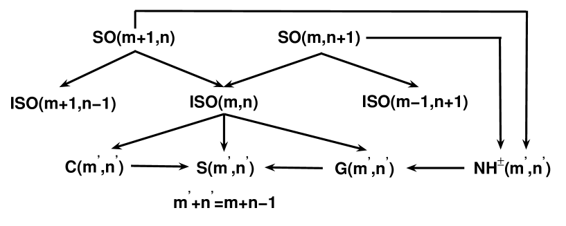
Figure 1: An illustration of some of the contraction paths relating some relativity symmetries of difference up to two in dimensions.

 

The scheme above can be taken to define $G(m,n)$, $C(m,n)$, and $S(m,n)$ symmetries on any $(m+n)$ dimensional geometry. It is also easy to see simple contractions from $G(m,n)$ or $C(m,n)$ to $S(m,n)$ at the same dimension. For our illustrative case in the $ISO(1,4)$ notation, the latter are achieved by taking $J_{{\scriptscriptstyle 4}\mu}$ and $P_{\scriptscriptstyle 4}$ through another singular transformation in the first case, and $J_{{\scriptscriptstyle 4}\mu}$ and $P_{\mu}$ in the second. We illustrate the above contraction paths connecting the symmetries in Fig.1.

We note in passing that if one consider contractions reducing the dimension by two directly, it is possible to get a symmetry beyond what one can get by taking a two step contraction each reducing the dimension by one. An interesting example is given by the $N^{+}(0,3)$ Newton-Hooke case from $SO(1,4)$ con1 ; con2 by-passing $ISO(1,3)$. To match the structure of the analogous $N^{+}(1,3)$ versus those in Table 1, it has the same commutator set as $G(1,3)$ with an extra nonzero $[P_{\mu},P_{\scriptscriptstyle 4}]$. Using $P_{\scriptscriptstyle 4}$, which is $J_{\scriptscriptstyle 54}$ at the $SO(2,4)$ level, gives $[P_{\mu},P_{\scriptscriptstyle 4}]=J_{{\scriptscriptstyle 4}\mu}$, i.e. the commutator of the translations with the Hamiltonian gives the corresponding boost generators. So, the mathematical role of $P_{\mu}$ and $J_{{\scriptscriptstyle 4}\mu}$ are actually symmetrical in $N^{+}(1,3)$. They are both symmetries of the translation type mathematically. The subalgebra generated by $J_{\scriptscriptstyle 54}$ ($P_{\scriptscriptstyle 4}$) and $J_{\mu\nu}$ is preserved when contracting from $SO(2,4)$ directly, i.e. the generators taken through the singular transformations are $J_{5\mu}$ ($P_{\mu}$) and $J_{{\scriptscriptstyle 4}\mu}$. Note that taking out only $P_{\mu}$($J_{5\mu}$) without $P_{\scriptscriptstyle 4}$ ($J_{5\!4}$) and $J_{{\scriptscriptstyle 4}\mu}$ does not leave a closed subalgebra. Similarly, one can project getting $N^{+}(m^{\prime},n^{\prime})$ symmetries from contractions of an $SO(m,n)$ with $m+n=m^{\prime}+n^{\prime}+2$. And it can be further contracted to $G(m^{\prime},n^{\prime})$ or $S(m^{\prime},n^{\prime})$ at the same dimension (see also Fig.1), by again taking $J_{{\scriptscriptstyle 4}\mu}$ and $P_{\scriptscriptstyle 4}$, or $J_{{\scriptscriptstyle 4}\mu}$, $P_{\scriptscriptstyle 4}$, and $P_{\mu}$ through another singular transformation, respectively, in our illustrative case for instance. It can be seen easily that the $SO(m,n)$ can also be directly contracted to an $S(m^{\prime},n^{\prime})$ with $m+n=m^{\prime}+n^{\prime}+2$, but not $G(m^{\prime},n^{\prime})$ or $C(m^{\prime},n^{\prime})$.

Next, we look at contractions from the $G(m,n)$, reducing the dimension by one. This could be useful, for example, in thinking about the low-velocity limit of the Poincaré-Snyder $G(1,3)$ relativity we studied in Refs.036 ; 037 . We will explore that physical picture in the next section. Here, we use $G(1,3)$ for an explicit illustrations of some the mathematics for contraction from a $G(m,n)$, focusing of reducing to a symmetry on a geometry of one less dimension with $G(m-1,n)$ or $G(m,n-1)$ to be preserved. This is to maintain similar features in the contraction sequence from the types of algebras $SO(m,n)$ to $ISO(m,n)$ to $G(m,n)$. In particular, we preserve the $G(0,3)$ subalgebra in our example.

The (nonzero) commutators of $G(m,n)$ are given explicitly here in the notation with boosts $K^{\prime}_{\mu}$ and ‘Hamiltonian’ $H^{\prime}\equiv P_{\scriptscriptstyle 4}$, splitting the time-like dimension from the three space-like ones :

$$[J_{ij},J_{kl}]=-(\eta_{jk}J_{il}-\eta_{ik}J_{jl}+\eta_{il}J_{jk}-\eta_{jl}J_{ik})\;,$$

$$[J_{ij},J_{{\scriptscriptstyle 0}k}]=-(\eta_{jk}J_{{\scriptscriptstyle 0}i}-\eta_{ik}J_{{\scriptscriptstyle 0}j})\;,\qquad[J_{{\scriptscriptstyle 0}i},J_{{\scriptscriptstyle 0}j}]=-J_{ij}\;,$$

$$[J_{ij},P^{\prime}_{k}]=-(\eta_{jk}P^{\prime}_{i}-\eta_{ik}P^{\prime}_{j})\;,$$

$$[J_{{\scriptscriptstyle 0}i},P^{\prime}_{\scriptscriptstyle 0}]=-P^{\prime}_{i}\;,\qquad[J_{{\scriptscriptstyle 0}i},P^{\prime}_{i}]=-P^{\prime}_{\scriptscriptstyle 0}\;,$$

$$[J_{ij},K^{\prime}_{k}]=-(\eta_{jk}K^{\prime}_{i}-\eta_{ik}K^{\prime}_{j})\;,$$

$$[J_{{\scriptscriptstyle 0}i},K^{\prime}_{\scriptscriptstyle 0}]=-K^{\prime}_{i}\;,\qquad[J_{{\scriptscriptstyle 0}i},K^{\prime}_{i}]=-K^{\prime}_{\scriptscriptstyle 0}\;,$$

$$[H^{\prime},K^{\prime}_{\scriptscriptstyle 0}]=-P^{\prime}_{\scriptscriptstyle 0}\;,\qquad[H^{\prime},K^{\prime}_{i}]=-P^{\prime}_{i}\;.$$ (3)

Denote the subalgebra to be preserved in the contraction process by ${h}$ and the complementary vector-subspace ${p}$. Recall that generators of ${p}$ are to be taken to the limit of the singular transformation. Our first task is to look at choices of the ${h}$ and ${p}$ splitting. The $J_{ij}$ generators of the $SO(0,3)$ subalgebra is certainly what we want to keep in going from $1+3$ dimension to $0+3$ dimension. Notice that inside the $G(1,3)$, there is an $ISO(1,3)$ subalgebra. From the above analysis, we can see that among the generators of the latter, keeping $P^{\prime}_{\scriptscriptstyle 0}$ or $P^{\prime}_{i}$ or nothing together with the $J_{ij}$ will contract the $ISO(1,3)$ to $G(0,3)$, $C(0,3)$, or $S(0,3)$, respectively. As said, we stick here to the case getting $G(0,3)$. Keeping $P^{\prime}_{\scriptscriptstyle 0}$ with $J_{ij}$ as the minimal set of generators for ${h}$ and $J_{{\scriptscriptstyle 0}i}$ and $P^{\prime}_{i}$ in ${p}$, one can see that there are six possible choices of the ${h}$ and ${p}$ splitting, as follows:

$$\begin{array}[]{c|lrcc}\mbox{Case}&\lx@intercol\hfil\mbox{\boldmath${h}$}\hfil\lx@intercol&\lx@intercol\hfil\mbox{\boldmath${p}$}\hfil\lx@intercol\\ \hline\cr A&{\ J_{ij},P^{\prime}_{\scriptscriptstyle 0}}&{H^{\prime},K^{\prime}_{\scriptscriptstyle 0},K^{\prime}_{i},P^{\prime}_{i},J_{{\scriptscriptstyle 0}i}}&\rightarrow&{H^{\prime\prime},K^{\prime\prime}_{\scriptscriptstyle 0},K^{\prime\prime}_{i},P_{i},K_{i}}\\ B&{\ J_{ij},P^{\prime}_{\scriptscriptstyle 0},H^{\prime}}&{K^{\prime}_{\scriptscriptstyle 0},K^{\prime}_{i},P^{\prime}_{i},J_{{\scriptscriptstyle 0}i}}&\rightarrow&{K^{\prime\prime}_{\scriptscriptstyle 0},K^{\prime\prime}_{i},P_{i},K_{i}}\\ C&{\ J_{ij},P^{\prime}_{\scriptscriptstyle 0},K^{\prime}_{\scriptscriptstyle 0}}&{H^{\prime},K^{\prime}_{i},P^{\prime}_{i},J_{{\scriptscriptstyle 0}i}}&\rightarrow&{H^{\prime\prime},K^{\prime\prime}_{i},P_{i},K_{i}}\\ D&{\ J_{ij},P^{\prime}_{\scriptscriptstyle 0},H^{\prime},K^{\prime}_{\scriptscriptstyle 0}}&{K^{\prime}_{i},P^{\prime}_{i},J_{{\scriptscriptstyle 0}i}}&\rightarrow&{K^{\prime\prime}_{i},P_{i},K_{i}}\\ E&{\ J_{ij},P^{\prime}_{\scriptscriptstyle 0},K^{\prime}_{i}}&{H^{\prime},K^{\prime}_{\scriptscriptstyle 0},P^{\prime}_{i},J_{{\scriptscriptstyle 0}i}}&\rightarrow&{H^{\prime\prime},K^{\prime\prime}_{\scriptscriptstyle 0},P_{i},K_{i}}\\ F&{\ J_{ij},P^{\prime}_{\scriptscriptstyle 0},K^{\prime}_{\scriptscriptstyle 0},K^{\prime}_{i}}&{H^{\prime},P^{\prime}_{i},J_{{\scriptscriptstyle 0}i}}&\rightarrow&{H^{\prime\prime},P_{i},K_{i}}\end{array}$$

where the new set of generators in ${p}$ are given by the original set times ${1}/{c}$ with the singular limit $c\to\infty$. We skip the tedious mathematical details and give a schematic presentation of the results in Table 2. The cases A to F, as defined above are listed, with the resulting symmetries given the names or notations shown which are to be explained in the discussion below. The $(3)$ as in $G_{X}(3)$ for all cases is a suppressed form for $(0,3)$, indicating the $SO(0,3)$ subalgebra. A similar analysis applying to $G(m,n)$ with the condition that a lower dimensional $C(m,n)$ or $S(m,n)$, instead of $G(m,n)$, being the subalgebra to be preserved, can certainly be performed to yield further alternatives.

Table 2: A schematic presentation of possible $0+3$ dimensional relativity symmetries from the contraction of $G(1,3)$. Having the Galilean symmetry $G(3)$ [$\equiv G(0,3)$] as a subgroup is taken as a criterion. The six different results of symmetry contractions follow from the discussion in the text. As in the case of Table 1, new generators like $K_{i}$, $P_{i}$, $K^{\prime\prime}_{i}$, … etc. shown in the last columns are to be used in the contracted symmetries. $P^{\prime}_{\scriptscriptstyle 0}$ is to be renamed as $H$.

	Poincaré-Snyder	F	E	D	C	B	A	Galilean
	$G(1,3)$	$G_{B}(3)$	$G_{C}(3)$	$G_{D}(3)$	$G_{T}(3)$	$G_{B}(3)$	$G_{S}(3)$	$G(3)$
$[J_{ij},J_{kl}]=$	$J_{ik}$	$J_{ik}$	$J_{ik}$	$J_{ik}$	$J_{ik}$	$J_{ik}$	$J_{ik}$	$J_{ik}$
$[J_{ij},J_{{\scriptscriptstyle 0}i}]=$	$J_{{\scriptscriptstyle 0}j}$	$J_{{\scriptscriptstyle 0}j}$	$J_{{\scriptscriptstyle 0}j}$	$J_{{\scriptscriptstyle 0}j}$	$J_{{\scriptscriptstyle 0}j}$	$J_{{\scriptscriptstyle 0}j}$	$J_{{\scriptscriptstyle 0}j}$	$[J_{ij},K_{i}]=K_{j}$	$K_{j}=\frac{1}{c}J_{{\scriptscriptstyle 0}j}$
$[J_{ij},P^{\prime}_{i}]=$	$P^{\prime}_{j}$	$P^{\prime}_{j}$	$P^{\prime}_{j}$	$P^{\prime}_{j}$	$P^{\prime}_{j}$	$P^{\prime}_{j}$	$P^{\prime}_{j}$	$[J_{ij},P_{i}]=P_{j}$	$P_{j}=\frac{1}{c}P^{\prime}_{j}$
$[J_{{\scriptscriptstyle 0}i},P^{\prime}_{\scriptscriptstyle 0}]=$	$-P^{\prime}_{i}$	$-P^{\prime}_{i}$	$-P^{\prime}_{i}$	$-P^{\prime}_{i}$	$-P^{\prime}_{i}$	-$P^{\prime}_{i}$	$-P^{\prime}_{i}$	$[K_{i},H]=P_{i}$	$H=P^{\prime}_{\scriptscriptstyle 0}$
$[J_{{\scriptscriptstyle 0}i},J_{{\scriptscriptstyle 0}j}]=$	$-J_{ij}$	0	0	0	0	0	0	$[K_{i},K_{j}]=0$
$[J_{{\scriptscriptstyle 0}i},P^{\prime}_{i}]=$	$-P^{\prime}_{\scriptscriptstyle 0}$	0	0	0	0	0	0	$[K_{i},P_{j}]=0$
$[J_{ij},K^{\prime}_{i}]=$	$K^{\prime}_{j}$	$K^{\prime}_{j}$	$K^{\prime}_{j}$	$K^{\prime}_{j}$	$K^{\prime}_{j}$	$K^{\prime}_{j}$	$K^{\prime}_{j}$	$[J_{ij},K^{\prime\prime}_{i}]=K^{\prime\prime}_{j}$, $K^{\prime\prime}_{i}=\frac{1}{c}K^{\prime}_{i}$
		($K^{\prime\prime}_{\scriptscriptstyle 0}=\frac{1}{c}K^{\prime}_{\scriptscriptstyle 0}$ for A, B, E )						for A, B, C, D
$[J_{{\scriptscriptstyle 0}i},K^{\prime}_{i}]=$	$-K^{\prime}_{\scriptscriptstyle 0}$	0	$-K^{\prime}_{\scriptscriptstyle 0}$	0	0	0	0	$[K_{i},K^{\prime}_{i}]=-K^{\prime\prime}_{\scriptscriptstyle 0}$ for E
$[J_{{\scriptscriptstyle 0}i},K^{\prime}_{\scriptscriptstyle 0}]=$	$-K^{\prime}_{i}$	0	0	$-K^{\prime}_{i}$	$-K^{\prime}_{i}$	0	0	$[K_{i},-K^{\prime}_{\scriptscriptstyle 0}]=K^{\prime\prime}_{i}$ for C, D
$[K^{\prime}_{i},H^{\prime}]=$	$P^{\prime}_{i}$	$P^{\prime}_{i}$	$P^{\prime}_{i}$	$P^{\prime}_{i}$	0	$P^{\prime}_{i}$	0	$[K^{\prime\prime}_{i},H^{\prime}]=P_{i}$ for B, D
		($H^{\prime\prime}=\frac{1}{c}H^{\prime}$ for A, C, E, F )						$[K^{\prime}_{i},H^{\prime\prime}]=P_{i}$ for E, F
$[K^{\prime}_{\scriptscriptstyle 0},H^{\prime}]=$	$P^{\prime}_{\scriptscriptstyle 0}$	0	0	$P^{\prime}_{\scriptscriptstyle 0}$	0	0	0	$[K^{\prime}_{\scriptscriptstyle 0},H^{\prime}]=H$ for D

 

The important set of extra generators all the new symmetries have, apart from the $G(0,3)$ subalgebra, is the $K^{\prime}_{i}$ or $K^{\prime\prime}_{i}$. The latter transform as components of a vector on the three dimensional space on which we have the $SO(0,3)$ rotations, similar to the $K_{i}$ and $P_{i}$ vectors. They commute with the $P_{i}$ translations in all cases, and commute also with the $K_{i}$ velocity boosts in all except case E. For case A there is no further extra nonzero commutator. So apart from the $[K_{i},H]=P_{i}$ required in $G(0,3)$, it has a structure similar to the static symmetry $S(0,3)$. Hence we named it $G_{S}(0,3)$. This simple structure may have little to offer in a physics picture. We can see that the $K^{\prime\prime}_{i}$ for cases B and D maintain the full algebraic structure of a kind certaun of boosts on the 3D space with $H^{\prime}$ as the corresponding ‘Hamiltonian’, i.e. we have $[K^{\prime\prime}_{i},H^{\prime}]=P_{i}$. Case F is similar, with the ‘Hamiltonian’ being $H^{\prime\prime}$ and it has $K^{\prime}_{i}$ instead of $K^{\prime\prime}_{i}$. Actually, case F yields an algebra isomorphic to that of case B. Case D differs from the latter in having two more nonzero commutators : $[K_{i},-K^{\prime}_{\scriptscriptstyle 0}]=K^{\prime\prime}_{i}$ and $[K^{\prime}_{\scriptscriptstyle 0},H^{\prime}]=H$. The former shows a relation between $K_{i}$ and $K^{\prime\prime}_{i}$ similar to that between $K_{i}$ and $P_{i}$ with the role of $-K^{\prime}_{\scriptscriptstyle 0}$ to be matched to that of $H$. So the $K^{\prime\prime}_{i}$ are translations relative to the boosts $K_{i}$ and boosts relative to the translations $P_{i}$. The structure is quite complicated, somewhat like having a type of double layer Galilean structure among $K_{i}$, $K^{\prime\prime}_{i}$, and $P_{i}$. We denote the case B (and hence also F) algebra by $G_{B}(0,3)$ for having an extra set of boosts, and that for case D as $G_{D}(0,3)$ for the sort of double Galilean structure. $G_{D}(0,3)$ is the one with the most complicated structure among all cases. However, it happens to be the only one obtainable in a $Z_{2}^{\otimes\scriptscriptstyle N}$-graded contraction framework ck which includes all Cayley-Klein symmetries ckm . From that mathematical point of view, it looks like a natural candidate in the sequence :

$$SO(2,4)\;\;\rightarrow\;\;ISO(1,4)\;\;\rightarrow\;\;G(1,3)\;\;\rightarrow\;\;G_{D}(0,3)\;.$$

More details on that aspect we leave to the appendix.

For the remaining two cases, the $K^{\prime}_{i}$ or $K^{\prime\prime}_{i}$ vector does not behave like a set of boosts in terms of its relationship to any translation vector like $P_{i}$. Case C has $[K_{i},-K^{\prime}_{\scriptscriptstyle 0}]=K^{\prime\prime}_{i}$ as the only nonzero commutation relation beyond $J_{ij}$ and the three vector sets. So it has the $K^{\prime\prime}_{i}$ vector behaving like the translations $P_{i}$, with the role of $-K^{\prime}_{\scriptscriptstyle 0}$ being matched to that of $H$ hence like another ‘Hamiltonian’. The algebra has an extra set of translations, hence it is denoted by $G_{T}(0,3)$. Finally, we look at case E. The special commutation relation $[K_{i},K^{\prime}_{i}]=-K^{\prime\prime}_{\scriptscriptstyle 0}$ may remind one of the nonzero commutator between the two vector sets of generators as in the $C(m,n)$ case (see table 1). Recall that $K^{\prime}_{i}$ in this case behave like boosts with respect to $P_{i}$, in contrast to its behaving like translations in $C(0,3)$ with respect to $K_{i}$. We denote it by $G_{C}(0,3)$. In fact, we expect the symmetry to be accessible via a contraction from $C(1,3)$.

The above description of contractions from $G(1,3)$ to the various three dimensional relativity symmetries can obviously be generalized to all the cases of any $G(m,n)$ giving the five new symmetries as $m+n-1$ dimensional relativity symmetries with a $G(m-1,n)$ and $G(m,n-1)$ subgroup.

In the above, though we have been using the terms translations and boosts, they refer only to the algebraic structure — commutation relations with other generators. The only geometric picture we stick to is that of $SO(m,n)$ as rotations. In the next section, we look into some of the exact physics pictures.

IV Realization on the geometric arena

As said, we think about a relativity symmetry as one that is the symmetry of a classical geometric arena similar to but possibly beyond space(time), or reference frame transformations thereof. Here we discuss the plausible geometric picture of some of the new relativity symmetries introduced above. We are interested on the physics side of the contraction pictures motivated by Refs.023 ; 030 . The $SO(2,4)$ Quantum Relativity is formulated as a rotational type isometry on a classical six-geometry with two non-spacetime coordinates ($u$-coordinates) 030 , giving a sort of description of a four dimensional noncommutative spacetime. The relevant part of the six-geometry is only a five dimensional hypersurface satisfying a constraint – a ‘space-like AdS₅’. Some description of the geometric picture has been given without any explicit dynamical notion in the paper.

For the $ISO(1,4)$, named Snyder Relativity in Ref.036 , a quite standard geometric picture of rotations and translations on a (classical) five-geometry with the fifth coordinate being a $u$-coordinate has been adopted. It is a five dimensional (geometric) space of Minkowski type with the coordinate $x^{\scriptscriptstyle 4}$ supplemented to the familiar Minkowski space $M^{4}$ of Einstein spacetime, mathematically it is the natural coset space

$$M^{5}=ISO(1,4)/SO(1,4)\;.$$

This fifth coordinate in the physics picture is to be written as $x^{\scriptscriptstyle 4}=\bar{\kappa}\sigma$ with $\bar{\kappa}$ being essentially the parameter to be used in a further contraction from $ISO(1,4)$, as given in Eqn.(2). The $\bar{\kappa}$ parameter is an imposed invariant momentum, in the spirit of SnyderS essentially adopted from Ref.dsr (see Refs.023 ; 030 ). It assumes the physical dimension of momentum. A further contraction gives the $G(1,3)$ Poincaré-Snyder Relativity 036 ; 037 , which contains the familiar Poincaré symmetry of $ISO(1,3)$ as a preserved subgroup. The process splits out $x^{\scriptscriptstyle 4}$ from the remaining four spacetime coordinates, casting $\sigma$ as an external (absolute) parameter, similar mathematically to the Galilean time. It has, however, the physical dimension of $\frac{time}{mass}$, The original $SO(1,4)$ subgroup is contracted to another $ISO(1,3)$ subgroup of $G(1,3)$, which contains an extra set of boost generators — boosts in relation to the Poincaré translations and a new ‘Hamiltonian’ generator ($K^{\prime}_{\mu}$, $P^{\prime}_{\mu}$, and $P^{\prime}_{\scriptscriptstyle 4}$ of table 1, respectively). The set of four generators transform as a vector in relation to the $3+1$ dimensional rotation $SO(1,3)\subset G(1,3)$, and the transformations they generate, are called momentum boosts . The contraction reduces the coset space $M^{5}=ISO(1,4)/SO(1,4)$ to

$$M^{4}\times I\!\!R=G(1,3)/ISO(1,3)\;,$$

with the $ISO(1,3)$ factored out being the one with the momentum boosts. The $M^{4}$ in the new coset space can be identified as the usual Minkowski spacetime while $I\!\!R$ denotes a line of $\sigma$ values. The above is just the analog of the spacetime picture in the contraction of Einstein Relativity of $ISO(1,3)$ to the Galilean Relativity of $G(0,3)$. Explicitly, we have the $G(1,3)$ realization as given by

$$x^{\prime\mu}={\Lambda^{\mu}}_{\!\nu}x^{\nu}+p^{\mu}\sigma+A^{\mu}\;,$$

$$\sigma^{\prime}=\sigma+S\;,$$ (4)

where ${\Lambda^{\mu}}_{\!\nu}$ is the Lorentz transformation and the $+p^{\mu}\sigma$ part the momentum boosts with the Poincaré-Snyder momentum given by $p^{\mu}=dx^{\mu}/d\sigma$. The picture of the $G(1,3)$ realization can be taken to formulate a canonical realization PP as in Hamiltonian mechanics 037 or a projective representation gq as in quantum mechanics 036 , which are the standard particle dynamic formulations for the corresponding Galilean case. The success of such analyzes suggests the validity of the picture. The phase space Hamiltonian mechanics picture has $\sigma$ as a formal evolution parameter, generated by the $\sigma$-Hamiltonian $H^{\prime}$. It is easy to see the single particle phase space is just the eight dimensional coset space

$$G(1,3)/[SO(1,3)\times T_{\scriptscriptstyle H^{\prime}}]\;,$$

where $T_{\scriptscriptstyle H^{\prime}}$ is the subgroup of $\sigma$-translation generated by $H^{\prime}$. The natural canonical pair of phase space coordinates are $(x^{\mu},p_{\mu})$.

Next, we want to follow the picture and see what happens with further contractions of $G(1,3)$ to the new three dimensional relativity symmetries we described above, or as listed in Table 2. In all these symmetries as contractions from $G(1,3)$ we keep the Poincaré $ISO(1,3)$ subgroup of the spacetime part contracted to $G(0,3)$ as the usual Galilean symmetry. The contraction has a structure similar to that of Eqn.(2), with the index 0 instead of 4 being singled-out from $J_{\mu\nu}$ and $P_{\mu}$ giving the rotations $J_{ij}$ and translations $P^{\prime}_{i}$. The contraction transformation involves the invariant speed $c$ and gives $K_{i}=\frac{1}{c}J_{{\scriptscriptstyle 0}i}$ and $P_{i}=\frac{1}{c}P^{\prime}_{i}$ [$P_{i}$ here is not to be identified exactly as parts of the $P_{\mu}$ of Eqn.(1)]. The generator $P^{\prime}_{\scriptscriptstyle 0}$ in the preserved subalgebra for all cases of Table (2) becomes the usual Hamiltonian that describes time evolution, as the time $t$ from $x^{\scriptscriptstyle 0}=c\,t$ splits off as another external parameter to the remaining three dimensional space. Naively, we have an arena as $I\!\!R^{3}\times I\!\!R\times I\!\!R$ described by $(x^{i},t,\sigma)$.

To start on a firm footing, we go back to the Newtonian space-time coset representation of $G(0,3)$ as given by

$$x^{\prime i}={R^{i}}_{j}x^{j}+V^{i}t+A^{i}\;,$$

$$t^{\prime}=t+B\;.$$ (5)

For a generic element of the corresponding algebra, an infinitesimal transformation, we have

$$\left(\begin{array}[]{c}dt\\ dx^{i}\\ 0\end{array}\right)=\left(\begin{array}[]{ccc}{0}&{0}&b\\ v^{i}&\omega^{i}_{j}&a^{i}\\ {0}&{0}&{0}\end{array}\right)\left(\begin{array}[]{c}t\\ x^{j}\\ 1\end{array}\right)=\left(\begin{array}[]{c}b\\ \omega^{i}_{j}x^{j}+v^{i}t+a^{i}\\ 0\end{array}\right)\;,$$ (6)

where $\omega^{i}_{j},v^{i},a^{i},b$ denotes the set of (infinitesimal) parameters to be exponentiated to describe the group manifold. The matching matrix representation of an infinitesimal transformation the Poincaré $ISO(1,3)$ symmetry is given by

$$\left(\begin{array}[]{c}cdt\\ dx^{i}\\ 0\end{array}\right)=\left(\begin{array}[]{ccc}0&\beta_{j}&b\\ \beta^{i}&\omega^{i}_{j}&a^{i}/c\\ {0}&{0}&0\end{array}\right)\left(\begin{array}[]{c}ct\\ x^{j}\\ c\end{array}\right)=\left(\begin{array}[]{c}\beta_{j}x^{j}+cb\\ \omega^{i}_{j}x^{j}+\beta^{i}ct+a^{i}\\ 0\end{array}\right)\;,$$ (7)

where $\beta^{i}=v^{i}/c$. The expression of the above equation maybe in an unfamiliar form. The notion involved is somewhat tricky, hence we will walk the readers through it. Firstly, note that applying $x^{\scriptscriptstyle 0}=ct$, $\omega^{i}_{\scriptscriptstyle 0}=\omega^{\scriptscriptstyle 0}_{i}=\beta_{i}$, and $a^{\scriptscriptstyle 0}=cb$ give the equation in the form

$$\left(\begin{array}[]{c}dx^{\mu}\\ 0\end{array}\right)=\left(\begin{array}[]{cc}\omega^{\mu}_{\nu}&a^{\mu}/c\\ 0&0\end{array}\right)\left(\begin{array}[]{c}x^{\nu}\\ c\end{array}\right)=\left(\begin{array}[]{c}\omega^{\mu}_{\nu}x^{\nu}+a^{\mu}\\ 0\end{array}\right)\;.$$ (8)

That is a version of the $ISO(1,3)/SO(1,3)$ coset space representation for the Poincaré symmetry. One can also check that Eqn.(7) goes with the $ISO(1,3)\rightarrow G(0,3)$ contraction to exactly Eqn.(6). Recall from the discussion in the previous section that in the contraction, one first rewrites the generators $J_{{\scriptscriptstyle 0}i}$ and $P^{\prime}_{i}$ of $ISO(1,3)$ as $K_{i}=\frac{1}{c}J_{{\scriptscriptstyle 0}i}$ and $P_{i}=\frac{1}{c}P^{\prime}_{i}$. Note that in all the matrix representations of the transformations used here, we have matrix elements of different physical dimensions. The elements as parameters in the infinitesimal transformations, in particular, have to be matched to their corresponding generators to give the same consistent physical quantities to be summed (with a quantity of the right dimension) as the exponent for a group element. For example, we check that for the matrix elements in Eqn.(6), we have quantities $J_{ij}\omega^{i}_{j}$, $K_{i}v^{i}$, $P_{i}a^{i}$, and $Hb$ all having the same dimension. Working on inverting the contraction from Eqn.(7) to Eqn.(6), we focus first on the part other than the translations. As generators for $ISO(1,3)$, the $J_{{\scriptscriptstyle 0}i}$ need to have the same dimension as $J_{ij}$, which is satisfied by $J_{{\scriptscriptstyle 0}i}=cK_{i}$. The parameter to match $J_{{\scriptscriptstyle 0}i}$, $\omega^{i}_{\scriptscriptstyle 0}=\beta^{i}$, is naturally given by $\frac{1}{c}v^{i}$. Consistency in the representation form is restored by shifting the $c$ factor in $v^{i}=c\beta^{i}$ from the matrix to the vector it acts on to form $ct$, as in Eqn.(7). The contraction taking Eqn.(7) to Eqn.(6) has the limit of $c\to\infty$ taken with $\beta^{i}c$ kept constant, hence only the zero $\beta_{j}x^{j}$ drops out (to be exact, $\beta_{j}x^{j}/c$ drops out from $dt$). Similar reasoning applies to the translational part, since the spacial translation generators $P^{\prime}_{i}$ of $ISO(1,3)$ are $c$ times the translation generators $P_{i}$ of $G(0,3)$. The corresponding parameters should be $\frac{1}{c}a^{i}$ and a factor $c$ has to be multiplied to the $1$ in the vector. The resulting $c$ actually gives the right quantity for $cdt$, as it is multiplied by $b$. The parameters $a^{i}$ are kept constant when taking the $c\to\infty$ contraction limit of Eqn.(7). When the $c$ factor in $cdt$ and $ct$ is taken out, the last element of the vector is restored to $1$, as in Eqn.(6). So, to rewrite Eqn.(8) in the familiar form, the $P^{\prime}_{\mu}$ generators of $ISO(1,3)$ are actually replaced by $P_{\mu}=cP^{\prime}_{\mu}$. The latter have to be handled with care when the whole $G(1,3)$ group is considered.

Now, we can extend the above to look into the contraction of $G(1,3)$ in the $G(1,3)/ISO(1,3)$ coset representation. We write the matrix form of the infinitesimal transformation as

$$\left(\begin{array}[]{c}cdt\\ dx^{i}\\ cd\sigma\\ 0\end{array}\right)=\left(\begin{array}[]{cccc}0&v_{j}/c&p^{\scriptscriptstyle 0}/c&cb\\ v^{i}/c&\omega^{i}_{j}&p^{i}/c&a^{i}\\ {0}&{0}&{0}&cs\\ {0}&{0}&{0}&{0}\end{array}\right)\left(\begin{array}[]{c}ct\\ x^{j}\\ c\sigma\\ 1\end{array}\right)=\left(\begin{array}[]{c}v_{j}x^{j}/c+p^{\scriptscriptstyle 0}\sigma+cb\\ \omega^{i}_{j}x^{j}+v^{i}t+p^{i}\sigma+a^{i}\\ cs\\ 0\end{array}\right)\;,$$ (9)

in which $P_{\mu}=\frac{1}{c}P^{\prime}_{\mu}$ are directly represented with parameters $a^{\mu}$, as discussed above. Besides those in the Poincaré subalgebra, we have the extra generators $K^{\prime}_{\mu}$ and $H^{\prime}$ with parameters here taken as $p^{\mu}/c$, and $s$, respectively. However, $\frac{1}{c}H^{\prime}$ instead of $H^{\prime}$ is directly represented, hence the parameter $cs$. Note that the product $H^{\prime}K^{\prime}_{\mu}$ should have the same dimension as that of $P^{\prime}_{\mu}$, hence $sp^{\mu}/c$ that of $a^{\mu}/c$. The special choices are what is needed to go from the more natural form as an extension of Eqn.(7) or Eqn.(8) to one in the form Eqn.(6) instead. The contracted symmetries $G_{S}(0,3)$, $G_{B}(0,3)$, $G_{T}(0,3)$, and $G_{D}(0,3)$, all have $K^{"}_{i}=\frac{1}{c}K^{\prime}_{i}$, which have $p^{i}$ as parameters. In the case of $G_{S}(0,3)$ and $G_{B}(0,3)$, we have also $K^{"}_{\scriptscriptstyle 0}=\frac{1}{c}K^{\prime}_{\scriptscriptstyle 0}$ with parameter $p^{\scriptscriptstyle 0}$. Furthermore, we have to represent the preserved $H^{\prime}$. We can rewrite Eqn.(9) for this case as

$$\left(\begin{array}[]{c}cdt\\ dx^{i}\\ d\sigma\\ 0\end{array}\right)=\left(\begin{array}[]{cccc}0&v_{j}/c&p^{\scriptscriptstyle 0}&cb\\ v^{i}/c&\omega^{i}_{j}&p^{i}&a^{i}\\ {0}&{0}&{0}&s\\ {0}&{0}&{0}&{0}\end{array}\right)\left(\begin{array}[]{c}ct\\ x^{j}\\ \sigma\\ 1\end{array}\right)=\left(\begin{array}[]{c}v_{j}x^{j}/c+p^{\scriptscriptstyle 0}\sigma+cb\\ \omega^{i}_{j}x^{j}+v^{i}t+p^{i}\sigma+a^{i}\\ s\\ 0\end{array}\right)\;.$$ (10)

Taking $c\to\infty$ then leaves
– $G_{B}(0,3)$ :

$$\left(\begin{array}[]{c}dt\\ dx^{i}\\ d\sigma\\ 0\end{array}\right)=\left(\begin{array}[]{cccc}0&0&0&b\\ v^{i}&\omega^{i}_{j}&p^{i}&a^{i}\\ {0}&{0}&{0}&s\\ {0}&{0}&{0}&{0}\end{array}\right)\left(\begin{array}[]{c}t\\ x^{j}\\ \sigma\\ 1\end{array}\right)=\left(\begin{array}[]{c}b\\ \omega^{i}_{j}x^{j}+v^{i}t+p^{i}\sigma+a^{i}\\ s\\ 0\end{array}\right)\;.$$ (11)

For the case of $G_{S}(0,3)$, we have to further replace $H^{\prime}$ by $H^{"}=\frac{1}{c}H^{\prime}$ with parameter $\bar{s}=cs$ characterizing translations in $\bar{\sigma}=c\sigma$. At the $c\to\infty$ limit, we have
– $G_{S}(0,3)$ :

$$\left(\begin{array}[]{c}dt\\ dx^{i}\\ d\bar{\sigma}\\ 0\end{array}\right)=\left(\begin{array}[]{cccc}0&0&0&b\\ v^{i}&\omega^{i}_{j}&0&a^{i}\\ {0}&{0}&{0}&\bar{s}\\ {0}&{0}&{0}&{0}\end{array}\right)\left(\begin{array}[]{c}t\\ x^{j}\\ \bar{\sigma}\\ 1\end{array}\right)=\left(\begin{array}[]{c}b\\ \omega^{i}_{j}x^{j}+v^{i}t+a^{i}\\ \bar{s}\\ 0\end{array}\right)\;.$$ (12)

We have illustrated how to obtain the results for the cases of $G_{B}(0,3)$ and $G_{S}(0,3)$. We skip further details and list the results for the rest of the cases.
– $G_{D}(0,3)$ ($\rho^{\scriptscriptstyle 0}=p^{\scriptscriptstyle 0}/c$) :

$$\left(\begin{array}[]{c}dt\\ dx^{i}\\ d\sigma\\ 0\end{array}\right)=\left(\begin{array}[]{cccc}0&0&\rho^{\scriptscriptstyle 0}&b\\ v^{i}&\omega^{i}_{j}&p^{i}&a^{i}\\ {0}&{0}&{0}&s\\ {0}&{0}&{0}&{0}\end{array}\right)\left(\begin{array}[]{c}t\\ x^{j}\\ \sigma\\ 1\end{array}\right)=\left(\begin{array}[]{c}\rho^{\scriptscriptstyle 0}\sigma+b\\ \omega^{i}_{j}x^{j}+v^{i}t+p^{i}\sigma+a^{i}\\ s\\ 0\end{array}\right)\;;$$ (13)

– $G_{C}(0,3)$ ($\rho^{i}=p^{i}/c$) :

$$\left(\begin{array}[]{c}dt\\ dx^{i}\\ d\bar{\sigma}\\ 0\end{array}\right)=\left(\begin{array}[]{cccc}0&0&0&b\\ v^{i}&\omega^{i}_{j}&\rho^{i}&a^{i}\\ {0}&{0}&{0}&\bar{s}\\ {0}&{0}&{0}&{0}\end{array}\right)\left(\begin{array}[]{c}t\\ x^{j}\\ \bar{\sigma}\\ 1\end{array}\right)=\left(\begin{array}[]{c}b\\ \omega^{i}_{j}x^{j}+v^{i}t+\rho^{i}\bar{\sigma}+a^{i}\\ \bar{s}\\ 0\end{array}\right)\;;$$ (14)

– $G_{T}(0,3)$ the same as $G_{S}(0,3)$ ;
– $G_{B}(0,3)$ for case F the same as $G_{C}(0,3)$ .
We include the last case for $G_{B}(0,3)$ as given under the column of case F in Table 2 for completeness. It is of course equivalent to that of case B given above, only given explicitly in $\rho^{i}$ and $\bar{\sigma}$ instead of of $p^{i}$ and $\sigma$. That explains the apparent different contractions leading to the two $G_{B}(0,3)$ results.

We have analyzed above the contractions of the $G(1,3)$ representation given by Eqn.(4) explicitly. The five different contracted symmetries of Table 2 give only three inequivalent results. The representation arena obviously has the geometry

$$I\!\!R^{3}\times I\!\!R\times I\!\!R_{*}\;,$$

where $I\!\!R$ denotes a line of $t$ values and $I\!\!R_{*}$ one of $\sigma$ or $\bar{\sigma}$ values. The geometry can be considered as a coset space, which is for each of the cases explicitly given as :

$$G_{S}(0,3) --- G_{S}(0,3)/S(0,3)\;,$$

$$G_{B}(0,3) --- G_{B}(0,3)/S(0,3)\;,$$

$$G_{D}(0,3) --- G_{D}(0,3)/G(0,3)\;,$$

$$G_{T}(0,3) --- G_{T}(0,3)/G(0,3)\;,$$

$$G_{C}(0,3) --- G_{C}(0,3)/C(0,3)\;.$$

The results can also be understood from the algebraic structure discussed in the previous section. First note that the coset representations of this type singles out at a vector set of generators of the translation kind to describe the basic part of the physics arena, here the isotropic Newtonian space $I\!\!R^{3}$. The translations commute with all others generators except the rotations. The Galilean boost vector and the Hamiltonian, with the characterizing commutators $[K_{i},H]=P_{i}$ asks for the time dimension. In the simplest case of the $G_{S}(0,3)$ and $G_{T}(0,3)$ groups, no commutator between each of the extra five generators beyond those of the $G(0,3)$ subgroup and any other generator (shown in the lower part of Table 2) involves the translations $P_{i}$ or $H$. Hence, the extra symmetry transformations are trivialized on the corresponding cosets, which are equivalent. The extra coordinate $\bar{\sigma}$ as a remnant from the $G(1,3)/ISO(1,3)$ coset is irrelevant as it has no role to play in any particle dynamics on the $I\!\!R^{3}$ [cf. Eqn.(12)]. In the cases of $G_{B}(0,3)$ and $G_{C}(0,3)$, $P_{i}$ shows up in one equivalent set of commutators defining an extra boost vector relative to the $P_{i}$. Again, the difference in the commutators not involving the $P_{i}$ at all has no implication on the coset representations. Although $G_{C}(0,3)$ is a more complicated group, the corresponding coset representation is equivalent to that of $G_{B}(0,3)$, showing a second boost set with another coordinate similar to time [cf. Eqn.(11)]. Finally, the structurally most complicated $G_{D}(0,3)$ seen as action on the $P_{i}$ has also simply extra boosts, with the only extra structure nontrivially realized being the commutator $[K^{\prime}_{\scriptscriptstyle 0},H^{\prime}]=H$. One can interpret the latter as $K^{\prime}_{\scriptscriptstyle 0}$ being a one dimensional boost with respective to the Hamiltonian $H^{\prime}$ on the space of the translation $H$, which shows in the first row of the matrix Eqn.(13).

V Conclusions

We have discussed in this paper the perspective of an $N$ dimensional relativity symmetry having at least an $SO(m,n)$ subgroup with $N=m+n$ as rotations of an $N$ dimensional arena of classical geometry, obtainable from contractions of rotational symmetry on a higher dimensional geometry. We focused mostly on simple Inönü-Wigner contractions that reduces the dimension of the relativity by one at a time. We have summarized the generic relativity symmetries at $N-2$ dimensions as defined obtainable from the contractions. As the most interesting part of the results, we have presented the five relativity symmetries at $N-3$ dimensions obtainable from one further contraction of Galilean type symmetries at the $N-2$ level keeping the $N-3$ Galilean subgroup, using the example of $G(0,3)\subset G(1,3)$. For the latter case, we have presented the corresponding coset space representation along the lines of the usual Newtonian space-time or Einstein/Minkowski spacetime picture. The latter is essentially singled out by our basic perspective of a relativity symmetry as the basic arena for the physics of the relativity. The above gives concrete settings for the description of dynamics.

The first thing readers will realize is the very rich set of options in contrast to the simple results at the $N-1$ and $N-2$ levels. However, the sequence exemplified by

$$SO(2,4)\;\;\rightarrow\;\;ISO(1,4)\;\;\rightarrow\;\;G(1,3)\;\;\rightarrow\;\;G_{D}(0,3)\;$$

seems to single itself out from various point of view. This particular example, maybe with some other groups containing $G(0,3)$ replacing $G_{D}(0,3)$, is mostly what we have been motivated to study from our project on Quantum Relativity. That fits in well with our analysis of $G(1,3)$ Poincaré-Snyder mechanics. $G_{D}(0,3)$ is quite complicated, but the corresponding coset representation picture is very manageable. We would like to follow up on the physics of the dynamics. We believe the analysis in the paper also has some interesting mathematical results.

Appendix A

On the mathematical side 1991 saw the introduction of the generalized (Inönü-Wigner) contraction by Weimar-Woods glc and the graded contractions from the purely algebraic perspective gdc . Studies of the topics are still active, with also extensions beyond the Lie algebra setting BHRS . The generalized contraction allows the generators to be scaled with different powers of the contraction parameter. It can describe the combined effect of repeated applications of simple contractions of the Inönü-Wigner type. An example is given by $SO(1,4)\rightarrow G(0,3)$ through the $\epsilon\to 0$ limit of $K_{i}=\epsilon J_{{\scriptscriptstyle 0}i}$, $H=\epsilon J_{{\scriptscriptstyle 04}}$, and $P_{i}=\epsilon^{2}J_{i{\scriptscriptstyle 4}}$. The $\epsilon$ parameter serves here both as the $1/\bar{\kappa}$ and $1/c$ in the explicit example of the $ISO(1,4)\rightarrow G(1,3)\rightarrow G_{D}(0,3)$ contractions discussed in the paper looking only at the subgroup part of $SO(1,4)\rightarrow ISO(1,3)\rightarrow G(0,3)$. So long as the mathematical structure is concerned, the contraction parameter is only a tool and only the singular limit is important. It is easy to see, however, that in a physical application, the meaning of the contraction parameter is of paramount importance. Hence, combining repeated applications of Inönü-Wigner contractions may not be an advantage. Similarly, while the formulation of graded contractions is of great value in mathematics, its direct application in physics is likely to be very limited. In our opinion, it will likely serve as a tool to identify interesting contracted symmetries to be studied as the end product of a sequence of Inönü-Wigner contractions.

Table 3: Some Cayley-Klein algebras from $Z_{2}^{\otimes\scriptscriptstyle N}$-graded contractions of $SO(N+1)$. Note that in all cases, $m+n=[N+1-(\mbox{\# of zeros})]$ gives the relativity symmetry dimension.

$(\kappa_{1},\kappa_{2},\cdots,\kappa_{N})$	# of zeros	# of nonzero commutators	symmetry
$(\pm 1,\cdots,\pm 1)$	0	$\frac{1}{2}(N+1)N(N-1)$	$SO(m,n)$
$(0,\pm 1,\cdots,\pm 1)$,$(\pm 1,\cdots,\pm 1,0)$	1	$\frac{1}{2}N^{2}(N-1)$	$ISO(m,n)$
$(\pm 1,0,\pm 1,\cdots,\pm 1)$,$(\pm 1,\cdots,\pm 1,0,\pm 1)$	1	$\frac{1}{2}(N-1)(N^{2}-N+2)$	$NH^{\pm}(m,n)$
$(0,0,\pm 1,\cdots,\pm 1)$,$(\pm 1,\cdots,\pm 1,0,0)$	2	$\frac{1}{2}N(N-1)^{2}$	$G(m,n)$
$(0,\pm 1,\cdots,\pm 1,0)$	2	$\frac{1}{2}N(N-1)^{2}$	$C(m,n)$
$(0,0,0,\pm 1,\cdots,\pm 1)$,$(\pm 1,\cdots,\pm 1,0,0,0)$	3	$\frac{1}{2}(N^{3}-3N^{2}+2N+2)$	$G_{D}(m,n)$

Graded contraction, especially in the case of the $Z_{2}^{\otimes\scriptscriptstyle N}$-graded contraction, is different enough in formulation and interesting enough in some of the patterns shown that we want to give the description of the relativity symmetries we discussed in that picture. For a particularly interesting set of the $Z_{2}^{\otimes\scriptscriptstyle N}$-graded contraction on an $SO(N+1)$ algebra ck , the nonzero commutators are written as

$$[J_{ab},J_{ac}]=\kappa_{ab}J_{bc}\;,\quad[J_{ab},J_{bc}]=-J_{ac}\;,\quad[J_{ac},J_{bc}]=\kappa_{bc}J_{ab}\;,\qquad(a<b<c),$$ (15)

where

$$\kappa_{ab}:=\kappa_{a+1}\kappa_{a+2}\cdots\kappa_{b}\qquad(a,b=0,1,2,\cdots,N,a<b),$$ (16)

and the set of $\kappa_{a}$ values fixes a particular contraction. The set are all orthogonal Cayley-Klein algebras are the motion algebras of the geometries of a real space with a projective metric ckm . Of course indexing of the generators of the $SO(N+1)$ can be shuffled before fitting into the scheme. Without loss of generality, one can consider only the values of $\pm 1$ and 0 for each $\kappa_{a}$. All $\kappa_{a}$ being $+1$ gives the original $SO(N+1)$. Having some $\kappa_{a}$ being $-1$ corresponds to a different real form of the same complex algebra as the one without negative $\kappa_{a}$ values. Having some $\kappa_{a}$ being zero corresponds to a real generalized contraction in the Inönü-Wigner sense of the singular limit. We give the cases of our interest in Table 3. One can see some interesting patterns, mostly obvious from the table. Firstly, a sub-sequence $\pm 1$ indicates an $SO(m,n)$ subalgebra. In fact, a particular sub-sequence also indicates the corresponding subalgebra. A single Inönü-Wigner reducing the relativity symmetry dimension by one imposes a zero from one end of the core sub-sequence for the $SO(m,n)$ subalgebra, one reducing the dimension by $n$ directly would impose a zero at the $n$-th position from one end of the core sub-sequence. A zero adjacent to an $SO(m,n)$ sequence indicates a vector set of symmetries like translations. A further adjacent zero indicates a vector set as boosts relative to the first set as translations. For three adjacent zeros like the case of $G_{D}(m,n)$, we have three vectors, the first is translations relative to the second as boosts while the second is translations relative to the third as boosts. Hence, $C(m,n)$ has two set of vectors without any translation-boost pair. Similarly, the Newton-Hooke symmetries $NH^{+}(m,n)$ or $NH^{-}(m,n)$ has respectively an $SO(2)$ and an $SO(1,1)$ subalgebra, and indicators for the $+1$ and $-1$ of the isolated nonzero $\kappa_{a}$, in addition to the $SO(m,n)$. The other generators form a $2\times(m+n)$ set as two sets of $m+n$ vectors and $m+n$ sets of two-vectors. The scheme does not include all algebras accessible through contractions of an $SO(m,n)$. A clear example is given by the $S(m,n)$.

Let us check a bit the contractions from $G(m,n)$ as discussed in the main text. In the example of contractions of $G(1,3)$ preserving a $G(0,3)$, one should be looking into a five $\kappa_{a}$ sequence with a $(0,0,1,1)$ sub-sequence. The only inequivalent options are $(0,0,0,1,1)$, $(1,0,0,1,1)$, and $(0,0,1,1,0)$. The first is the $G_{D}(0,3)$ shown, and the last has the a $C(0,3)$ subalgebra, which does not fit the $G_{C}(0,3)$ either. Among the two vector sets of generators in the $G(0,3)$ subalgebra, the one that joins the extra vector set to the $C(0,3)$ subalgebra in $(0,0,1,1,0)$ is the translations. For the $G_{C}(0,3)$, it is rather the boosts. For the algebra of $(1,0,0,1,1)$, there is no three vector set of generators with respect to the $SO(0,3)$, hence it does not fit any of the symmetries discussed in the text which preserve the third vector set. In fact, the $(1,0,0,1,1)$ structure suggests that it cannot be obtained from contraction of the $(0,0,1,1,1)$ structure of $G(1,3)$. It is also clear that the other symmetries besides $G_{D}(0,3)$ given in Table 2 are not included in the scheme summarized here in the appendix. It is easy to see that the conclusions also generalize to replacing the $(0,3)$ with any $(m,n)$.

Acknowledgements :-  We thank Hung-Yi Lee for discussions and J. Nester for helping to improve the English presentation. The work is partially supported by the research grant No. 99-2112-M-008-003-MY3 from the NSC of Taiwan.

References

- (1) I.E. Segal, Duke Math. J. 18 (1951), 22; E. Inönü and E.P. Wigner, Proc. Nat. Acad. Sci. (US) 39 (1953), 510; 40 (1954) 119. See also and E. Saletan, J. Math. Phys. 2 (1961) 1.
- (2) H. Bacry and J.M. Lévy-Leblond, J. Math. Phys. 9 (1968) 1605.
- (3) J.F. Cariñena, M.A. del Olmo, and M. Santander, J. Phys. A: Math. Gen. 14 (1981) 1.
- (4) R.V. Mendes, J. Phys. A, 27, 8091 (1994); C. Chryssomalakos and E. Okon, Int. J. Mod. Phys.D 13 (2004) 1817; ibid. D 13 (2004) 2003.
- (5) A. Fialowski and M. de Montigny, J. Phys. A: Math. Gen. 38 (2005) 6335.
- (6) A. Ballesteros, F.J. Herranz, O. Ragnisco, and M. Santander Int. J. Theor. Phys. 47 (2008) 649.
- (7) H.S. Snyder, Phys. Rev. 71 (1947) 38 ; see also C.N. Yang, Phys. Rev. 72 (1947) 874.
- (8) See the recent review G. Amelino-Camelia, Symmetry 2 (2010) 230, and references therein.
- (9) G. Amelino-Camelia, Phys. Lett.B 510 (2001) 255; Int. J. Mod. Phys.D 11 (2002) 35; J. Magueijo and L. Smolin, Phys. Rev. Lett. 88 (2002), 190403; Phys. Rev. D 67 (2003), 044017; J. Kowalski-Glikman and L. Smolin, ibid. 70 (2004) 065020; F. Girelli, T. Konopka, J. Kowalski-Glikman, and E.R. Livine, ibid. 73 (2006) 045009.
- (10) A. Das and O.C.W. Kong, Phys. Rev. D73 (2006) 124029.
- (11) O.C.W. Kong, Phys. Lett. B665(2008) 58 ; see also arXiv:0705.0845 [gr-qc] for an earlier version with some different background discussions.
- (12) O.C.W. Kong and H.-Y. Lee, NCU-HEP-k036; see also O.C.W. Kong, J. Phys.: Conf. Ser. 306 (2011) 012058.
- (13) O.C.W. Kong and H.-Y. Lee, NCU-HEP-k037.
- (14) O.C.W. Kong, NCU-HEP-k031, arXiv:0906.3581[gr-qc].
- (15) E. Weimar-Woods, J. Math. Phys. 32 (1991) 2028; ibid. 36 (1995) 4519.
- (16) M. de Montigny and J. Patera, J. Phys. A 24 (1991) 525; R. V. Moody and J. Patera, ibid. 24 (1991) 2227.
- (17) F.J. Herranz, M. de Montigny, M.A. del Olmo, and M. Santander, J. Phys. A 27 (1994) 2515; F.J. Herranz and M. Santander, ibid. 29 (1996) 6643.
- (18) H-Y. Guo, C.-G. Huang, X. Zu, and B. Chou, Phys. Lett. A331 (2004) 270; H-Y. Guo, C.-G. Huang, and H.-T. Wu, Phys. Lett. B663 (2008) 270.
- (19) R. Gilmore, Lie Groups, Lie Algebras, and Some of Their Applications, Dover (2005).
- (20) D.M.Y. Sommerville, Proc. Edinburgk Math. Soc. 28 (1910) 25.
- (21) M. Pauri and G.M. Prosperi, J. Math. Phys. 7 (1966) 366; ibid. 9 (1968) 1146.
- (22) V. Aldaya and J.A. de Azcárraga, J. Math. Phys. 23 (1982) 1297; See also J.A. de Azcárraga and J.M. Izquierdo, Lie Groups, Lie Algebras, Cohomology and Some Applications in Physics, Cambridge University Press (1995).