Mixtures of equispaced normal distributions and their use for testing symmetry in univariate data

Abstract

Given a random sample of observations, mixtures of normal densities are often used to estimate the unknown continuous distribution from which the data come. Here we propose the use of this semiparametric framework for testing symmetry about an unknown value. More precisely, we show how the null hypothesis of symmetry may be formulated in terms of normal mixture model, with weights about the centre of symmetry constrained to be equal one another. The resulting model is nested in a more general unconstrained one, with same number of mixture components and free weights. Therefore, after having maximised the constrained and unconstrained log-likelihoods by means of a suitable algorithm, such as the Expectation-Maximisation, symmetry is tested against skewness through a likelihood ratio statistic. The performance of the proposed mixture-based test is illustrated through a Monte Carlo simulation study, where we compare two versions of the test, based on different criteria to select the number of mixture components, with the traditional one based on the third standardised moment. An illustrative example is also given that focuses on real data.
Keywords: Density estimation, Expectation-Maximisation algorithm, Skewness.

1 Introduction

Let $X_{1},X_{2},\ldots,X_{n}$ be a random sample from a continuous distribution $F(x)$ with density $f(x)$. A problem which may be useful to consider is the symmetry of $f(x)$ about some unknown value. Indeed, nonparametric methods assume the symmetry of the distribution rather than its normality and, moreover, many parametric statistical methods are robust to the violation of the normality assumption of $f(x)$, being the symmetry often sufficient for their validity. For instance, in the context of regression models, Bickel, (1982) shows that, if the conditional density of errors is symmetric about zero, then the regression coefficients may be estimated in an adaptive way. Knowledge about the symmetry of $f(x)$ is also relevant to choose which location parameter is more representative of the distribution, being mean, median, and mode not coincident in case of skewness. Another situation in which testing for symmetry may be important is encountered in case-control studies, which require the exchangeability of the joint distribution of observations of treated and controlled individuals. As exchangeability implies the symmetry of the distribution, knowing that a distribution is skewed allows to exclude its exchangeability (Hollander,, 1988).

By indicating with $\mu$ the mean or the median of $f(.)$, the problem of testing symmetry may be formulated as

$$H_{0}:\quad F(\mu-x)=1-F(\mu+x)\quad\forall x$$

against the alternative hypothesis of skewness

$$H_{1}:\quad F(\mu-x)\neq 1-F(\mu+x)$$

for at least one $x$. Several procedures have been proposed in the literature to solve this testing problem (for a review see Hollander, (2006)) and they can be classified on the basis of the used skewness measurement.

The most known skewness index is given by the third standardised moment $\gamma_{1}$, usually estimated by the corresponding sample moment $b_{1}$. Gupta, (1967) proves that, provided that $F(x)$ has finite central moments up to order six, $b_{1}$ is asymptotically normally distributed with a variance well defined. By estimating this variance through the corresponding sample moments, an asymptotically distribution-free test is obtained. Another test based on $b_{1}$ is presented by D’Agostino, (1970), who proposes a suitable transformation of $b_{1}$ having standard normal distribution already for small sample sizes (see also D’Agostino and Pearson, (1973) and D’Agostino et al., (1990) for more details). This test is quite popular being one of the few symmetry tests implemented in widespread statistical packages, such as Stata. However, the main drawback is that it assumes the normality of $F(x)$ under the null hypothesis, so ignoring the possible presence of excess or defect of kurtosis in the distribution.

Although $\gamma_{1}$ is a traditional measure of skewness, it is not free of drawbacks: it is sensitive to outliers and it can even be undefined for heavy-tailed distributions such as the Cauchy; moreover, although it is equal to zero for symmetric distributions, a value of zero does not necessarily mean that the distribution is symmetric (Ord,, 1968; Johnson and Kotz,, 1970). Therefore, other symmetry tests have been developed which are based on alternative measures of skewness, such as those proposed by Yule, (1911) and Bonferroni, (1933), that take into account the difference between mean and median of population. Cabilio and Masaro, (1996) propose a test based on an asymptotically normally distributed estimator of the Yule’s skewness index. They obtain an asymptotic distribution-free test by using the asymptotic variance derived under the normality assumption, discussing that the misspecification effect is negligible for the main part of practical problems. More recently, Miao et al., (2006) modify the procedure of Cabilio and Masaro, (1996), by substituting the sample standard deviation with a function of differences (in absolute value) between each observation and the sample median, and find a test that is generally more powerful. Finally, Mira, (1999) proposes a test based on an estimator of the Bonferroni’s index and provides consistent estimate for the variance of the test-statistic.

Apart from the previously mentioned tests, several others exist which are based on different skewness measures. One of the most well-known is a nonparametric test proposed by Gupta, (1967), based on the concept of stochastic dominance, in which the test statistic is given by the difference between the number of positive and negative (in absolute value) deviations from median. Instead, Randles et al., (1980) propose a triples test, in which observation triples are considered and the presence of skewness is assessed by a suitable function of the difference between the number of right triples (i.e., when the middle observation in a given triple is closer to the smallest one) and that of left triples (i.e., when the middle observation is closer to the largest one). Another interesting class of tests is represented by the runs tests (McWilliams,, 1990; Modarres and Gastwirth,, 1996): after having ordered the observations according to the absolute value and retaining signs, the number of changes of sign (so called runs) in the sequence gives an indication about the symmetry of the distribution.

The problem of testing symmetry has also received considerable attention in these last years. Without pretending to be exhaustive, we remind the test of symmetry of Holgersson, (2010) based on a skewness index that combines the third standardised moment with a suitable function of the difference between mean and median; the proposal of Zheng and Gastwirth, (2010) of using the bootstrap method to estimate, in presence of small sample sizes, the distribution of test-statistic for some known tests; the solution of Abd-Elfattah and Butler, (2011) for testing symmetry in presence of right censure. We also remind the works of Ley and Paindaveine, (2009) and Cassart et al., (2011) for the analysis of local optimality properties of some parametric, semi- and non-parametric tests, showing that the traditional test based on $b_{1}$ is optimal in proximity of normal distributions.

Finally, we observe that some part of the recent literature has addressed the problem of testing symmetry by adopting the nonparametric kernel estimation method. Among others, Fan and Gencay, (1995) propose, in the context of linear regression, a test for symmetric error distribution based on the kernel estimation of the density function of the errors; Ngatchou-Wandii, (2006) illustrates several tests based on kernel estimators of skewness measures alternative to the traditional ones; Racine and Maasoumi, (2007) describe a kernel-based test that uses a metric entropy statistic. The use of kernel estimators is an interesting one, because, being a nonparametric method, it allows a better goodness of fit with respect to parametric methods; on the other hand, it suffers from a high number of unknown parameters. An alternative approach to overcome this drawback and to which we focus in this contribution is represented by the normal finite mixture (NM) models (Titterington et al.,, 1985; Lindsay,, 1996; McLachlan and Peel,, 2000). Because any continuous - symmetric or skewed - distribution can be approximated arbitrarily well by a finite mixture of normal densities with common variance (Ferguson,, 1983), NM provide a convenient semiparametric framework in which to model unknown distributional shapes, by keeping (i) a parsimony close to that of full parametric methods as represented by a single density and (ii) the flexibility of nonparametric methods as represented by the kernel method (Escobar and West,, 1995; Robert,, 1996; Roeder and Wasserman,, 1997).

Aim of the present paper is to propose the use of NM for testing symmetry of a distribution about an unknown value. Indeed, already the first studies of Pearson, (1894) outline how a skewed distribution can be well described through a mixture of two normal densities. The general idea is that if the sample observations come from a symmetric distribution, then the weights of mixture components equidistant from the centre of symmetry are equal, being different otherwise. Therefore, we show how the above mentioned null hypothesis $H_{0}$ of symmetry can be alternatively expressed in terms of constraints on the weights. We also outline how a critical point in the proposed testing procedure concerns the choice of the number of mixture components: in particular, we base our choice on some well-known and commonly accepted information criteria, following McLachlan and Peel, (2000). Then, to decide whether to reject or not the null hypothesis, we illustrate that a likelihood ratio test may be performed by comparing, as usual, the maximum unconstrained log-likelihood of the model with the maximum constrained log-likelihood (i.e., under $H_{0}$). More precisely, we show how to compute the log-likelihood function of the NM used for testing symmetry and we also show how to maximise it through an Expectation-Maximisation (EM) algorithm.

The performance of the proposed approach is illustrated through a Monte Carlo simulation study that compares our proposed test with the traditional test of Gupta, (1967), which is based on the third sample standardised moment. Our test is evaluated by selecting the optimal number of mixture components by using both Akaike’s and Bayesian Information Criteria (AIC and BIC, respectively). Finally, an application to real data is illustrated.

The paper is organised as follows. In Section 2 we describe the main characteristics of an NM model and we illustrate the EM algorithm implemented to maximise the log-likelihood of the model. Moreover, the proposed test of symmetry is formulated in terms of constraints on the weights. The main results of the simulation study are shown in Section 3, where our test is compared with the traditional test based of the third sample standardised moment, whereas in Section 4 we describe the application of our proposed test to real data. Finally, some remarks conclude our work.

2 The mixture-based test of symmetry

In the following, we describe the main characteristics of the NM model on which our test of symmetry is based and we give some indications about finding the maximum log-likelihood through an EM algorithm. Finally, we formulate the null hypothesis of symmetry as constraints about weights of NM model and we describe how to verify it by a likelihood ratio test.

2.1 Mixture model

Let $k$ be the number of normal components of the mixture, let $\alpha$ be the centre of the symmetry, and let $\beta$ be a scale parameter such that the support points of the mixture are

$$\nu_{j}=\alpha+\beta\delta_{j},\quad j=1,\ldots,k,$$

where $\delta_{1},\ldots,\delta_{k}$ is a grid of equispaced points between $-1$ and $1$. Therefore, the density of a mixture of $k$ normal components (NM_k) results defined as

$$f(x)=\sum_{j=1}^{k}\pi_{j}\phi(x;\nu_{j},\sigma^{2}),$$

where $\phi(x;\nu_{j},\sigma^{2})$ denotes the density at $x$ of the distribution $N(\nu_{j},\sigma^{2})$.

The model log-likelihood is given by

$$\ell(\mbox{\boldmath$\theta$})=\sum_{i=1}^{n}\log\sum_{j=1}^{k}\pi_{j}\phi(x_{i};\nu_{j},\sigma^{2}),$$

where the parameters with respect to which it has to be maximised are $\mbox{\boldmath$\theta$}=(\alpha,\beta,\pi_{1},\ldots,\pi_{k})$. To compute these estimates, we can make use of the well-known EM algorithm of Dempster et al., (1977), which is described in detail in the following section.

2.2 EM algorithm

To introduce this algorithm consider the complete data log-likelihood

$$\ell_{c}(\mbox{\boldmath$\theta$})=\sum_{i=1}^{n}\sum_{j=1}^{k}z_{ij}\log\phi(x_{i};\nu_{j},\sigma^{2})+\sum_{j}z_{\cdot j}\log\pi_{j},$$

where $z_{ij}$ is a dummy variable equal to $1$ if the $i$-th observation belongs to the $j$-th component and to $0$ otherwise and $z_{\cdot j}=\sum_{i}z_{ij}$. The EM algorithm is based on the following two steps, to be performed until convergence:

• compute the expected value of $z_{ij}$, $i=1,\ldots,n$ and $j=1,\ldots,k$, given the observed data $\mbox{\boldmath$x$}=(x_{1},\ldots,x_{n})$ and the current value of the parameters $\theta$; in practice this expected value is computed as

  $$\hat{z}_{ij}=\frac{\phi(x_{i};\nu_{j},\sigma^{2})\pi_{j}}{\sum_{h}\phi(x_{i};\nu_{h},\sigma^{2})\pi_{h}}.$$

• maximise $\ell_{c}(\mbox{\boldmath$\theta$})$ with any $z_{ij}$ substituted by $\hat{z}_{ij}$. The derivatives of $\ell_{c}(\mbox{\boldmath$\theta$})$ with respect to $\alpha$ and $\beta$ are, respectively,

  $$\frac{\partial\ell_{c}(\mbox{\boldmath$\theta$})}{\partial\alpha} = \sum_{i}\sum_{j}z_{ij}\frac{x_{i}-\nu_{j}}{\sigma^{2}},$$

  $$\frac{\partial\ell_{c}(\mbox{\boldmath$\theta$})}{\partial\beta} = \sum_{i}\sum_{j}z_{ij}\frac{x_{i}-\nu_{j}}{\sigma^{2}}\delta_{j}.$$

  So, after some algebra, we can easily see that the solution is reached when:

  $$\beta = \frac{\sum_{i}\sum_{j}z_{ij}(x_{i}-\bar{x})\delta_{j}}{\sum_{j}z_{\cdot j}(\delta_{j}-\bar{\delta})\delta_{j}},$$

  $$\alpha = \bar{x}-\beta\bar{\delta},$$

  $$\sigma^{2} = \frac{\sum_{i}\sum_{j}z_{ij}[x_{i}-(\alpha+\beta\delta_{j})]^{2}}{n},$$

  where $\bar{x}=\sum_{i}x_{i}/n$ and $\bar{\delta}=\sum_{j}z_{\cdot j}\delta_{j}/k$. The maximisation with respect to the parameters $\pi_{j}$’s is simply

  $$\hat{\pi}_{j}=\frac{\hat{z}_{\cdot j}}{n},\quad j=1,\ldots,k.$$ (1)

A crucial point with NM models concerns the choice of the number $k$ of mixture components. When the main aim of adopting an NM model is to use a semiparametric framework for density estimation, as in our case, rather than the clustering of observations, McLachlan and Peel, (2000) [Chap. 6] (see also references cited therein) discuss that the well-known AIC (Akaike,, 1973) and BIC (Schwarz,, 1978) indices present an adequate performance for choosing $k$. Coherently, we suggest to use these criteria, although they may lead to different choices of $k$. More precisely, AIC tends to overestimate the true number of components. Moreover, we only select $k$ as an odd number, so that there is one mixture component, the $[(k+1)/2]$-th, which corresponds to the centre of the distribution and its mean directly corresponds to the parameter $\alpha$.

2.3 Proposed test of symmetry

In the proposed NM framework, the hypothesis of symmetry may be formulated as

$$H_{0}:\pi_{j}=\pi_{k-j+1},\quad j=1,\ldots,[k/2],$$

where $[z]$ is the largest integer less or equal than $z$ and $k$ is fixed. In other words, in a symmetric density the components specular with respect to the centre of symmetry are represented in equal proportions, whereas in a skewed density they are mixed in different proportions.

We observe that the NM_k model under $H_{0}$ is nested in the NM_k model with unconstrained $\pi_{j}$. Therefore, for testing symmetry we may use a likelihood ratio test, based on the deviance

$$dev=2[\ell(\hat{\mbox{\boldmath$\theta$}})-\ell(\hat{\mbox{\boldmath$\theta$}}_{0})],$$

where $\hat{\mbox{\boldmath$\theta$}}$ is the unconstrained maximum likelihood estimator of $\theta$ and $\hat{\mbox{\boldmath$\theta$}}_{0}$ is that under the constraint $H_{0}$, obtained according to the above described EM algorithm. We note that, under $H_{0}$, the estimator $\hat{\pi}_{j}$ in equation (1) becomes

$$\hat{\pi}_{j}=\frac{\hat{z}_{\cdot j}+\hat{z}_{\cdot k-j+1}}{2n},\quad j=1,\ldots,k.$$

Under $H_{0}$, $dev$ is distributed as a Chi-square with a number of degrees of freedom equal to $[k/2]$, that is the number of constrained weights. We observe that when $k=1$ is selected the NM degenerates to a single normal distribution and, therefore, the null hypothesis of symmetry results automatically accepted.

Note that, when $H_{0}$ is true, $k$ reflects the true number of latent groups in which the population units are clustered. Instead, in presence of a skewed density, $k$ depends both on the groups characterising the population and on the level of skewness, because more than one normal component is usually needed to model a skewed distribution. Therefore, there is not any more a one-to-one correspondence between the mixture components and the groups.

3 Monte Carlo study

This section summarises the results of a Monte Carlo study which shows the performance of the proposed test of symmetry. Two versions based on AIC and BIC are compared with the traditional test based on the third sample standardised moment

$$b_{1}=\frac{m_{3}}{m_{2}^{3/2}},$$

where $m_{r}$ is the sample central moment of order $r$, given by $m_{r}=1/n\sum_{i=1}^{n}(x_{i}-\overline{x})^{r}$.

As outlined in the Introduction, $b_{1}$ is commonly used to estimate the third standardised population moment

$$\gamma_{1}=\frac{\mu_{3}}{\mu_{2}^{3/2}},$$

with $\mu_{r}=E[(X-\mu)^{r}]$. For samples from a symmetric distribution with finite sixth order central moment, Gupta, (1967) shows that $b_{1}$ is asymptotically normally distributed with mean equal to 0 and variance equal to

$$\sigma^{2}=\frac{\mu_{6}-6\mu_{2}\mu_{4}+9\mu_{2}^{3}}{n\mu_{2}^{3}},$$

which may be consistently estimated by substituting $\mu_{j}$, $j=2,4,6$, with the appropriate sample moments. Therefore, under the null hypothesis of symmetry, the test-statistic

$$S_{1}=\frac{n^{1/2}b_{1}}{\hat{\sigma}}$$

has asymptotic standard normal distribution.

Within the Monte Carlo study we simulated 1000 samples with increasing size ($n=20,50,100$) from the following distributions: a standard normal ($N(0,1)$), a Student’s $t$ with 5 degrees of freedom ($t_{5}$), a Laplace or double exponential ($Lap$), a symmetric mixture of three normal distributions (NM₃), a Chi-square with 1 degree of freedom ($\chi_{1}^{2}$), a Chi-square with 5 degrees of freedom ($\chi_{5}^{2}$), a Chi-square with 10 degrees of freedom ($\chi_{10}^{2}$), and a lognormal with mean 0 and variance equal to 1 ($logN$). All tests are performed for nominal levels $\alpha$ equal to $0.01,0.05,0.10$. All analyses are implemented in R software.

The comparison among the two versions of the proposed mixture-based test and the Gupta’s $S_{1}$-based test is performed by taking into account the following optimality criteria for a good test: (i) the empirical type-I error probability must not be higher than the nominal significance level for distributions satisfying the null hypothesis of symmetry and (ii) the empirical power for skewed alternatives must be as better as possible. Both of these informations are included for the simulated data in Tables 1 and 2, respectively.

As concerns the empirical significance level (Table 1), the mixture-based test shows a performance very similar to that of Gupta’s test when the number $k$ of components is selected by means of BIC. On the contrary, when AIC is used for the model selection, an empirical level is observed constantly higher than the nominal one: in other words, the type-I error is committed too often. This may be explained through results in Table 3, showing the empirical percentage frequencies distributions of optimal $k$ values selected according to AIC or BIC. In case of data from symmetric distributions, the $k$ value should coincide with the actual number of groups, that is one for the first three cases and three for the NM₃. However, as we can observe from Table 3, the AIC method overestimates $k$ more often than the BIC method.

	$n$	$N(0,1)$	$t_{5}$	$Lap$	NM3
$\alpha=0.01$
Mixture test (AIC)	20	0.018	0.019	0.019	0.036
	50	0.024	0.024	0.015	0.020
	100	0.029	0.027	0.021	0.019
Mixture test (BIC)	20	0.011	0.003	0.009	0.026
	50	0.007	0.007	0.006	0.015
	100	0.004	0.007	0.008	0.015
Gupta’s Test	20	0.001	0.001	0.004	0.004
	50	0.002	0.006	0.005	0.003
	100	0.006	0.002	0.007	0.008
$\alpha=0.05$
Mixture test (AIC)	20	0.059	0.061	0.069	0.093
	50	0.069	0.076	0.075	0.079
	100	0.078	0.083	0.096	0.060
Mixture test (BIC)	20	0.019	0.012	0.030	0.062
	50	0.010	0.014	0.031	0.058
	100	0.005	0.027	0.047	0.048
Gupta’s Test	20	0.038	0.030	0.044	0.037
	50	0.038	0.029	0.035	0.045
	100	0.043	0.032	0.037	0.045
$\alpha=0.10$
Mixture test (AIC)	20	0.101	0.099	0.130	0.144
	50	0.088	0.125	0.145	0.133
	100	0.096	0.134	0.167	0.136
Mixture test (BIC)	20	0.028	0.031	0.062	0.097
	50	0.012	0.030	0.061	0.094
	100	0.005	0.053	0.080	0.107
Gupta’s Test	20	0.095	0.083	0.114	0.089
	50	0.083	0.077	0.104	0.093
	100	0.083	0.083	0.094	0.092

Table 1: Empirical significance levels of the mixture test based on AIC, mixture test based on BIC, and Gupta’s test at levels of significance $0.01,0.05,0.10$, based on 1000 simulated sample of size $n=20,50,100$ from certain symmetric distributions.

	$n$	$\chi_{1}^{2}$	$\chi_{5}^{2}$	$\chi_{10}^{2}$	$logN$
$\alpha=0.01$
Mixture test (AIC)	20	0.351	0.065	0.039	0.195
	50	0.760	0.497	0.246	0.562
	100	0.963	0.888	0.651	0.784
Mixture test (BIC)	20	0.233	0.034	0.022	0.122
	50	0.649	0.231	0.096	0.424
	100	0.933	0.612	0.277	0.704
Gupta’s Test	20	0.075	0.017	0.007	0.050
	50	0.199	0.132	0.077	0.123
	100	0.330	0.447	0.304	0.145
$\alpha=0.05$
Mixture test (AIC)	20	0.566	0.229	0.140	0.421
	50	0.868	0.700	0.457	0.712
	100	0.984	0.949	0.787	0.878
Mixture test (BIC)	20	0.422	0.115	0.059	0.305
	50	0.825	0.335	0.147	0.649
	100	0.968	0.690	0.326	0.834
Gupta’s Test	20	0.359	0.153	0.089	0.272
	50	0.496	0.541	0.373	0.341
	100	0.661	0.798	0.713	0.423
$\alpha=0.10$
Mixture test (AIC)	20	0.680	0.328	0.216	0.573
	50	0.920	0.772	0.525	0.806
	100	0.988	0.962	0.828	0.913
Mixture test (BIC)	20	0.557	0.177	0.090	0.447
	50	0.896	0.388	0.173	0.775
	100	0.980	0.715	0.341	0.893
Gupta’s Test	20	0.533	0.336	0.212	0.447
	50	0.686	0.754	0.617	0.537
	100	0.835	0.917	0.876	0.605

Table 2: Empirical power levels of the mixture test based on AIC, mixture test based on BIC, and Gupta’s test at levels of significance $0.01,0.05,0.10$, based on 1000 simulated sample of size $n=20,50,100$ from certain skewed distributions.

$k$	$N(0,1)$		$t_{5}$		$Lap$		NM3
	AIC	BIC	AIC	BIC	AIC	BIC	AIC	BIC
$n=20$
1	75.3	92.5	67.6	85.4	59.1	80.7	12.7	32.9
3	19.5	6.9	25.3	13.4	30.9	17.3	69.8	61.0
5	4.3	0.6	5.9	1.2	8.3	2.0	14.6	5.9
$>$5	0.9	0.0	1.2	0.0	1.7	0.0	2.9	0.2
$n=50$
1	80.6	98.0	56.6	83.5	38.1	73.6	0.2	3.4
3	15.7	1.8	35.2	16	46.0	23.4	85.3	93.9
5	3.3	0.2	6.9	0.4	13.9	2.9	11.2	2.7
$>$5	0.4	0.0	1.3	0.1	2.0	0.1	3.3	0.0
$n=100$
1	85.5	99.4	40.1	73.8	10.7	51.1	0.0	0.0
3	11.4	0.6	46.3	25.2	53.8	44.0	89.0	98.8
5	2.4	0.0	11.3	1.0	25.9	4.7	9.5	1.1
$>$5	0.7	0.0	2.3	0.0	9.6	0.2	1.5	0.1

Table 3: Percentage frequencies of $k$ values selected by means of AIC and BIC for 1000 samples of size $n=20,50,100$ simulated from certain symmetric distributions.

$k$	$\chi_{1}^{2}$		$\chi_{5}^{2}$		$\chi_{10}^{2}$		$logN$
	AIC	BIC	AIC	BIC	AIC	BIC	AIC	BIC
$n=20$
1	7.0	17.9	46.9	71.5	61.3	83.5	10.3	22.7
3	30.4	40.2	38.6	24.7	29.3	15	46.2	50.5
5	37.5	31.6	13.0	3.7	7.9	1.3	30.3	22.5
$>$5	25.1	10.3	1.5	0.1	1.5	0.2	13.2	4.3
$n=50$
1	0.0	1.3	15.6	56.3	39.6	80.4	0.2	1.4
3	13.5	25.7	40.6	36	39.5	18.2	23.5	41.3
5	23.6	35.0	34.5	7.6	16.7	1.4	25.2	33.1
$>$5	62.9	38.0	9.3	0.1	4.2	0.0	51.1	24.2
$n=100$
1	0.0	0.0	0.8	24.7	12.8	63.1	0.0	0.0
3	2.5	7.6	18.9	47.9	41.0	32.8	7.8	16.4
5	6.3	15.0	47.5	24.1	33.8	4.0	10.0	23.9
$>$5	91.2	77.4	32.8	3.3	12.4	0.1	82.2	59.7

Table 4: Percentage frequencies of $k$ values selected by means of AIC and BIC for 1000 samples of size $n=20,50,100$ simulated from certain skewed distributions.

On the other hand, this tendency of the AIC method to choose a relatively high number of mixture components results in a good performance of the mixture-based test for skewed distributions. In this case, the empirical power is clearly better with respect to the variant using the BIC method and, most of all, to the Gupta’s test (Table 2). We also observe that the variant of mixture-based test using BIC is almost always more powerful than Gupta’s test. The only exception is observed in correspondence of data generated from $\chi_{10}^{2}$ with $n=100$: this is the case closest to symmetry among those considered in our study and, as shown in Table 4, both AIC and BIC methods tend to select a small number of mixture components. For all the three types of test, we observe that, as the sample size increases, the empirical significance level remains constant and the empirical power increases.

In conclusion, the proposed test based on BIC method has a performance better or, at worst, similar to that of the traditional test of symmetry.

4 Empirical example

In this section we illustrate the results obtained by testing the hypothesis of symmetry for of a set of $n=40$ observations about tomato roots, whose histogram is represented in Figure 1. These data have been analysed through an NM model by Gutierrez et al., (1995) to identify the number of physical phenomena underlying the process of later root initiation. The authors showed, through an approach based on the Box-Cox transformation, that the use of an NM₂ to adequately fit the data is due to the skewness of the data rather than to the presence of two physical phenomena behind the process at issue. Here we verify if their conclusions about skewness of data are confirmed by our test.

Figure 1: Histogram of tomato roots data.

We first select the optimal number of mixture components by means of AIC and BIC. As shown in Table 5, for the general model with unconstrained weights, AIC index detects $k=5$ normal components, to which corresponds a log-likelihood equal to $-37.646$, whereas BIC index is more parsimonious and suggests to use $k=3$ components, to which corresponds a log-likelihood equal to $-40.554$. The corresponding AIC and BIC values ($89.292$ and $99.552$, respectively) are minimum also if we consider the case of the constrained model (i.e. under $H_{0}$ true). In fact, in this last case the minimum AIC is given by $94.789$ and it is obtained for $k=3$, whereas the minimum BIC is equal to $101.545$, being again observed for $k=3$.

	$H_{0}$ false				$H_{0}$ true
$k$	$\#$ par	$\hat{\ell}$	AIC	BIC	$\#$ par	$\hat{\ell}$	AIC	BIC
1	2	-47.583	99.165	102.543	2	-47.583	99.165	102.543
3	5	-40.554	91.108	99.552	4	-43.394	94.789	101.545
5	7	-37.646	89.292	101.114	5	-42.558	95.116	103.560
7	9	-37.847	93.695	108.900	6	-42.757	97.513	107.646

Table 5: Number of mixture components selection: number of parameters, log-likelihood, AIC value, and BIC value under skewness and symmetry assumptions (in bold the minimum of AIC and BIC).

In Table 6 results of the deviance test based on the NM₃ and NM₅ model are shown. For $k=5$, with a $p$-value equal to $0.00736$ the null hypothesis of symmetry or, equivalently, the hypothesis that $\pi_{1}=\pi_{5}$ and $\pi_{2}=\pi_{4}$, is strongly rejected in favour of that of skewness (i.e., at least one equality is not true). The same conclusion is reached by adopting $k=3$ mixture components, although the $p$-value is higher ($0.01715$). Note that the Gupta’s test gives $S_{1}=1.782$ with $p=0.0748$, so leading to not reject the symmetry hypothesis.

	$k=3$	$k=5$
deviance	5.681	9.823
df	1	2
$p$-value	0.01715	0.00736

Table 6: Mixture-based test for $k=3,5$: deviance, degrees of freedom, $p$-value.

To conclude, analysed data may be described with a mixture of three or five normal components (according to the adopted model selection criterion). In both cases (Table 7) the main part of data is clustered in the second component ($\hat{\pi}_{2}=0.8804$, $\hat{\mu}_{2}=2.0154$ for $k=3$ and $\hat{\pi}_{2}=0.7569$, $\hat{\mu}_{2}=1.8863$ for $k=5$), followed by the third one ($\hat{\pi}_{3}=0.1196$, $\hat{\mu}_{3}=3.9515$ and $\hat{\pi}_{3}=0.1578$, $\hat{\mu}_{3}=2.9067$, respectively); very low is the representativeness of the first component. Variance is assumed to be constant over all the normal components, resulting equal to $0.2372$ for $k=3$ and to $0.1119$ for $k=5$. Finally, for $k=5$, components four and five gather respectively $6.02\%$ and $2.51\%$ of observations with high average values.

	$k=3$	$k=5$
$\hat{\pi}_{1}$	0.0000	0.0000
$\hat{\pi}_{2}$	0.8804	0.7569
$\hat{\pi}_{3}$	0.1196	0.1578
$\hat{\pi}_{4}$	–	0.0602
$\hat{\pi}_{5}$	–	0.0251
$\hat{\alpha}$	2.0155	2.9067
$\hat{\beta}$	1.9360	2.0407
$\hat{\mu}_{1}$	0.0794	0.8660
$\hat{\mu}_{2}$	2.0154	1.8863
$\hat{\mu}_{3}$	3.9515	2.9067
$\hat{\mu}_{4}$	–	3.9271
$\hat{\mu}_{5}$	–	4.9474
$\hat{\sigma}^{2}$	0.2372	0.1119

Table 7: Parameter estimates under models NM₃ and NM₅.

Finally, in Figure 2 we show the estimated density under the constrained and unconstrained NM₃ models (left panel) and NM₅ models (right panel) overlapped to the histogram for the observed data. For both values of $k$, it can be clearly observed the better goodness of fit of the unconstrained NM model with respect to that constrained, allowing to take into account the positive skewness of data.

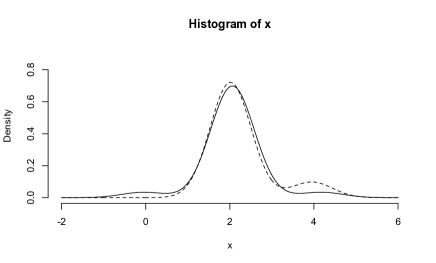
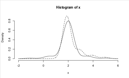
$NM_{3}$	$NM_{5}$

Figure 2: Histogram of tomato roots data with the estimated density under the unconstrained (dashed line) and constrained (solid line) NM₃ and NM₅ models.

5 Concluding remarks

After having reviewed the literature concerning the issue of testing for symmetry, in this contribution we outlined the existence of an interesting framework so far ignored, at least to our knowledge, to perform this test: that of normal mixture (NM) models. Indeed, NM models represent a semiparametric method to approximate unknown continuous densities with a satisfying goodness of fit, most of all in presence of skewness. Therefore, they offer a natural setting in which to place the study of symmetry of a distribution.

We first described the main characteristics of an NM model, illustrating in detail the EM algorithm implemented for parameter estimation. Then, we formulated the hypothesis test at issue in terms of constraints on weights characterising the NM model. Moreover, we describe how a likelihood ratio test is obtained, based on a test-statistic distributed according to a Chi-square with a number of degrees of freedom depending on the number of constraints and, therefore, on the number of mixture components.

A Monte Carlo study outlined how the performance of the proposed test depends on the criterion used to select the number of mixture components. More precisely, we observed that using BIC a good empirical level of significance is obtained, comparable with that of the traditional test based on the third standardised moment (Gupta,, 1967). On the other hand, the empirical power of our test with BIC resulted usually better than that observed with Gupta’s test.

An analysis on real data about the process of later root initiation in tomatoes illustrated the application of the proposed mixture-based test. Both criteria used to select the number of mixture components allowed to conclude about the skewness of distribution, as opposed to Gupta’s test, and to describe in detail the unknown underlying distribution from which data come.

References

- Abd-Elfattah and Butler, (2011) Abd-Elfattah, E. and Butler, R. (2011). Tests for symmetry with right censoring. Journal of Applied Statistics, 38(4):683–693.
- Akaike, (1973) Akaike, H. (1973). Information theory and an extension of the maximum likelihood principle. In Petrov, B. N. and Csaki, F., editors, Second International symposium of information theory, pages 267–281, Budapest. Akademiai Kiado.
- Bickel, (1982) Bickel, P. (1982). On adaptive estimation. Annals of Statistics, 10:647–671.
- Bonferroni, (1933) Bonferroni, C. (1933). Elementi di statistica generale. E. Gili.
- Cabilio and Masaro, (1996) Cabilio, P. and Masaro, J. (1996). As imple test of symmetry about an unknown median. The Canadian Journal of Statistics, 24:349–361.
- Cassart et al., (2011) Cassart, D., Hallin, M., and Paindaveine, D. (2011). A class of optimal tests for symmetry based on local edgeworth approximations. Bernoulli, 17(3):1063–1094.
- D’Agostino, (1970) D’Agostino, R. (1970). Transformation to normality of the null distribution of g1. Biometrika, 57(3):679–681.
- D’Agostino et al., (1990) D’Agostino, R., Belanger, A., and D’Agostino, R. (1990). A suggestion for using powerful and informative tests of normality. The American Statistician, 44(4):316–321.
- D’Agostino and Pearson, (1973) D’Agostino, R. and Pearson, E. (1973). Tests for departure from normality. empirical results for the distributions of b2 and b1. Biometrika, 60(3):613–622.
- Dempster et al., (1977) Dempster, A. P., Laird, N. M., and Rubin, D. B. (1977). Maximum likelihood from incomplete data via the EM algorithm (with discussion). Journal of the Royal Statistical Society, Series B, 39:1–38.
- Escobar and West, (1995) Escobar, M. and West, M. (1995). Bayesian density estimation and inferences using mixtures. Journal of the American Statistical Association, 90:577–588.
- Fan and Gencay, (1995) Fan, Y. and Gencay, R. (1995). A consistent nonparametric test of symmetry in linear regression models. Journal of American Statistical Association, 90(430):551–557.
- Ferguson, (1983) Ferguson, T. (1983). Bayesian density estimation by mixtures of normal distributions. In Rizvi, M., Rustagi, J., and Siegmund, D., editors, Recent advances in Statistics: papers in honor of Herman Chernoff on his Sixtieth Birthday, pages 287–302. Academic Press.
- Gupta, (1967) Gupta, M. (1967). An asymptotically non parametric test of symmetry. The Annals of Mathematical Statistics, 38(3):849–866.
- Gutierrez et al., (1995) Gutierrez, R., Carroll, R., Wang, N., Lee, G., and Taylor, B. (1995). Analysis of tomato root initiation using a normal mixture distribution. Biometrics, 51:1461–1468.
- Holgersson, (2010) Holgersson, T. (2010). A modified skewness measure for testing asymmetry. Communication in Statistics - Simulation and Computation, 39(2):335–346.
- Hollander, (1988) Hollander, M. (1988). Testing for symmetry, volume 9, pages 211–216. Wiley, New York.
- Hollander, (2006) Hollander, M. (2006). Testing for symmetry. Wiley, New York.
- Johnson and Kotz, (1970) Johnson, N. and Kotz, S. (1970). Continuous Univariate Distributions 1. Houghton Mifflin.
- Ley and Paindaveine, (2009) Ley, C. and Paindaveine, D. (2009). Le cam optimal tests for symmetry against ferreira and steel’s general skewed distributions. Journal of Nonparametric Statistics, 21(8):943–967.
- Lindsay, (1996) Lindsay, B. (1996). Mixture Models: Theory, Geometry and Applications. Institute of Mathematical Statistic.
- McLachlan and Peel, (2000) McLachlan, G. and Peel, D. (2000). Finite mixture models. Wiley.
- McWilliams, (1990) McWilliams, T. (1990). A distribution-free test for symmetry based on a runs statistic. Journal of the American Statistical Association, 85(412):1130–1133.
- Miao et al., (2006) Miao, W., Gel, Y., and Gastwirth, J. L. (2006). Random Walk, Sequential Analysis and Related Topics - A Festschrift in Honor of Yuan-Shih Chow, chapter A new test of symmetry about an unknown median. World Scientific.
- Mira, (1999) Mira, A. (1999). Distribution-free test of symmetry based on bonferroni’s measure. Journal of Applied Statistics, 26(8):959–971.
- Modarres and Gastwirth, (1996) Modarres, R. and Gastwirth, J. (1996). A modified runs test for symmetry. Statistics & Probability Letters, 31:107–112.
- Ngatchou-Wandii, (2006) Ngatchou-Wandii, J. (2006). On testing for the nullity of some skewness coefficients. International Statistical Review, 74(1):47–65.
- Ord, (1968) Ord, J. (1968). Annals of Mathematical Statistics, 39:1513–1516.
- Pearson, (1894) Pearson, K. (1894). Contributions to the theory of mathematical evolution. Philosophical Transactions of the Royal Society of London A, 185:71–110.
- Racine and Maasoumi, (2007) Racine, J. and Maasoumi, E. (2007). A versatile and robust metric entropy test of time-reversibility, and other hypotheses. Journal of Econometrics, 138:547–567.
- Randles et al., (1980) Randles, R., Fligner, M., Policello II, G., and Wolfe, D. (1980). An asymptotically distribution-free test for symmetry versus asymmetry. Journal of the American Statistical Association, 75(369):168–172.
- Robert, (1996) Robert, C. (1996). Mixtures of distributions: inference and estimation. In Gilks, W., Richardson, S., and Spiegelhalter, D., editors, Markov Chain Monte Carlo in Practice, pages 441–464. Chapman & Hall.
- Roeder and Wasserman, (1997) Roeder, K. and Wasserman, L. (1997). Practical density estimation using mixtures of normals. Journal of the American Statistical Association, 92:894 – 902.
- Schwarz, (1978) Schwarz, G. (1978). Estimating the dimension of a model. Annals of Statistics, 6(2):461–464.
- Titterington et al., (1985) Titterington, D. M., Smith, A. F. M., and Markov, U. E. (1985). Statistical analysis of Finite Mixture Distributions. John Wiley, New York.
- Yule, (1911) Yule, G. (1911). Introduction to the theory of statistics. Griffin.
- Zheng and Gastwirth, (2010) Zheng, T. and Gastwirth, J. L. (2010). On bootstrap tests of symmetry about an unknown median. Journal of Data Science, 8(3):413–427.