A Privacy-Aware Bayesian Approach for Combining Classifier and Cluster Ensembles
Abstract
This paper introduces a privacy-aware Bayesian approach that combines ensembles of classifiers and clusterers to perform semi-supervised and transductive learning. We consider scenarios where instances and their classification/clustering results are distributed across different data sites and have sharing restrictions. As a special case, the privacy aware computation of the model when instances of the target data are distributed across different data sites, is also discussed. Experimental results show that the proposed approach can provide good classification accuracies while adhering to the data/model sharing constraints.
I Introduction
Extracting useful knowledge from large, distributed data repositories can be a very difficult task when such data cannot be directly centralized or unified as a single file or database due to a variety of constraints. Recently, there has been an emphasis on how to obtain high quality information from distributed sources via statistical modeling while simultaneously adhering to restrictions on the nature of the data or models to be shared, due to data ownership or privacy issues. Much of this work has appeared under the moniker of “privacy-preserving data mining”.
Three of the most popular approaches to privacy-preserving data mining techniques are: (i) query restriction to solve the inference problem in databases [10] (ii) subjecting individual records or attributes to a “privacy preserving” randomization operation and subsequent recovery of the original data [3], (iii) using cryptographic techniques for secure two-party or multi-party communications [18]. Meanwhile, the notion of privacy has expanded substantially over the years. Approaches such as -anonymity and -diversity [14] focused on privacy in terms of indistinguishableness of one record from others under allowable queries. More recent approaches such as differential privacy [8] tie the notion of privacy to its impact on a statistical model.
The larger body of distributed data mining techniques developed so far have focused on simple classification/clustering algorithms or on mining association rules [2, 5, 9, 13]. Allowable data partitioning is also limited, typically to vertically partitioned or horizontally partitioned data [7]. These techniques typically do not specifically address privacy issues, other than through encryption [20]. This is also true of earlier, data-parallel methods [7] that are susceptible to privacy breaches, and also need a central planner that dictates what algorithm runs on each site. In this paper, we introduce a privacy-aware Bayesian approach that combines ensembles of classifiers and clusterers and is effective for both semi-supervised and transductive learning. As far as we know, this topic has not been addressed in the literature.
The combination of multiple classifiers to generate an ensemble has been proven to be more useful compared to the use of individual classifiers [17]. Analogously, several research efforts have shown that cluster ensembles can improve the quality of results as compared to a single clusterer — e.g., see [21] and references therein. Most of the motivations for combining ensembles of classifiers and clusterers are similar to those that hold for the standalone use of either classifier or cluster ensembles. However, some additional nice properties can emerge from such a combination. For instance, unsupervised models can provide supplementary constraints for classifying new data and thereby improve the generalization capability of the resulting classifier. Having this motivation in mind, a Bayesian approach to combine cluster and classifier ensembles in a privacy-aware setting is presented. We consider that a collection of instances and their clustering/classification algorithms reside in different data sites.
The idea of combining classification and clustering models has been introduced in the algorithms described in [11, 1]. However, these algorithms do not deal with privacy issues. Our probabilistic framework provides an alternative approach to combining class labels with cluster labels under conditions where sharing of individual records across data sites is not permitted. This soft probabilistic notion of privacy, based on a quantifiable information-theoretic formulation, has been discussed in detail in [15].
II BC3E Framework
II-A Overview
Consider that a classifier ensemble previously induced from training data is employed to generate a set of class labels for every instance in the target data. Also, a cluster ensemble is applied to the target data to provide sets of cluster labels. These class/cluster labels provide the inputs to Bayesian Combination of Classifier and Cluster Ensembles (BC3E) algorithm.
II-B Generative Model
Consider a target set formed by unlabeled instances. Suppose that a classifier ensemble composed of classification models has produced class labels (not necessarily different) for every instance . Similarly, consider that a cluster ensemble comprised of clustering algorithms has generated cluster labels for every instance in the target set. Note that the cluster labeled as 1 in a given data partition may not align with the cluster numbered 1 in another partition, and none of these clusters may correspond to class 1. Given the class and cluster labels, the objective is to come up with refined class probability distributions of the target set instances. To that end, assume that there are classes, which are denoted by . The observed class and cluster labels are denoted by where is the class label of the instance for the classifier and is the cluster label assigned to the instance by the clusterer. A generative model is proposed to explain the observations , where each instance has an underlying mixed-membership to the different classes. Let denote the latent mixed-membership vector for . It is assumed that – a discrete probability distribution over the classes – is sampled from a Dirichlet distribution, with parameter . Also, for the classes (indexed by ) and different base clusterings (indexed by ), we assume a multinomial distribution over the cluster labels. If the base clustering has clusters, is of dimension and . The generative model can be summarized as follows. For each :
-
1.
Choose .
-
2.
, choose .
-
3.
.
-
(a)
Choose where is a vector of dimension with only one component being unity and others being zero.
-
(b)
Choose .
-
(a)
If the instance is sampled from the class in the base clustering (implying ), then its cluster label will be sampled from the multinomial distribution . Modeling of the classification results from different classifiers for the instance is straightforward: the observed class labels () are assumed to be sampled from the latent mixed-membership vector . In essence, the posteriors of are expected to get more accurate in an effort to explain both classification and clustering results (i.e. ) in the same framework. BC3E derives its inspiration from the mixed-membership naïve Bayes model [19].
To address the log-likelihood function of BC3E, let us denote the set of hidden variables by . The model parameters can conveniently be represented by . Therefore, the joint distribution of the hidden and observed variables can be written as:
| (1) | |||||
In theory, inference and estimation with the proposed model could be performed by maximizing the log-likelihood in Eq. (1) – using the Expectation Maximization family of algorithms [6]. However, the coupling between and makes the exact computation in the summation over the classes intractable in general [4]. Therefore, inference and estimation is performed using Variational Expectation Maximization (VEM) [12].
II-C Approximate Inference and Estimation
II-C1 Inference
To obtain a tractable lower bound on the observed log-likelihood, we specify a fully factorized distribution to approximate the true posterior of the hidden variables:
| (2) |
where , and , and , which is the set of variational parameters corresponding to the instance. Further, , , and ; where the components of the corresponding vectors are made explicit. Using Jensen’s inequality, a lower bound on the observed log-likelihood can be derived:
| (3) | |||||
where is the entropy of the variational distribution , and is the expectation w.r.t . It turns out that the inequality in (3) is due to the non-negative KL divergence between and – the true posterior of the hidden variables. Let be the set of all distributions having a fully factorized form as given in (2). The optimal distribution that produces the tightest possible lower bound is thus given by:
| (4) |
The optimal value of that satisfies (4) is given by
| (5) |
where, if the cluster label of the instance in the clustering is and otherwise. Since is a multinomial distribution, the updated values of the components should be normalized to unity. Similarly, the optimal value of that satisfies (4) is given by:
| (6) |
Note that the optimal values of depend on and vice-versa. Therefore, iterative optimization is adopted to minimize the lower bound till convergence is achieved.
II-C2 Estimation
For estimation, we maximize the optimized lower bound obtained from the variational inference w.r.t the free model parameters (by keeping the variational parameters fixed). Taking the partial derivative of the lower bound w.r.t we have:
| (7) |
Again, since is a multinomial distribution, the updated values of components should be normalized to unity. However, no direct analytic form of update exists for (see [4] for more details) and a numerical method for optimization needs to be resorted to111We use a Newton-Raphson based update procedure as suggested in [16]. The part of the objective function that depends on is given by:
| (8) | |||||
Note that the optimization has to be performed with the constraint . Once the optimization in M-step is done, E-step starts and the iterative update is continued till convergence.
III Privacy Aware Computation
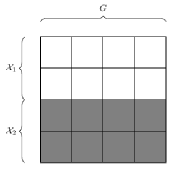
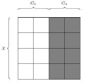
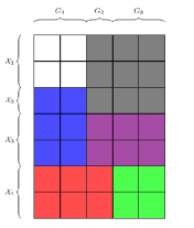
Inference and estimation using VEM allows performing computation without explicitly revealing the class/cluster labels. One can visualize instances, along with their class/cluster labels, arranged in a matrix form so that each data site contains a subset of the matrix entries. Depending on how the matrix entries are distributed across different sites, three scenarios can arise – i) Row Distributed Ensemble, ii) Column Distributed Ensemble, and iii) Arbitrarily Distributed Ensemble.


![[Uncaptioned image]](/html/1204.4521/assets/x4.png)
III-A Row Distributed Ensemble
In the row distributed ensemble framework, the target set is partitioned into different subsets, which are assumed to be at different locations. The instances from subset are denoted by , so that . It is assumed that class and cluster labels are available – i.e., they have already been generated by some classification and clustering algorithms. The objective is to refine the class probability distributions (obtained from the classifiers) of the instances from without sharing the class/cluster labels across the data sites.
A careful look at the E-step – Equations (5) and (6) – reveals that the update of the variational parameters corresponding to each instance in a given iteration is independent of those of other instances given the model parameters from the previous iteration. This suggests that we can maintain a client-server based framework, where the server only updates the model parameters (in the M-step) and the clients (corresponding to individual data sites) update the variational parameters of the instances in the E-step. For instance, consider a situation (shown in Fig. 3) where a target dataset is partitioned into two subsets, and , and that these subsets are located in two different data sites. The data site has access to and accordingly, to the respective class and cluster labels of their instances. Similarly, the data site has access to the instances of and their class/cluster labels.
Now, data site can update the variational parameters . Similarly, data site can update the variational parameters . Once the variational parameters are updated in the E-step, the server gathers information from the two sites and updates the model parameters. Here, the primary requirement is that the class and cluster labels of instances from different data sites should not be available to the server. Now, Eq. (7) can be broken as follows:
| (9) |
The first and second terms can be calculated in data sites and , separately, and then sent to the server, where the two terms can be added and can get updated . The variational parameters are not available to the sever and thus only some aggregated information about the values of for some is sent to the server. We also observe that more the number of instances in a given data site, more difficult it becomes to retrieve the cluster labels (i.e. ) from individual clients. Also, in practice, the server does not get to know how many instances are present per data site which only makes the recovery of cluster labels even more difficult. Also note that the approach adopted only splits a central computation in multiple tasks based on how the data is distributed. Therefore, the performance of the proposed model with all data in a single place should always be the same as the performance with distributed data assuming there is no information loss in data transmission from one node to another.
In summary, the server, after updating in the M-step, sends them out to the individual clients. The clients, after updating the variational parameters in the E-step, send some partial summation results in the form shown in Eq. (9) to the server. The server node is helpful for the conceptual understanding of the parameter update and sharing procedures. In practice, however, there is no real need for a server. Any of the client nodes can itself take the place of server, provided that the computations are carried out in separate time windows and in proper order.
III-B Column and Arbitrarily Distributed Ensemble
The column and arbitrarily distributed ensembles are illustrated in Figs. 3 and 3 respectively. Analogous distributed inference and estimation frameworks can be derived in these two cases without sharing the cluster/class labels among different data sites. However, detailed discussion is avoided due to space constraints.
IV Experimental Evaluation
We have already shown, theoretically, that the classification results obtained by the privacy-aware BC3E are precisely the same as those we would have gotten if all the information originally distributed across different data sites were available at a single data site. Therefore, we assess the learning capabilities of BC3E using five benchmark datasets (Heart, German Numer, Halfmoon, Wine, and Pima Indians Diabetes) — all stored in a single location. Semi-supervised approaches are most useful when labeled data is limited, while these benchmarks were created for evaluating supervised methods. Therefore, we use only small portions (from 2% to 10%) of the training data to build classifier ensembles. The remaining data is used as a target set — with the labels removed. We adopt 3 classifiers (Decision Tree, Generalized Logistic Regression, and Linear Discriminant). For clustering, we use hierarchical single-link and -means algorithms. The achieved results are presented in Table I, where Best Component indicates the accuracy of the best classifier of the ensemble. We also compare BC3E with two related algorithms (C3E [1] and BGCM [11]) that do not deal with privacy issues. One can observe that, besides having the privacy-preserving property, BC3E presents competitive accuracies with respect to their counterparts. Indeed, the Friedman test, followed by the Nemenyi post-hoc test for pairwise comparisons between algorithms, shows that there is no significant statistical difference () among the accuracies of BC3E, C3E, and BGCM.
V Extension and Future Work
The results achieved so far motivate us to employ soft classification and clustering. Applications of BC3E to real-world transfer learning problems are also in order.
Acknowledgments
This work was supported by NSF (IIS-0713142 and IIS-1016614) and by the Brazilian Agencies FAPESP and CNPq.
References
- [1] A. Acharya, E. R. Hruschka, J. Ghosh, and S. Acharyya. C3E: A Framework for Combining Ensembles of Classifiers and Clusterers. In 10th Int. Workshop on MCS, 2011.
- [2] D. Agrawal and C. C. Aggarwal. On the design and quantification of privacy preserving data mining algorithms. In Symposium on Principles of Database Systems, 2001.
- [3] R. Agrawal and R. Srikant. Privacy-preserving data mining. In ACM SIGMOD, pages 439–450, 2000.
- [4] D. M. Blei, A. Y. Ng, and M. I. Jordan. Latent dirichlet allocation. JMLR, 3:993–1022, 2003.
- [5] P. Chan, S. Stolfo, and D. Wolpert (Organizers). Integrating multiple learned models. Workshop with AAAI’96, 1996.
- [6] A. P. Dempster, N. M. Laird, and D. B. Rubin. Maximum likelihood from incomplete data via the EM algorithm. J. Royal Statistical Society. Series B (Methodological), 39(1):1–38, 1977.
- [7] I. S. Dhillon and D. S. Modha. A data-clustering algorithm on distributed memory multiprocessors. In Proc. Large-scale Parallel KDD Systems Workshop, ACM SIGKDD, August 1999.
- [8] C. Dwork and J. Lei. Differential privacy and robust statistics. In STOC, pages 371–380, 2009.
- [9] A. Evfimievski, R. Srikant, R. Agrawal, and J. Gehrke. Privacy preserving mining of association rules. In KDD, 2002.
- [10] C. Farkas and S. Jajodia. The inference problem: A survey. SIGKDD Explorations, 4(2):6–11, 2002.
- [11] J. Gao, F. Liang, W. Fan, Y. Sun, and J. Han. Graph-based consensus maximization among multiple supervised and unsupervised models. In Proc. of NIPS, pages 1–9, 2009.
- [12] M. I. Jordan, Z. Ghahramani, T. S. Jaakkola, and L. K. Saul. An introduction to variational methods for graphical models. Mach. Learn., 37(2):183–233, 1999.
- [13] Y. Lindell and B. Pinkas. Privacy preserving data mining. LNCS, 1880:36–77, 2000.
- [14] A. Machanavajjhala, D. Kifer, J. Gehrke, and M. Venkitasubramaniam. ℓ-diversity: Privacy beyond k-anonymity. In ICDE, 2006.
- [15] S. Merugu and J. Ghosh. Privacy perserving distributed clustering using generative models. In Proc. of ICDM, pages 211–218, Nov, 2003.
- [16] T. P. Minka. Estimating a dirichlet distribution. Technical report, 2003.
- [17] N. C. Oza and K. Tumer. Classifier ensembles: Select real-world applications. Inf. Fusion, 9:4–20, January 2008.
- [18] B. Pinkas. Cryptographic techniques for privacy-preserving data mining. SIGKDD Explorations, 4(2):12–19, 2002.
- [19] H. Shan and A. Banerjee. Mixed-membership naive bayes models. Data Min. Knowl. Discov., 23:1–62, July 2011.
- [20] J. Vaidya and C. Clifton. Privacy-perserving k-means clustering over vertically patitioned data. In KDD, pages 206–215, 2003.
- [21] H. Wang, H. Shan, and A. Banerjee. Bayesian cluster ensembles. Statistical Analysis and Data Mining, 1:1–17, January 2011.