A CLASSIFICATION OF H II REGIONS BASED ON OXYGEN AND HELIUM LINES: THE CASES OF TOL 2146$-$391 AND TOL 0357$-$3915

Abstract

We present long slit spectrophotometry of two H II galaxies: TOL 2146$-$391 and TOL 0357$-$3915. We performed a detailed analysis that involves abundance determinations relaxing the assumption of homogeneous temperature. The temperature inhomogeneities values, $t^{2}$, were obtained through two methods: (i) comparing abundances from oxygen recombination lines to abundances from collisionally excited lines and (ii) by using the line intensity ratios of a set of He I lines together with the helio10 program. We find that the helio10 program is a good alternative to obtain a $t^{2}$ value in photoionized regions where recombination lines of heavy elements are not available. We have plotted 27 high and low metallicity H II regions in an oxygen degree of ionization versus $t^{2}$ diagram; we find areas populated by H II regions and areas void of them; the physical characteristics of each area are discussed. In addition, an average $t^{2}$ value can be determined for the objects in each area. We propose to use this $\langle t^{2}\rangle$ value for the cases where a direct measurement of $t^{2}$ cannot be determined.

1 Introduction

H II region chemical abundances provide observational constrains that allow to test models of Galactic chemical evolution through, for example, the determination of radial abundance gradients in spiral galaxies (Vila-Costas & Edmunds, 1992; Zaritsky et al., 1994). In addition to this, results derived from nebular studies are used in the field of starburst galaxies which, along with other physical properties such as luminosity or the mass-metallicity relation, allow us to study the chemical enrichment of the Universe (e.g. Tremonti et al., 2004; Pérez-Montero et al., 2008; Liu et al., 2008; Peimbert & Peimbert, 2011). It is therefore of great importance for these studies to use accurate abundance determinations.

However, there exists an important problem of inconsistency between the abundances determined with recombination lines (RLs) and those determined with collisionally excited lines (CELs) assuming homogeneous temperature. This is usually refered to as the abundance discrepancy factor (ADF) problem. Arguments in favor of determining abundances from CELs with homogeneous temperature are given by Bresolin et al. (2009); Ercolano et al. (2010); Rodríguez & García-Rojas (2010), among others. Arguments in favor of determining abundances from RLs are given bellow.

There are two main sets of explanations that have been proposed in the literature to reconcile the abundances from CELs and from RLs, thus solving the ADF problem: (i) temperature inhomogeneities within a chemically homogeneous medium, these inhomogeneities would come from shock waves, shadowed regions, advancing ionization fronts, multiple ionizing sources, X-rays, and magnetic reconnection, among others (e.g. Peimbert & Peimbert, 2006, and references therein); and (ii) high metallicity inclusion, which also imply temperature inhomogeneities, these inclusions would be surviving gas from supernova remnants that has not fully mixed with the interstellar medium (e.g. Tsamis & Péquignot, 2005; Stasińska et al., 2007, and references therein). Both sets of explanations indicate underabundant results when using CELs and homogeneous temperature to determine abundances. One example of temperature inhomogeneities within a chemically homogeneous medium is given in Peimbert (2003), where a careful study of 30 Doradus was done assuming a chemically homogeneous medium and the obtained abundances were 0.21 dex higher than those obtained using CELs and homogeneous temperature. An example of high metallicity inclusions is given by Tsamis & Péquignot (2005), whom created a model for 30 Doradus including chemical inhomogeneities that resulted in abundances 0.09 dex lower than those obtained from RLs and 0.12 dex higher than abundances obtained from CELs and homogeneous temperature.

In favor of the abundances derived from RLs is the consistency found in many studies of the chemical evolution of our own Galaxy. Abundances derived from H II regions considering the O depletion into dust grains and thermal inhomogeneities (Carigi & Peimbert, 2011; Peimbert & Peimbert, 2011) are consistent with: (i) the protosolar abundances corrected by 4.5 Gyr of chemical evolution (Asplund et al., 2009; Carigi & Peimbert, 2011), (ii) the abundances of young F and G stars of the solar vicinity (Bensby & Feltzing, 2006), and (iii) the abundances of O and B stars of the Orion region (Przybilla et al., 2008; Simón-Díaz & Stasińska, 2011). Throughout this paper we will assume a chemically homogeneous medium and that the abundances are given by RLs or by CELs and considering the presence of thermal inhomogeneitites.

Peimbert (1967) first recognized the possibility of including thermal inhomogeneities in studies of photoionized regions; later on, Peimbert & Costero (1969) studied the magnitude of the effect of such thermal inhomogeneities on the determination of chemical abundances. These two articles introduced the formalism of temperature inhomogeneities ($t^{2}$) to determine chemical abundances; in them, it is found that H II region abundances obtained through the traditional method —which involves assuming a homogeneous temperature throughout the whole volume of the object, usually obtained from the [O III] line ratio $\lambda\lambda$ 4363/(4959+5007)— were underestimated by a factor of approximately 2.5 (although, the exact $t^{2}$ value is object dependent and its effect on the abundances is also temperature dependent).

With the availability of large telescopes, it has been possible to use the formalism of $t^{2}$ to study the ADF. Several studies have shown that ADF typical values are in the 1.5 - 3 range for most H II regions (e.g. Peimbert et al., 1993, 2005; García-Rojas & Esteban, 2007; Peimbert et al., 2007; Esteban et al., 2009), and in the 1.5 - 5 range for most Planetary Nebulae (e.g. Liu & Danziger, 1993; Peimbert et al., 1995; Stasińska & Szczerba, 2001; Liu, 2006; Peimbert & Peimbert, 2006). Since CELs lead to underestimate abundances when ignoring the presence of temperature inhomogeneities, we consider that abundances determined from RLs are more reliable.

For chemically homogeneous objects, it is possible to derive accurate abundances from RL ratios (that are independent of $t^{2}$), as well as from CELs adopting a $t^{2}$ value. There are several ways to determine $t^{2}$ values (see Peimbert, 1967; Peimbert & Peimbert, 2011). The two most frequently used are: (i) from the comparison of abundances derived from [O III] lines with those derived from O II lines (this basically indicates what value of $t^{2}$ is required for CELs to reproduce the RL abundances) and (ii) from the comparison of the temperature of forbidden lines to that of the Balmer continuum (this can give accurate O/H abundances without measuring oxygen RLs). Heavy element RLs are particularly faint in low metallicity H II regions such as the ones presented in this paper; moreover, the Balmer discontinuity is smaller and less sensitive at higher temperatures. There is a third method based on He I lines which has been previously used and which will be further discussed in this paper. For low metallicity objects, where the oxygen RLs are too faint to be measurable and the Balmer discontinuity is very difficult to measure, He I lines can play a key role in abundance determinations.

Unfortunately, there are some H II regions where a precise value of $t^{2}$ cannot be acquired, for instance H II galaxies with high redshift or low intrinsic brightness. In this scenarios it is important to recognize that, statistically speaking, a good assumption of the value of $\langle t^{2}\rangle$ is much better than assuming that $t^{2}$=0.00. For those objects, it should be possible to use an average $t^{2}$ value obtained from most of the $t^{2}$ determinations of H II regions in the literature. In this paper we derive a value of this average for high and low metallicity H II regions, $\langle t^{2}\rangle$.

In Sections 2 and 3 we present the observations of TOL 2146$-$391 and TOL 0357$-$3915 as well as a description of the reduction procedure. The characteristics of the code helio10 are presented in Section 4. In Section 5 we derive temperatures and densities, as well as the available $t^{2}$ values. The ionic abundance determinations based on the ratios of CELs to RLs, and based on RLs alone are presented in Section 6. In Section 7 we determine the total abundances. In Section 8 we present a review of the $t^{2}$ values in the literature and recommend an average $t^{2}$ value for those objects where a particular $t^{2}$ is not available. Finally, in Section 9 we present the summary and conclusions.

2 Observations

The two galaxies presented in this paper were observed in order to increase the number of low metallicity objects with high S/N. Objects of this kind are very useful to study the chemical evolution of galaxies with low SFR, to determine the primordial helium abundance, and to calibrate the lower branch of Pagel’s method to determine oxygen abundaces.

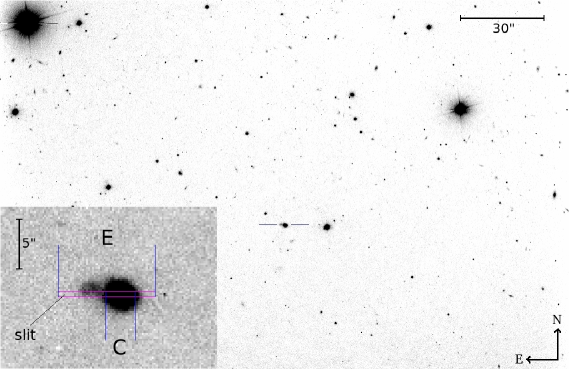
(a)


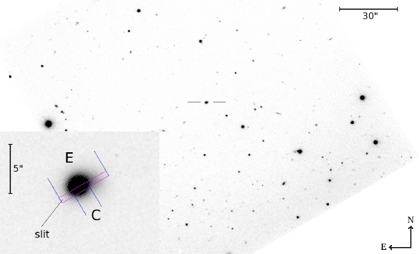
(b)

Figure 1: (1a) VLT images of TOL 2146$-$391 and (1b) of TOL 0357$-$3915. These objects are located at $\alpha=21^{h}49^{m}48.2^{s}$ and $\delta=-38^{\circ}54^{\prime}08.6^{\prime\prime}$ and $\alpha=03^{h}59^{m}08.9^{s}$, $\delta=-39^{\circ}06^{\prime}23.0"$ (J2000.0), respectively. Their redshifts are $z$=0.0295 for TOL 2146$-$391 and $z$=0.0744 for TOL 0357$-$3915.

The long slit spectrophotometry presented in this work was obtained at the VLT Melipal facility in Chile, with the Focal Reducer Low Dispersion Spectrograph 1, FORS1. Three grism settings where used: GRIS-600B+12, GRIS-600R+14 with filter GG435, and GRIS-300V with filter GG375 (see Table 1). Observations were made on September 10^th and 11^th of 2002 for TOL 2146$-$391 ($\alpha=21^{h}49^{m}48.2^{s}$, $\delta=-38^{\circ}54^{\prime}08.6"$) and TOL 0357$-$3915 ($\alpha=03^{h}59^{m}08.9^{s}$, $\delta=-39^{\circ}06^{\prime}23.0"$), respectively (see Figure 1).

The slit was 0.51” wide and 410” long for both H II galaxies, TOL 2146$-$391 and TOL 0357$-$3915. The slit was oriented with a position angle of 90^∘ to observe TOL 2146$-$391, and 60^∘ for TOL 0357$-$3915. The linear atmospheric dispersion corrector, was used to keep the same observed region within the slit regardless of the air mass value. The wavelength coverage and the resolutions for the emission lines observed with each grism are given in Table 1. The average seeing during the observations amounted to 0.74” for TOL 2146$-$391 and 0.88” for TOL 0357$-$3915.

We took two extractions from each object, Extraction C stands for the core of each H II region, while Extraction E stands for each extended H II region. In TOL 2146$-$391 Extractions C and E had 15 pixels (3.0”) and 49 pixels (9.8”), respectively; while for TOL 0357$-$3915 Extractions C and E had 9 (1.8”) and 27 pixels (5.4”), respectively. Extractions C are centered at the brightest region while Extractions E are slightly displaced in order to include most of the emission (see Figure 1). For TOL 2146$-$391, Extraction C included 94% of the flux included in Extraction E, and for TOL 0357$-$3915, Extraction C included 88% of the total flux of Extraction E. We decided to present the analysis of both extractions of both objects for several reasons: (i) we were trying to obtain as much information as possible with the highest precision available, (ii) we were looking to see if there were drastic differences between the central and the outer parts of each extraction (notice the plots present in the inserts), (iii) we were looking for the determination with the best S/N available, and (iv) both analysis were completely independed and helped us to better estimate the errors in the line intensity determinations.

The spectra were reduced using IRAF, following the standard procedure of bias subtraction, aperture extraction, flatfielding, wavelength calibration, and flux calibration. For flux calibration the standard stars LTT 2415, LTT 7389, LTT 7987, and EG 21 were used (Hamuy et al., 1992, 1994). The observed spectra are presented in Figure 2.

3 Line Intensities and Reddening Correction

The splot task of the IRAF package was used for line measurements. Line intensities were obtained by integrating the flux in the line between two limits over the local continuum estimated by eye. When line blending was present, a multiple Gaussian profile was used to determine the line intensities.

We used the measurements of the Balmer decrement of the low resolution spectra to tie the blue and red high resolution spectra. The emission line intensities of all extractions in TOL 2146$-$391 and in TOL 0357$-$3915 are presented in Tables 2 and 3, respectively.

To determine the reddening correction we compared the theoretical Balmer line intensity ratios with the observed ones. A proper determination of the reddening correction is always desired, in this work it is required to allow helio10 to be able to extract all the possible information from the He I lines that span from $\lambda\lambda$ 3634 to 7281.

The observed Balmer line intensities have to be corrected for reddening, underlying absorption, and collisional excitation before they can be compared to the theoretical recombination intensities; also both —the theoretical Balmer recombination intensities and the collisional Balmer excitation intensities— depend on the temperature; and to obtain estimates of the temperature it is necessary to use dereddened line intensity ratios. This means that all four quantities need to be fitted self-consistently.

A first approximation to the correction for the reddening coefficients, $C$(H$\beta$)s, is obtained by ignoring underlying absorption and collisional excitation, adopting $T_{e}=$10,000 K, and fitting the observed and theoretical $I$(H$\alpha$)/$I$(H$\beta$) ratios. This reddening correction is applied to the [O III] lines to obtain $T_{e}$[O III]. This approximation will be enough to determine (i) the theoretical intensities of the Balmer lines —that are only weakly dependent on the temperature—, and (ii) the contribution of collisional excitation to the Balmer line intensities —that is small (Peimbert et al., 2007). Finally, the reddening correction and underlying absorption were fitted simultaneously taking advantage of the fact that reddening is more important for H$\alpha$, H$\beta$, and H$\gamma$, while underlying absorption is more important for the weaker bluer Balmer lines. (Notice that the contribution of He II $\lambda$ 4859 to H$\beta$ is less than one part in a thousand).

For both extractions of TOL 0357$-$3915, the best fit to the four brightest Balmer lines yielded an H$\beta$ greater than 100 (102.20 for Extraction C, and 100.80 for Extraction E), which is within the observational errors presented in Table 3. We took the unconventional decision of choosing this H$\beta$ value to give the proper weight to these four Balmer lines.

The theoretical Balmer recombination intensity ratios were obtained using the program INTRAT  (Storey & Hummer, 1995) assuming $T_{e}$=13,415 K and $n_{e}$=140 cm^-3 for TOL 2146$-$391, and $T_{e}$=12,570 K and $n_{e}$=120 cm^-3 for TOL 0357$-$3915 (forbidden line intensity ratios used to determine densities are not dependent on any of the parameters we are adjusting in this section). INTRAT stands for INTensity RATios of hydrogenic recombination lines for specified transitions.

The fraction of the Balmer line intensities due to collisional excitation from the ground state were estimated from interpolations to the models presented by Peimbert et al. (2007). This correction is not commonly used because it is very small for objects cooler than 12,000 K as well as for ionized regions that are density bounded. However, it is relevant to both, the proper determination of $C$(H$\beta$) and $I_{rec}$(H$\beta$), for these two objects; contributing with 3.8% and 3.2% for the $I$(H$\alpha$) of TOL 2146$-$391 and TOL 0357$-$3915, respectively. We normalized to $I_{rec}$(H$\beta$) because most of the formulas that compare line intensities to that of H$\beta$, implicitely assume that $I$(H$\beta$) represents the recombination cascade of the nebular component. Due to the energy level distribution, collisional excitation from the ground level is negligible for the observed permitted lines of all the other ions.

The reddening coefficients, were determined by assuming the extinction law of Seaton (1979), $f(\lambda)$. The values found for $C$(H$\beta$) as well as for the assumed $f(\lambda)$ are presented in Tables 2 and 3 for TOL 2146$-$391 and TOL 0357$-$3915, respectively.

The correction due to the underlying absorption equivalent widths for the Balmer lines was done using a stellar spectra template normalized to $EW_{abs}$(H$\beta$). The template is presented in Table 4 and the normalizations used are presented in Tables 2 and 3. The template was generated based on the low metallicity instantaneous burst models from González-Delgado et al. (1999). These absorption line ratios do not change considerably during the first 5 Myr, the numbers presented in Table 4 represent an average of the ratios of the models between 0 and 5 Myr. To complete the template we require H$\alpha$ and H7, M. Cerviño kindly ran for us some models with the same code as R. Gonźalez-Delgado and collaborators, and provided us with the $EW_{abs}$ for many lines required in this template. The high-n Balmer lines are too close to be separated in the spectra provided by this code; alternatively, it is possible to estimate the $EW_{abs}$ from a deep echelle observation of a young H II region. For these, we used the data of 30 Doradus obtained by Peimbert (2003), where we estimated the $EW_{abs}$(H high-n)/$EW_{abs}$(H$\beta$) required to adjust the observed Balmer lines to the theoretical ones. The $EW_{abs}$(H$\beta$) values we adopted do not correspond to any particular age, but do correspond to the intensities that best fit the high n Balmer lines to H$\beta$ ratios. Forbidden lines do not have underlying absorption, however, permitted lines do; underlying absorption equivalent widths used for the He I lines included in the template come from González-Delgado and colaborators as well as the additional models ran by Cerviño and are also presented in Table 4. The corrections to the line intensities due to underlying absorption of C II, N II, and O II are expected to be negligible, more than an order of magnitude smaller than our observational uncertainties, and were not considered.

Column (1) in Tables 2 and 3 presents the adopted laboratory wavelength, $\lambda$, and column (2) the identification for each line. Column (3) in both tables presents the extinction law value used for each line (Seaton, 1979). In both tables, columns (4-6) represent the data of the core extractions, Extraction C, while columns (7-9) represent the data of the extended extractions, Extraction E. Columns (4) and (7) include the observed flux relative to $F$(H$\beta$)=100.00, $F(\lambda)$; columns (5) and (8) include the flux corrected for reddening (as well as underlying absorption —for H I and He I lines— and collisional excitation —for H I lines) relative to $I_{rec}$(H$\beta$)=100.00, $I$($\lambda$); finally columns (6) and (9) include the error percentage associated with those intensities, which already include all the errors in $C$(H$\beta$), $EW_{abs}$(H$\beta$), and collisional excitation of the Balmer lines.

4 helio10

Recombination lines are not usually used to determine physical quantities of the ionized regions: the intensities of all H I lines are approximately proportional to $n_{e}n$(H${}^{+})T_{e}^{-0.9}$ so their ratios are nearly independent of $n_{e}$ and $T_{e}$; this is the reason they are ideal to determine the reddening correction. To determine $T_{e}$ using the Balmer discontinuity it is necessary to have an exquisitely accurate tailored made model of the stellar spectra, since about $80\%$ of the observed continuum is stellar and the Balmer discontinuity shows up in absorption (at very high densities it is possible to use high order Balmer lines to estimate $n_{e}$, e.g. Liu et al., 2000; Peimbert et al., 2004). He II lines are not more useful than H I lines to determine $n_{e}$ or $T_{e}$, plus, they are generally fainter. On the other hand, RLs of heavy elements could theoretically provide information to derive the physical conditions, but are usually too faint to do much with them (although very deep echelle observations of the O II multiplet 1 lines have been shown to be useful for $n_{e}$ determinations, e.g. Ruiz et al., 2003; Peimbert et al., 2005).

He I lines are a few orders of magnitude stronger than heavy element recombination lines and have a less homogeneous (more complicated) temperature and density dependence than RLs from hydrogenoid ions making He I lines the best RLs to determine physical conditions. The intensity of each He I line is proportional to $n_{e}n($H${}^{+})T_{e}^{-\alpha}$, however, each line has a slightly different $\alpha$ —for the brightest He I lines, $\alpha$ is in the 0.7 to 1.1 range— making it possible to determine the temperature from a ratio of He I lines. Also, adding information and complexity to the determinations, the metastable level 2³S produces an additional dependence on density and optical depth, $\tau$(2³S). The 2³S level is stable for 2.5 hours before radiatively decaying, thus providing enough excited atoms to produce an appreciable effect on (i) the optical depth to the n³P-2³S He I lines; these, in turn, affect many of the triplet lines (He I $\lambda\lambda$ 3889 and 7065 are the most affected optical lines); as well as (ii) an appreciable target for collisional excitations which in turn enhances all the optical He I lines (again, the most affected are He I $\lambda\lambda$ 3889 and 7065). In the end, each triplet He I line has a unique dependence on $n_{e}$, $T_{e}$, and $\tau$(2³S); while singlet He I lines depend on $n_{e}$ and $T_{e}$ (singlet lines are not affected by the opacity produced by the metastability of the 2³S level, they only depend weakly on the opacity produced by the —much smaller— metastability of the 2¹S level). Even with the additional complications of having one more variable, triplets tend to be better than singlets because they have approximately 3 times more intensity and have a stronger dependence on $n_{e}$.

Properly measured He I line intensities of the photoionized material (i.e. lines that have been properly corrected for the reddening produced by dust grains and for the underlying absorption present in the stellar spectra), can be used to determine the average physical conditions of such gas parcel. Theoretically, one needs at least four He I lines —three independent He I line ratios— to be able to solve for all the unknowns (i.e. $n_{e}$, $T_{e}$, and $\tau$(2³S) along with the $n$(He⁺)/$n$(H⁺) ratio); in practice, more lines are better since dependences on $n_{e}$, $T_{e}$, and $\tau$(2³S) is weak for most line ratios.

helio10 is an extension of the maximum likelihood method used in previous works to determine $t^{2}$(He⁺) (see , Peimbert et al.2000; Peimbert et al., 2002; Peimbert, 2003; Esteban et al., 2004; Peimbert et al., 2005). This version of the code can determine $T_{e}$(He I) using only He I line intensities. The code also yields $T_{0}$ and $t^{2}$ (the formal definitions are presented in Section 5.3) by combining the information of the He I lines with the information of the [O II] (7325/3727) and [O III] (4363/5007) line ratios.

The effective recombination coefficients for the H I and He I lines were those given by Storey & Hummer (1995) for H, and by Benjamin et al. (1999) and Porter et al. (2007) for He. The collisional contribution was estimated from Sawey & Berrington (1993) and Kingdon & Ferland (1995). The optical depth effects in the triplets were estimated from calculations made by (Benjamin et al.2002). The collisional strengths come from McLaughlin & Bell (1993) for [O II] and Lennon & Burke (1994) for [O III], while the transition probabilities come from Wiese et al. (1996).

In its simplest mode helio10 uses up to 20 He I/H$\beta$ ratios with their uncertainties to search for the most likely values for $T_{e}$(He I), $n_{e}$(He I), $\tau$(2³S), and $n$(He⁺)/$n$(H⁺). It firsts assumes a certain set of values and, using the relevant atomic data, estimates the theoretical He I/H$\beta$ ratios. Then, it compares the observed ratios to the theoretical ones determining

$$\chi^{2}=\sum\limits_{\lambda}{\left\{\left[{I({\lambda})\over I({\rm H\beta})}\right]_{obs}-\left[{I({\lambda})\over I({\rm H\beta})}\right]_{theo}\right\}^{2}\over\sigma_{I(\lambda)}^{2}}.$$ (1)

Using multidimensional optimization algorithms, helio10 then searches the parameter space looking for the minimum $\chi^{2}$ value, $\chi^{2}_{min}$; and, finally, it determines the available parameter space within $\chi^{2}_{min}\leq\chi^{2}\leq\chi^{2}_{min}+1$ to estimate the 1$\sigma$ error bars of each one of the four variables.

Additional constraints can be included to better determine the physical conditions of the nebula on any or all of the variables; any available determination independent of the He I lines can be used as an input (with the corresponding uncertainty). When the solution given by the He I lines alone is very uncertain, an additional constraint directly restricts one variable and indirectly restricts all the others; when the solution given by the He I lines alone has uncertainties of a similar magnitude as those given by the additional constraint, the output for that variable becomes a weighted average while the others become slightly better restricted (when using these additional constraints the corresponding variables will have an output that does not necessarily match the partial input).

In general the temperatures derived fom the He I line data are smaller than those derived from forbidden line data. When combining He I data with forbidden line data, to determine self-consistent physical conditions, instead of searching for $T_{e}$(He I) helio10 searches for $T_{0}$ and $t^{2}$ (as well as for $n_{e}$(He I), $\tau$(2³S), and $n$(He⁺)/$n$(H⁺)); this $T_{0}$ and $t^{2}$ together with a specific shape define a distribution of temperatures. helio10 simulates five types of temperature distributions: gaussian, square, symmetric triangle, left triangle, and right triangle. For a certain set of He I lines, the exact determination of $t^{2}$ depends on the shape of the distribution: right triangles require slightly larger $t^{2}$ than left triangles, and square distributions require slightly larger $t^{2}$ values than symmetric triangle distributions, gaussian distributions lie in the middle. The dispersion between the distributions is less than 10% on the $t^{2}$ values except for the most extreme cases. To be able to distinguish between these distributions using He I lines alone, the uncertainties in the intensity determinations would be required to be at least two orders of magnitude smaller than the observed ones; the recommended shape of the distribution depends on the mechanism responsible for the thermal inhomogeneities. For this work we will present the results obtained using gaussian distributions. helio10 does not model density variations, but the models are robust for H II regions because their densities usually are lower than the critical density of the 2³S level, $n_{crit}\approx 3,000\,{\rm cm}^{-3}$ (critical densities for the [O II] (7325/3727) and [O III] (4363/5007) ratios are much higher).

The practical limitation of the helio10 program when determining $t^{2}$, is the number and signal-to-noise (S/N) of the He I lines it requires. For a fair $t^{2}$ determination, with the error in the 0.030-0.040 range, at least 8 He I lines are required, 5 of them with a S/N greater than 20. For a precise $t^{2}$ determination, with an error smaller than 0.020, at least 5 He I lines with a S/N greater than 35 are required. For TOL 2146$-$391, the S/N of the fifth best He I line are in the 20 to 25 range, while for TOL 0357$-$3915 they are in the 10 to 25 range.

When working with helio10, the five most accessible/useful lines usually are: $\lambda\lambda$ 3889, 4471, 5876, 6678, and 7065; the lack of any one of these lines strongly diminishes the quality of the determinations. These lines are about 300 (for $\lambda$ 5876) to 50 (for $\lambda$ 7065) times brighter than oxygen RLs in oxygen-poor H II regions like the ones presented in this paper (12+log(O/H)$\approx$8.15).

Due to the similar ionization potentials of He⁺ and O⁺⁺, the $t^{2}$ derived from He I lines can be used to determine abundances considering thermal inhomogeneities in H II regions with high O⁺⁺/O ratios.

5 Physical Conditions

5.1 Temperatures and Densities from CELs

Temperature and density measurements determined from CELs are presented in Table 5. All temperatures of heavy elements as well as densities from [O II], [S II], and [Cl III] were determined fitting the line intensities in Tables 2 and 3 to the temden task in IRAF; which models a five-, six-, or eight-level ion to derive the physical conditions.

The [Fe III] density was estimated using the theoretical intensity determinations presented by Keenan et al. (2001). The tables presented in their paper show that (i) for $n_{e}\leq 300\,$cm^-3, the two brightest optical [Fe III] lines are $\lambda\lambda$ 4658 and 4986, and (ii) their ratio is strongly density dependent, going from $I(4986)/I(4658)\approx 1.08$ at $n_{e}=100\,$cm^-3 to $I(4986)/I(4658)\approx 0.05$ at $n_{e}=3,000\,$cm^-3; making this ratio an excellent density indicator —specially since, at low densities, it is much more sensitive than the [O II], [S II], and [Cl III] density determinations. Unfortunately, the computations presented by Keenan and collaborators stop at $n_{e}=100\,$cm^-3, however, extrapolations to slightly lower values should be accurate.

For the purpose of observations with spectral resolution in the $1,000<{\Delta\lambda/\lambda}<10,000$ range, such as the ones presented in this paper, it is better to try to derive the density using the [Fe III] $I(4986+4987)/I(4658)$ ratio. From the data of Keenan et al. (2001), we fitted:

$$\log\left({I(4986+4987)\over I(4658)}\right)=0.05+0.25(\log T_{e}-4)-0.66(\log n_{e}-2)+0.18(\log T_{e}-4)(\log n_{e}-2),$$ (2)

which adjusts the calculated ratios for $7,000\,$K$<T_{e}<20,000\,$K and $100\,$cm${}^{-3}<n_{e}<300\,$cm^-3 to better than 2% and for $100\,$cm${}^{-3}<n_{e}<1000\,$cm^-3 to better than 5%; we expect this ratio to be a good estimate (better than 5%) for $30\,$cm${}^{-3}<n_{e}<1000\,$cm^-3. From this fit, the line intensities, and $T_{e}$ we can estimate:

$$\log n_{e}=2-\left[{\log\left({I(4986+4987)\over I(4658)}\right)-0.05-0.25(\log T_{e}-4)\over 0.66-0.18(\log T_{e}-4)}\right];$$ (3)

the determinations of $n_{e}$[Fe III] presented in Table 5 were obtained using this equation.

5.2 Temperatures and Densities from RLs

The only temperatures and densities available from RLs are those of He I that were obtained using the program helio10 (see Section 4); they are presented in Table 5. It can be seen that for TOL 2146$-$391 the RL temperatures are 2,250 K lower than those from CELs, showing that this H II region cannot be reproduced by using simple (homogeneous temperature) models. For the case of TOL 0357$-$3915, the temperature difference is only 750 K and the error bars are larger; however, there are strong reasons to think that the true $T_{e}$(He I) is even lower and not closer to $T_{e}$[O III] implying a non negligible correction to the chemical abundances (see section 5.3).

Other RL determinations such as $n_{e}$ from the multiplet 1 of O II or $n_{e}$ from high order Balmer lines are not available due to the quality of the observations. Also, $T_{e}$(Bac) is unavailable because the nebular Balmer continuum discontinuity has been distorted by the presence of the stellar Balmer continuum in absorption.

5.3 Temperature Inhomogeneities

In order to account for an inhomogeneous temperature structure throughout the objects, we used the $t^{2}$ formalism developed by Peimbert (1967). This formalism is designed to study a photoionized object that has both thermal structure and ionization structure (as are all real astronomical objects); each ionic species has its own average temperature and its own value of thermal inhomogeneities:

$$T_{0}(ion)\equiv\frac{\int T_{e}(\textbf{r})n_{e}(\textbf{r})n_{ion}(\textbf{r})dV}{\int n_{e}(\textbf{r})n_{ion}(\textbf{r})dV},$$ (4)

$$t^{2}(ion)\equiv\frac{\int(T_{e}-T_{0})^{2}n_{e}(\textbf{r})n_{ion}(\textbf{r})dV}{T_{0}^{2}\int n_{e}(\textbf{r})n_{ion}(\textbf{r})dV},$$ (5)

with $n_{e}$, $n_{ion}$, and $V$ representing the electron density, ion density, and the observed volume, respectively.

We used two independent sets of temperatures to derive $T_{0}$ and $t^{2}$, one set whose intrinsic average weights preferentially the high-temperature regions and one temperature that weights preferentially the low-temperature regions (Peimbert, 1967). The temperatures that weight preferentially high-temperature regions where $T_{e}$[O II] and $T_{e}$[O III] for the low and high-ionization zones, respectively. These temperatures can be represented as a function of $T_{0}$ and $t^{2}$ as in Peimbert et al. (2004):

$$T_{4363/5007}=T_{0}\Bigg{[}\bigg{(}1+\frac{t^{2}}{2}\left(\frac{91300}{T_{0}}-3\right)\Bigg{]}$$ (6)

and

$$T_{7325/3727}=T_{0}\Bigg{[}\bigg{(}1+\frac{t^{2}}{2}\left(\frac{97800}{T_{0}}-3\right)\Bigg{]}.$$ (7)

The temperature that weights preferentially the low-temperature region was determined from the He I lines with good S/N. We used the helio10 program to find $T_{e}$(He I) and $t^{2}$(He⁺); for a detailed description of the program see Section 4. The $t^{2}$ values we obtained with the helio10 program for each extraction in both objects were: $t^{2}$(He⁺)=0.096$\pm$0.038 for TOL 2146$-$391 C, $t^{2}$(He⁺)=0.098$\pm$0.055 for TOL 2146$-$391 E, $t^{2}$(He⁺)=0.028$\pm$0.064 for TOL 0357$-$3915 C, and $t^{2}$(He⁺)=0.004$\pm$0.054 for TOL 0357$-$3915 E.

The $t^{2}$ values found for TOL 0357$-$3915 have errors that are too large, they are consistent with large temperature inhomogeneities as well as with no temperature inhomogeneities; therefore, it is not possible to work with these $t^{2}$ values with good confidence.

To obtain another value of the thermal inhomogeneities, $t^{2}$(O⁺⁺), we also used the temperature derived from the ratio of the RLs of the multiplet 1 of O II to the CELs of [O III] as given in Peimbert et al. (2005) (see also Peimbert & Peimbert, 2010):

$$T_{{\rm OII/[OIII]}}=T_{4651/5007}=f_{1}(T_{0},t^{2}).$$ (8)

From the oxygen RLs in TOL 2146$-$391 we were able to obtain $T_{0}=$13,765 K and $t^{2}$(O⁺⁺)= 0.084$\pm$0.041 for Extraction C, and $T_{0}=$14,524 K and $t^{2}$(O⁺⁺)=0.113$\pm$0.044 for Extraction E. For TOL 0357$-$3915 we did obtain measurements of the oxygen RLs in both extractions, however, the S/N was too small to determine reliable O abundances.

We combined the $t^{2}$ values in TOL 2146$-$391 to obtain a final value of the thermal inhomogeneities for each extraction; these amounted to $t^{2}$=0.091$\pm$0.028 for TOL 2146$-$391 C and $t^{2}$=0.107$\pm$0.034 for TOL 2146$-$391 E.

When a $t^{2}$ determination is consistent with zero, but has an error greater than about 0.030, it does not mean that the object has negligible temperature inhomogeneities: it means that the method used to determine $t^{2}$ does not have good enough S/N; nonetheless, it is better to use the derived $t^{2}$ value to determine abundances than to assume that the temperature is homogeneous, otherwise abundances will be systematically underestimated. For objects where $t^{2}$ values are poorly determined, it is even better to use an average $t^{2}$ of objects with similar physical conditions. All $t^{2}$ values depend on the specific characteristics of the thermal structure of each nebula and, although well determined $t^{2}$ values from observations of H II regions range between 0.020 and 0.120, we recommend to use $\langle t^{2}\rangle$ only if not enough information is available to obtain a particular $t^{2}$ value.

Since there was not enough information in the He I lines nor in the O II RLs of TOL 0357$-$3915 to obtain a precise determination of $t^{2}$, we decided to follow the recipe derived in Section 8. Since this object has a value of O⁺⁺/(O⁺+O⁺⁺)$\geq 0.75$, we adopted $t^{2}$$=0.051\pm 0.026$.

6 Ionic Abundances

6.1 Ionic Abundances from CELs

Available ionic abundances of both objects are presented in Table 6. These were determined using the task abund of IRAF. For TOL 2146$-$391 C and E we used $T_{\rm[OII]}=$14,120 K and 14,140 K, and $T_{\rm[OIII]}=$ 15,800 K and 15,810 K, respectively. For TOL 0357$-$3915 C and E we used $T_{\rm[OII]}=$13,600 K and 13,720 K, and $T_{\rm[OIII]}=$ 14,870 K and 14,770 K, respectively.

Ionic abundances considering thermal inhomogeneities, $t^{2}$$\neq$0.00, were obtained using the traditional determinations corrected by the formalism presented by Peimbert & Costero (1969) (see also Peimbert & Peimbert, 2011). Abundances assuming a homogeneous temperature, $t^{2}$=0.00, are also presented in Table 6 only for the purpose of comparison with other authors.

6.2 Ionic Abundances from RLs

6.2.1 Helium RLs

The He⁺ abundances were determined with the helio10 program and the lines presented in Tables 2 and 3 (see Section 4). He⁺⁺ abundances were determined using the H⁺ and He⁺⁺ recombination coefficients given by Storey & Hummer (1995) in their program INTRAT, as well as the $\lambda$ 4686 line from Tables 2 and 3. Ionic He abundances are presented in Table 7.

6.2.2 Oxygen RLs

Measurements of the RLs of multiplet 1 of O II in TOL 2146$-$391 are presented in Table 2, and ionic O abundances from RLs are presented in Table 7. We were also able to measure the oxygen RLs in both extractions of TOL 0357$-$3915, nonetheless the errors in these measurements are too large to provide useful information. In all cases, we were able to detect only four of the eight lines in the multiplet. Due to the spectral resolution of the observations, those lines were blended into two pairs: $\lambda\lambda$4639$+$42 and $\lambda\lambda$4649$+$51.

For a density of 280 cm^-3, the sum of $\lambda\lambda$4639$+$42 and $\lambda\lambda$4649$+$51 represents about 69% of the multiplet (Peimbert et al., 2005; Peimbert & Peimbert, 2010). We used equations 3 and 4 of Peimbert & Peimbert (2010) to obtain the ionic abundance of the oxygen RLs in TOL 2146$-$391.

7 Total Abundances

The ionization correction factors (ICFs) used to obtain total abundances are presented in Table 8, total gaseous abundances for all available elements are presented in Table 9 for TOL 2146$-$391, and in Table 10 for TOL 0357$-$3915. Within the errors, abundances in both extractions of TOL 2146$-$391 are very similar as well as in TOL 0357$-$3915. Observations with higher S/N of these objects would allow to measure a more precise value of the thermal inhomogeneities in both objects.

Total gaseous abundances were calculated using the following equations:

$$\frac{n({\rm N})}{n({\rm H})}={\rm ICF(N)}\times\frac{n({\rm N^{+}})}{n({\rm H^{+}})},$$ (9)

$$\frac{n({\rm O})}{n({\rm H})}={\rm ICF(O)}\times\frac{n({\rm O^{+}})+n({\rm O^{++}})}{n({\rm H^{+}})},$$ (10)

$$\frac{n({\rm Ne})}{n({\rm H})}={\rm ICF(Ne)}\times\frac{n({\rm Ne^{++}})}{n({\rm H^{+}})},$$ (11)

$$\frac{n({\rm Cl})}{n({\rm H})}={\rm ICF(Cl)}\times\frac{n({\rm Cl^{++}})}{n({\rm H^{+}})},$$ (12)

$$\frac{n({\rm S})}{n({\rm H})}={\rm ICF(S)}\times\frac{n({\rm S^{+}})+n({\rm S^{++}})}{n({\rm H^{+}})},$$ (13)

and

$$\frac{n({\rm Ar})}{n({\rm H})}={\rm ICF(Ar)}\times\frac{n({\rm Ar^{++}})+n({\rm Ar^{+++}})}{n({\rm H^{+}})}.$$ (14)

The estimated ICF values, as well as the references to the analytical approximations to the ICF values, are presented in Table 8.

To obtain the total O/H abundances, a correction of 0.08 - 0.12 dex should be added to the gaseous O/H abundances due to oxygen depletion into dust (Peimbert & Peimbert, 2010). Therefore a correction of 0.10 dex is already included in the total O/H abundances presented in this work (see Table 7).

8 Discussion

In this paper we have assumed that the ADFs are caused by the presence of temperature inhomogeneities in a chemically homogeneous medium, other options are mentioned in the introduction. As mentioned in Section 5.3, there was not enough information in the observed lines of TOL 0357$-$3915 to obtain a meaningful $t^{2}$ determination. We decided to search the literature for all the H II regions with good $t^{2}$ determinations in order to find an average $t^{2}$ value that could be representative for our object. For objects with several $t^{2}$ determinations, we chose only the ones with the smallest error bars; to these objects we added Extraction C of TOL 2146$-$391. Table 11 presents the 27 object sample we found, 8 of them are Galactic H II regions and the other 19 are extragalactic H II regions. For each object we present the oxygen abundance derived from CELs and $t^{2}$=0.000, as well as the oxygen abundance assuming the presence of thermal inhomogeneities including the fraction of oxygen depleted into dust grains; we also present the $t^{2}$ determination, the oxygen ionization degree given by O⁺⁺/(O⁺+O⁺⁺), the [O III] temperature, and the [O II] density.

In Figure 3 we present the O/H versus $t^{2}$ diagram for the data presented in Table 11. Galactic objects are presented by filled circles and extragalactic objects are presented by open circles. For those 5 objects without a quoted error in the $t^{2}$ determination, we adopted an error bar of 40% of the $t^{2}$ measured value. From this figure it can be seen that there is no correlation between both quantities, implying that the O/H value by itself is not responsible for the derived $t^{2}$ values.

Photoionization models of H II regions computed with Cloudy (Ferland et al., 1998) find typical $t^{2}$ values in the 0.002 to 0.006 range. On the other hand the $t^{2}$ values presented in Table 11 are in the 0.019 to 0.120 range. This difference implies that in addition to photoionization by O stars other physical processes need to be considered in order to explain the observed $t^{2}$ values.

In Figure 4 we present the O⁺⁺/(O⁺+O⁺⁺) versus $t^{2}$ diagram for the H II regions listed in Table 11; symbols and errors are the same as those presented in Figure 3. The objects are not distributed randomly, we therefore divided the figure in five areas: Area Ia ($t^{2}$$\geq$0.055, O⁺⁺/(O⁺+O⁺⁺)$\geq$0.75), Area Ib ($t^{2}$$\geq$0.055, O⁺⁺/(O⁺+O⁺⁺)$<$0.75), Area IIa (0.010$<$$t^{2}$$<$0.055, O⁺⁺/(O⁺+O⁺⁺)$\geq$0.75), Area IIb (0.010$<$$t^{2}$$<$0.055, O⁺⁺/(O⁺+O⁺⁺)$<$0.75), and Area III (0.000$\leq$$t^{2}$$\leq$0.010). Of the 21 Type II H II regions, 8 are Galactic and 13 extragalactic, and of the Galactic ones 5 are of Type IIb and 3 of Type IIa. Notice there are no H II regions in Areas Ib and III in Figure 4.

We have decided to call the H II regions in Areas Ia, IIa, and IIb as H II regions of Type Ia, Type IIa and Type IIb, respectively. We consider that this division has physical meaning and can be useful for the study of H II regions. For Galactic and nearby objects, the observed data represents only a fraction of the object, hence their classification corresponds to the physical conditions of the observed fraction, which could be different from the classification of the whole object. If the observed fraction is close to an O, WR star, or SNR this might affect its classification as well, and viceversa. For example, with the used data we classified the Orion Nebula as a Type IIa but if we were observing the whole object it would be a Type IIb. In what follows we give a general description of these three Types.

Table 11 includes six Type Ia H II regions: NGC 5253 H II-2, NGC 6822-V, NGC 456, NGC 5471, NGC 2363, and TOL 2146$-$391. These objects have in common some of the following characteristics: (i) more than a few O stars, (ii) one or more bursts of star formation that have lasted more than three to four million years, (iii) the presence of a relatively large WR to O stars ratio, (iv) in some cases the presence of one or a few SNRs with ages smaller than about twenty thousand years, and (v) a significant spread of gaseous radial motions, reaching in some cases hundreds of km s^-1 (e.g. Peimbert et al., 1991; Luridiana et al., 1999; Chen et al., 2002; López-Sánchez et al., 2007; Lagos & Muñoz-Tuñón, 2011, and references therein). Many of these characteristics are related. It would seem that for all of these objects there is a strong contribution from either WR or SNR. It would also seem that they have to have several O stars because one single O star in the presence of a WR or a SNR would be regarded as a WR nebula or a SNR.

Table 11 also includes 10 Type IIa and 11 Type IIb H II regions. Typically these objects have in common some of the following characteristics: (i) there is no limitation on the number of O stars, (ii) for most of the H II regions, the star formation activity of O stars started less than three million years ago, (iii) for the objects older than three million years, they have a small ratio of WR to O stars (at least in the observed fraction of the object), (iv) they do not show vestiges of recent SN explosions (at least in the observed fraction of the object), and (v) their bulk gaseous radial motions show a spread smaller than about 100 km s^-1.

For observations that are representative of the whole object, the lower degree of ionization of the Type IIb relative to that of the Type IIa H II regions is due to the later type of their most massive stars. This correlates with a smaller number of O stars formed inside Type IIb H II regions. For objects where only a small fraction of their volume is observed, the degree of ionization also depends on how close the observations are to the ionizing stars.

The $t^{2}$ values in H II regions are real and have been corroborated by different types of determinations (for a review see Peimbert & Peimbert, 2011). The lack of Type III H II regions implies that, in addition to photoionization from O stars, additional processes affecting the temperature structure of the nebulae have to be taken into account.

Shadowed regions behind clumps close to the ionization front, can make a significant contribution to the observed temperature inhomogeneities in the Orion nebula (O’Dell et al., 2003), which is a Type II H II region. It is possible that an additional contribution to the observed temperature inhomogeneities for Type Ia H II regions might be due to the mass loss processes associated with the formation and evolution of O stars.

It has been estimated that the amount of kinetic energy deposited in the interstellar medium (ISM) due to either mass loss by an O star, a WR star, and a Type II SN is about 1-2$\times$10⁵¹ ergs. The time span for the injection of energy into the ISM by these processes is about 2 to 3 million years for an O star, 200 to 300 thousand years for a WR star, and 20 to 30 thousand years for a SN remnant (e.g. Peimbert et al., 1991, and references therein). From the time scale of these processes a higher effect on the $t^{2}$ values is expected from those objects that at present include WR stars and SNRs. We propose that this is the main reason for the extremely high $t^{2}$ values in Type Ia H II regions.

In an H II region, the effect of shocks on the intensity of [O III] $\lambda$4363 is very strong, while on the intensity of [O III] $\lambda$5007 and [O II] $\lambda$3727 the effect of shocks is almost negligible (e.g. Peimbert et al., 1991). This result implies that, if $t^{2}$ is not known and if the RLs of O II have not been detected, it is considerably better to obtain the O/H value by using a photoionization model like Cloudy to fit $\lambda\lambda$5007 and 3727 without fitting $\lambda$4363, than to derive the O/H value by using the temperature derived from the 4363/5007 ratio, the so called direct determination. The use of the 4363/5007 ratio under the assumption of $t^{2}$=0.00 will underestimate the O/H abundance. For further discussion of this point see for example McGaugh (1991), Kewley & Ellison (2008), and Peña-Guerrero et al. (2012).

Even though the $t^{2}$ value depends on the specific characteristics of each object, we find that $t^{2}$ values for H II regions in Areas IIa and IIb show a very small dispersion. For Type IIa H II regions $\langle t^{2}\rangle$$\,=0.029\pm 0.002$ with a dispersion of $\sigma(t^{2})=0.004$; while for Type IIb H II regions $\langle t^{2}\rangle$$\,=0.035\pm 0.002$ with $\sigma(t^{2})=0.004$. The very small dispersion of Type II H II regions, implies that there has to be a series of physical processes present in all H II regions, that will produce a typical $t^{2}$ value of about 0.030 (considerably larger than those predicted by conventional photoionization models).

For Type Ia H II regions $\langle t^{2}\rangle$$\,=0.087\pm 0.009$ with $\sigma(t^{2})=0.014$. The large $t^{2}$ values of Type Ia regions show that there should be additional physical processes that are less general than those present in Type II H II regions; moreover, the large dispersion shows that they must have an stochastic nature. The absence of Type Ib H II regions indicates that these processes are associated only with objects of high degree of ionization.

When the observations are not deep/accurate enough to determine $t^{2}$, the O⁺⁺/(O⁺+O⁺⁺) ratio, together with Figure 4, can be used to estimate the $t^{2}$ value of a particular region. When O⁺⁺/(O⁺+O⁺⁺)$<0.75$, we are talking about an object of Area IIb and we can assume $t^{2}$(IIb)$=0.035\pm 0.006$. If O⁺⁺/(O⁺+O⁺⁺)$\geq 0.75$, it is useful to be able to determine whether the object belongs to Area Ia or IIa, so we can use $t^{2}$(Ia)$=0.087\pm 0.015$ or $t^{2}$(IIa)$=0.029\pm 0.004$; without this information we must group all these objects in the same bin and assume that $t^{2}$(Ia+IIa)$=0.051\pm 0.026$.

9 Summary and Conclusions

We determined the physical conditions of TOL 2146$-$391 and TOL 0357$-$3915, through a detailed analysis involving abundance determinations considering the presence of thermal inhomogeneities. In order to compare with other studies, we also determined abundances assuming a homogeneous thermal structure throughout both objects. We used two methods to determine values of $t^{2}$: (i) with a set of He I lines and the helio10 program, and (ii) by comparing the abundances obtained from RLs of O II to the abundances obtained from CELs of [O III]; we then combined $t^{2}$(He⁺) with $t^{2}$(O⁺⁺) and obtained a final value of the thermal inhomogeneities. For TOL 2146$-$391 we found $t^{2}$=0.091$\pm$0.028 and $t^{2}$=0.107$\pm$0.034 for extractions C and E, respectively; for TOL 0357$-$3915 the erros in the $t^{2}$ determination were very large and consequently we adopted $t^{2}$(Ia+IIa)$=0.051\pm 0.026$, the average value of H II regions Types Ia and IIa. In addition, for all H II regions, total oxygen abundances have to include the fraction of oxygen depleted into dust grains. For TOL 2146$-$391, both corrections add up to 0.23 dex and 0.28 dex for Extractions C and E, respectively; while for TOL 0357$-$3915, they add up to 0.20 dex and 0.21 dex for Extractions C and E, respectively.

Since RLs of heavy elements are too faint in low metallicity objects, one alternative to determine the value of $t^{2}$ and its effect on the abundances is through the comparison of the temperatures determined with He I RLs versus the temperatures obtained using CELs. This can be done by obtaining precise measurements of He I lines, which are two or three orders of magnitude brighter than oxygen RLs.

In order to determine values of $t^{2}$(He⁺) with an uncertainty of about 0.015 - 0.020, helio10 requires about 10 He I lines with S/N greater than 15 (the tenth brightest optical He I line has an intensity of approximately 1% of H$\beta$), and a S/N of about 50 for the brightest He I line (the brightest optical He I line is $\lambda$ 5876, which has an intensity of approximately 10% of H$\beta$).

Based on the detailed studies of H II regions with a wide metallicity range, the measured $t^{2}$ values usually lie between 0.020 and 0.120. This range comes from the thermal structure of each region and not from errors in the determinations.

For many Galactic and extragalactic H II regions available in the literature neither the oxygen RLs nor the He I lines have good enough S/N to provide a precise value of $t^{2}$; moreover, it is not possible to use any other method to obtain an accurate value of $t^{2}$. For these type of objects or observations we propose to use one of the available $\langle t^{2}\rangle$, the one that represents the type of the observed H II region: Type Ia, Type IIa, or Type IIb. From the sample of objects used in this paper, the average for each type of region is: $t^{2}$(Ia)$=0.087\pm 0.015$, $t^{2}$(IIa)$=0.029\pm 0.004$, and $t^{2}$(IIb)$=0.035\pm 0.006$; for objects of high degreee of ionization without additional information, we recommend $t^{2}$(Ia+IIa)$=0.051\pm 0.026$.

We find that it is better to use an average value of $t^{2}$ than to assume a homogeneous temperature structure; moreover, abundances must be corrected for depletion of oxygen into dust grains. Ignoring these corrections when determining abundances for H II regions, will lead to systematically underestimate their abundances by a factor of about 2.

We are grateful to the anonymous referee for a careful reading of the manuscript and many excellent suggestions. We are also grateful to María Teresa Ruiz for her assistance in the initial aspects of this work. AP and MAPG received partial support from UNAM (grant PAPIIT 112911) and AP and MP received partial support from CONACyT (grant 129753).

Table 1: Observations Settings

Grism	Filter	$\lambda$ (Å)		Resolution ($\lambda$/$\Delta\lambda$)	Exp. Time (s)
GRIS-600B+12	-	3450–	5900	1300	3$\times$720
GRIS-600R+14	GG435	5350–	7450	1700	3$\times$600
GRIS-300V	GG375	3850–	8800	700	3$\times$120

Table 2: TOL 2146$-$391: Line Intensities

				Extraction C						Extraction E
$\lambda$ (Å)	ID	$f$($\lambda$)		$F(\lambda)$		$I(\lambda)$		% err		$F(\lambda)$		$I(\lambda)$		% err
3634	He I	0.	280	0.	93	1.	11	7		0.	82	0.	98	10
3646	Balmer Cont	0.	278	0.	13	0.	15	19		0.	13	0.	16	26
3676	H 22	0.	269	0.	39	0.	52	11		$\cdots$		$\cdots$		$\cdots$
3679	H 21	0.	268	0.	24	0.	36	14		$\cdots$		$\cdots$		$\cdots$
3683	H 20	0.	267	0.	33	0.	50	12		0.	39	0.	56	15
3687	H 19	0.	266	0.	54	0.	76	9		0.	65	0.	90	12
3692	H 18	0.	265	0.	57	0.	84	9		0.	50	0.	76	13
3695	H 17	0.	264	0.	86	1.	22	7		0.	96	1.	34	9.5
3704	H 16	0.	262	1.	23	1.	71	6		1.	29	1.	79	8.5
3712	H 15	0.	260	1.	20	1.	74	6		1.	25	1.	80	8.5
3726	[O II]	0.	256	21.	76	25.	37	2		22.	82	26.	60	2
3729	[O II]	0.	255	31.	04	36.	41	1.5		32.	31	37.	88	2
3750	H 12	0.	250	2.	17	3.	17	7.5		2.	22	3.	24	6.5
3770	H 11	0.	245	2.	76	4.	03	4.5		2.	77	4.	06	6
3798	H 10	0.	238	3.	75	5.	37	3.5		3.	79	5.	42	5
3820	He I	0.	233	0.	54	0.	77	9		0.	75	1.	01	11
3836	H 9	0.	229	5.	45	7.	44	3		5.	43	7.	48	4
3869	[Ne III]	0.	222	35.	26	40.	46	1.5		35.	44	40.	66	2
3889	H 8+He I	0.	218	14.	88	18.	59	2		15.	04	18.	81	2.5
3967	H 7+He I+[Ne III]	0.	201	23.	82	27.	33	2		24.	17	27.	72	2
4026	He I	0.	190	1.	41	1.	83	5.5		1.	32	1.	74	8
4069	[S II]	0.	182	0.	81	0.	90	7.5		0.	72	0.	81	11
4076	[S II]	0.	181	0.	23	0.	26	14		0.	25	0.	27	19
4102	H$\delta$	0.	176	21.	86	25.	95	2		21.	91	25.	74	2
4121	He I	0.	173	0.	21	0.	35	14		0.	22	0.	36	20
4144	He I	0.	169	0.	29	0.	45	12		0.	43	0.	60	14
4267	C II	0.	143	0.	04	0.	04	33		0.	08	0.	09	33
4340	H$\gamma$	0.	128	42.	26	47.	08	1.5		42.	36	46.	86	2
4363	[O III]	0.	122	11.	87	12.	75	2		11.	90	12.	77	3
4388	He I	0.	116	0.	36	0.	39	11		0.	34	0.	37	16
4471	He I	0.	094	3.	29	3.	66	4		3.	31	3.	67	5
4563	Mg I]	0.	070	0.	23	0.	24	14		$\cdots$		$\cdots$		$\cdots$
4571	Mg I]	0.	068	0.	11	0.	12	20		$\cdots$		$\cdots$		$\cdots$
4639+42	O II	0.	051	0.	03	0.	04	36		0.	05	0.	05	41
4649+51	O II	0.	049	0.	04	0.	04	35		0.	03	0.	03	52
4658	[Fe III]	0.	047	0.	57	0.	58	9		0.	52	0.	53	13
4686	He II	0.	041	1.	69	1.	72	5		1.	79	1.	83	7
4701	[Fe III]	0.	037	0.	08	0.	08	24		$\cdots$		$\cdots$		$\cdots$
4711	[Ar IV]+He I	0.	034	1.	97	2.	14	5		2.	03	2.	19	7
4740	[Ar IV]	0.	028	1.	19	1.	20	6		1.	25	1.	26	8.5
4861	H$\beta$	0.	000	100.	00	100.	00	1		100.	00	100.	00	1.5
4881	[Fe III]	-0.	004	0.	20	0.	20	15		0.	17	0.	16	24
4922	He I	-0.	013	1.	06	1.	13	6.5		1.	09	1.	17	9
4959	[O III]	-0.	021	201.	88	197.	33	1		200.	43	195.	83	2
4986+87	[Fe III]	-0.	027	0.	97	0.	95	7		1.	14	1.	11	9
5007	[O III]	-0.	032	612.	30	594.	14	1		608.	01	589.	76	1
5016	He I	-0.	034	2.	42	2.	44	4		2.	61	2.	62	6
5041	Si II	-0.	040	0.	21	0.	21	14		0.	28	0.	27	18
5048	He I	-0.	041	0.	12	0.	21	19		$\cdots$		$\cdots$		$\cdots$
5159	[Fe II]	-0.	065	0.	09	0.	09	22		$\cdots$		$\cdots$		$\cdots$
5192	[Ar III]	-0.	072	0.	12	0.	11	19		$\cdots$		$\cdots$		$\cdots$
5198	[N I]	-0.	074	0.	37	0.	35	11		0.	33	0.	31	16
5262	[Fe III]	-0.	087	0.	15	0.	15	17		$\cdots$		$\cdots$		$\cdots$
5270	[Fe III]	-0.	089	0.	24	0.	22	14		$\cdots$		$\cdots$		$\cdots$
5412	He II+[Fe III]	-0.	119	0.	14	0.	12	18		$\cdots$		$\cdots$		$\cdots$
5517	[Cl III]	-0.	140	0.	30	0.	28	12		0.	33	0.	30	16
5537	[Cl III]	-0.	144	0.	13	0.	12	18		0.	15	0.	14	24
5876	He I	-0.	216	12.	59	10.	91	2		12.	29	10.	64	3
6300	[O I]	-0.	285	2.	45	2.	01	4.5		2.	49	2.	04	6
6312	[S III]	-0.	286	1.	75	1.	44	5		1.	74	1.	43	7
6364	[O I]	-0.	294	0.	79	0.	64	7.5		0.	79	0.	64	10.5
6371	Si II	-0.	295	0.	13	0.	11	18		0.	14	0.	11	25
6548	[N II]	-0.	320	1.	21	0.	97	6		1.	34	1.	07	8
6563	H$\alpha$	-0.	322	354.	22	282.	33	1		347.	69	277.	02	1
6583	[N II]	-0.	324	3.	43	2.	75	4		3.	61	2.	88	5
6678	He I	-0.	337	2.	62	2.	11	4		2.	57	2.	08	6
6716	[S II]	-0.	342	8.	38	6.	63	2.5		8.	59	6.	79	3.5
6731	[S II]	-0.	343	6.	62	5.	23	3		6.	63	5.	24	4
7065	He I	-0.	383	3.	80	2.	95	3.5		4.	00	3.	10	5
7136	[Ar III]	-0.	391	5.	74	4.	39	3		5.	91	4.	52	4
7281	He I	-0.	406	0.	60	0.	46	9		0.	80	0.	61	10.5
7320	[O II]	-0.	410	1.	83	1.	38	5		1.	88	1.	42	7
7330	[O II]	-0.	411	1.	34	1.	02	6		1.	33	1.	00	8
7751	[Ar III]	-0.	452	1.	43	1.	05	5.5		2.	06	1.	51	6.5
$EW$(H$\beta$)				234						213
$EW_{abs}$(H$\beta$)				2.0$\pm$0.1						2.1$\pm$0.1
$C$(H$\beta$)				0.29$\pm$0.03						0.26$\pm$0.03
$F$(H$\beta$)				1.78$\times 10^{-14}$						1.89$\times 10^{-14}$
$I$(H$\beta$)				3.47$\times 10^{-14}$						3.69$\times 10^{-14}$

Table 3: TOL 0357$-$3915: Line Intensities

				Extraction C						Extraction E
$\lambda$ (Å)	ID	$f$($\lambda$)		$F(\lambda)$		$I(\lambda)$		% err		$F(\lambda)$		$I(\lambda)$		% err
3634	He I	0.	280	0.	29	0.	33	20		0.	20	0.	22	37
3646	Balmer Cont	0.	278	0.	18	0.	21	25		0.	21	0.	23	36
3679	H 21	0.	268	0.	51	0.	73	15		0.	30	0.	48	30
3683	H 20	0.	267	0.	58	0.	85	14		0.	41	0.	64	26
3687	H 19	0.	266	0.	64	0.	97	14		0.	50	0.	79	24
3692	H 18	0.	265	0.	61	1.	01	14		0.	43	0.	79	25
3695	H 17	0.	264	0.	85	1.	35	12		0.	69	1.	15	20
3704	H 16	0.	262	1.	28	1.	94	10		1.	19	1.	79	15
3712	H 15	0.	260	0.	96	1.	69	11		0.	84	1.	52	18
3726	[O II]	0.	256	30.	45	34.	56	2		34.	44	37.	37	3
3729	[O II]	0.	255	40.	10	46.	67	2		44.	21	48.	09	3
3750	H 12	0.	250	1.	97	3.	25	8		1.	97	3.	15	12
3770	H 11	0.	245	2.	46	4.	10	7		2.	46	3.	97	10.5
3798	H 10+[S III]	0.	238	3.	76	5.	89	6		3.	80	5.	72	8.5
3820	He I	0.	233	0.	65	1.	01	14		0.	84	1.	17	18
3836	H 9	0.	229	4.	75	7.	28	5		5.	13	7.	39	7.5
3869	[Ne III]	0.	222	37.	34	41.	98	2		41.	08	44.	29	3
3889	H 8+He I	0.	218	14.	41	18.	24	3		15.	70	18.	96	4.5
3967	H 7+He I+[Ne III]	0.	201	23.	82	28.	58	2.5		25.	69	29.	54	3.5
4009	He I	0.	193	$\cdots$		$\cdots$		$\cdots$		0.	17	0.	41	40
4026	He I	0.	190	1.	10	1.	66	10.5		1.	12	1.	64	16
4069	[S II]	0.	182	0.	93	1.	03	11		0.	86	0.	92	18
4076	[S II]	0.	181	0.	32	0.	35	19		0.	32	0.	34	29
4102	H$\delta$	0.	176	21.	42	25.	68	2.5		22.	52	26.	02	3.5
4267	C II	0.	143	0.	08	0.	09	39		0.	09	0.	09	56
4287	[Fe III]	0.	139	$\cdots$		$\cdots$		$\cdots$		0.	28	0.	30	31
4340	H$\gamma$	0.	128	40.	65	45.	29	2		42.	98	46.	41	3
4363	[O III]	0.	122	11.	39	12.	31	3.5		11.	14	11.	69	5
4471	He I	0.	094	3.	19	3.	74	6		3.	50	3.	97	9
4639+42	O II	0.	051	0.	10	0.	11	34		$\cdots$		$\cdots$		$\cdots$
4658	[Fe III]	0.	047	0.	59	0.	62	14		0.	90	0.	92	18
4686	He II	0.	041	1.	89	1.	98	8		1.	33	1.	36	14
4711	[Ar IV]+He I	0.	034	1.	69	2.	00	8		1.	86	2.	14	12
4740	[Ar IV]	0.	028	1.	01	1.	05	11		0.	98	1.	01	17
4861	H$\beta$	0.	000	100.	00	102.	20	1.5		100.	00	100.	80	2
4922	He I	-0.	013	0.	83	1.	01	12		0.	97	1.	14	17
4959	[O III]	-0.	021	211.	98	216.	34	1.5		208.	46	210.	39	1.5
4986+87	[Fe III]	-0.	027	1.	02	1.	04	11		1.	30	1.	31	15
5007	[O III]	-0.	032	644.	58	654.	95	1		626.	16	630.	08	1
5016	He I	-0.	034	2.	34	2.	62	7		2.	44	2.	68	11
5026	N II	-0.	036	$\cdots$		$\cdots$		$\cdots$		0.	25	0.	26	33
5032	S II+[Fe III]	-0.	038	$\cdots$		$\cdots$		$\cdots$		0.	26	0.	26	32
5041	Si II	-0.	040	0.	65	0.	66	14		0.	53	0.	54	23
5048	He I	-0.	041	0.	55	0.	79	15		0.	21	0.	43	36
5198	[N I]	-0.	074	0.	25	0.	25	22		0.	50	0.	50	23
5262	[Fe II]	-0.	087	0.	31	0.	31	19		$\cdots$		$\cdots$		$\cdots$
5270	[Fe III]	-0.	089	0.	22	0.	22	23		$\cdots$		$\cdots$		$\cdots$
5517	[Cl III]	-0.	140	0.	33	0.	32	19		0.	30	0.	29	30
5537	[Cl III]	-0.	144	0.	25	0.	24	22		$<$0.	30	$<$0.	30	$\cdots$
5876	He I	-0.	216	11.	61	11.	17	3		11.	04	10.	75	5
6300	[O I]	-0.	285	2.	52	2.	31	7		2.	65	2.	49	10
6312	[S III]	-0.	286	1.	33	1.	22	9.5		1.	20	1.	12	15
6364	[O I]	-0.	294	0.	76	0.	70	13		0.	78	0.	73	19
6548	[N II]	-0.	320	2.	18	1.	98	7.5		2.	24	2.	01	11
6563	H$\alpha$	-0.	322	319.	29	280.	80	1		311.	15	281.	06	1.5
6583	[N II]	-0.	324	6.	18	5.	59	4.5		6.	26	5.	82	7
6678	He I	-0.	337	2.	96	2.	75	6.5		2.	92	2.	78	10
6716	[S II]	-0.	342	7.	26	6.	52	4		7.	64	7.	07	6
6731	[S II]	-0.	343	5.	56	4.	99	5		5.	93	5.	48	7
7065	He I	-0.	383	3.	99	3.	56	5.5		4.	00	3.	71	8.5
7136	[Ar III]	-0.	391	4.	61	4.	06	6		4.	48	4.	09	8
7281	He I	-0.	406	0.	48	0.	45	16		1.	05	0.	98	16
7320	[O II]	-0.	410	1.	51	1.	32	9		2.	13	1.	93	11
7330	[O II]	-0.	411	1.	26	1.	10	10		1.	53	1.	39	13
7751	[Ar III]	-0.	452	2.	56	2.	20	7		2.	20	1.	98	11
$EW$(H$\beta$)				236						196
$EW_{abs}$(H$\beta$)				3.5$\pm$0.1						2.9$\pm$0.1
$C$(H$\beta$)				0.17$\pm$0.03						0.12$\pm$0.03
$F$(H$\beta$)				1.34$\times 10^{-14}$						1.51$\times 10^{-14}$
$I$(H$\beta$)				2.03$\times 10^{-14}$						2.01$\times 10^{-14}$

Table 4: Absorption Equivalent Widths Relative to EW_abs(H$\beta$)

Hydrogen			Helium
Line	$\frac{\rm EW_{abs}(\rm Line)}{\rm EW_{abs}(\rm H\beta)}$		Line	$\frac{\rm EW_{abs}(\rm Line)}{\rm EW_{abs}(\rm H\beta)}$
H$\alpha$	0.90		3820	0.108
H$\gamma$	1.05		4009	0.100
H$\delta$	1.08		4026	0.193
H7	0.99		4121	0.094
H8	0.93		4143	0.104
H9	0.78		4388	0.084
H10	0.67		4471	0.179
H11	0.54		4922	0.107
H12	0.42		5016	0.114
H13	0.35		5048	0.115
H14	0.30		5876	0.138
H15	0.25		6678	0.082
H16	0.20		7065	0.073
H17	0.16		7281	0.032
H18	0.13
H19	0.10
H20	0.08
H21	0.06
H22	0.05

Table 5: Densities and Temperatures

	TOL 2146$-$391					TOL 0357$-$3915
	Extraction C		Extraction E			Extraction C		Extraction E
Densities (cm-3)
He I	$390$	$\pm 190$	$660$	$\pm 255$		$240$	$\pm 95$	$230$	$\pm 95$
$[$O II$]$	$280$	$\pm 30$	$280$	$\pm 30$		$340$	$\pm 50$	$350$	$\pm 90$
$[$S II$]$	$160$	$\pm 30$	$125$	$\pm 35$		$110$	$\pm 50$	$130$	$\pm 75$
$[$Cl III$]$	$<2000$		$<1000$			$<2000$		$\cdots$
$[$Fe III$]$	$64$	$\pm 12$	$43$	$\pm 16$		$60$	$\pm 18$	$78$	$\pm 32$
Temperatures (K)
He I	$13850$	$\pm 750$	$13300$	$\pm 1250$		$13690$	$\pm 1650$	$14450$	$\pm 2000$
$[$O II$]$	$14120$	$\pm 420$	$14140$	$\pm 600$		$13600$	$\pm^{370}_{800}$	$13620$	$\pm 950$
$[$S II$]$	$11320$	$\pm^{390}_{850}$	$10100$	$\pm^{850}_{660}$		$13620$	$\pm^{2050}_{1400}$	$11390$	$\pm^{1975}_{1260}$
$[$O III$]$	$15800$	$\pm 170$	$15810$	$\pm 225$		$14870$	$\pm 230$	$14770$	$\pm 350$

Table 6: Ionic Abundance Determinations from CELs

Ion	TOL 2146$-$391
	Extraction C			Extraction E
	$t^{2}=0.000$	$t^{2}=0.091\pm 0.028$		$t^{2}=0.000$	$t^{2}=0.107\pm 0.034$
N+	5.36$\pm$0.06	5.63$\pm$0.13		5.39$\pm$0.08	5.73$\pm$0.17
O0	6.05$\pm$0.09	6.33$\pm$0.03		6.06$\pm$0.12	6.41$\pm$0.03
O+	6.83$\pm$0.09	7.16$\pm$0.15		6.84$\pm$0.13	7.25$\pm$0.29
O++	7.74$\pm$0.02	7.96$\pm$0.10		7.74$\pm$0.03	8.00$\pm$0.12
Ne++	6.96$\pm$0.03	7.20$\pm$0.10		6.97$\pm$0.02	7.25$\pm$0.13
S+	5.07$\pm$0.06	5.34$\pm$0.12		5.07$\pm$0.08	5.41$\pm$0.17
S++	5.81$\pm$0.03	6.04$\pm$0.10		5.81$\pm$0.03	6.09$\pm$0.12
Cl++	3.86$\pm$0.09	4.07$\pm$0.10		3.91$\pm$0.12	4.16$\pm$0.13
Ar++	5.17$\pm$0.03	5.35$\pm$0.09		5.30$\pm$0.03	5.53$\pm$0.11
Ar+3	4.93$\pm$0.04	5.15$\pm$0.24		4.95$\pm$0.06	5.22$\pm$0.43
	TOL 0357$-$3915
	Extraction C			Extraction E
	$t^{2}=0.000$	$t^{2}=0.051\pm 0.026$		$t^{2}=0.000$	$t^{2}=0.051\pm 0.026$
N+	5.69$\pm$0.14	5.84$\pm$0.16		5.72$\pm$0.14	5.86$\pm$0.16
O0	6.16$\pm$0.15	6.30$\pm$0.17		6.19$\pm$0.21	6.34$\pm$0.23
O+	6.98$\pm$0.16	7.22$\pm$0.18		7.02$\pm$0.22	7.20$\pm$0.25
O++	7.84$\pm$0.04	7.97$\pm$0.10		7.84$\pm$0.05	7.97$\pm$0.09
Ne++	7.15$\pm$0.03	7.25$\pm$0.08		7.05$\pm$0.06	7.19$\pm$0.09
S+	5.11$\pm$0.10	5.25$\pm$0.12		5.13$\pm$0.13	5.27$\pm$0.15
S++	5.81$\pm$0.09	5.94$\pm$0.11		5.79$\pm$0.15	5.93$\pm$0.17
Cl++	4.07$\pm$0.14	4.19$\pm$0.15		3.98$\pm$0.22	4.10$\pm$0.23
Ar++	5.18$\pm$0.04	5.28$\pm$0.07		5.19$\pm$0.07	5.30$\pm$0.09
Ar+3	4.92$\pm$0.07	4.04$\pm$0.10		4.91$\pm$0.11	5.04$\pm$0.13

Table 7: Ionic Abundance Determinations from RLs

Ion	TOL 2146$-$391
	Extraction C			Extraction E
	$t^{2}=0.000$	$t^{2}=0.091\pm 0.028$		$t^{2}=0.000$	$t^{2}=0.107\pm 0.034$
He+	10.849$\pm$0.015	10.834$\pm$0.017		10.843$\pm$0.019	10.833$\pm$0.031
He++	9.17$\pm$0.02	9.16$\pm$0.02		9.20$\pm$0.03	9.19$\pm$0.03
O++	7.94$\pm$0.11	7.92$\pm$0.11		8.02$\pm$0.14	8.00$\pm$0.14
	TOL 0357$-$3915
	Extraction C			Extraction E
	$t^{2}=0.000$	$t^{2}=0.051\pm 0.026$		$t^{2}=0.000$	$t^{2}=0.051\pm 0.026$
He+	10.909$\pm$0.011	10.904$\pm$0.011		10.914$\pm$0.015	10.908$\pm$0.015
He++	9.08$\pm$0.06	9.07$\pm$0.06		9.22$\pm$0.03	9.20$\pm$0.03

Table 8: Ionization Correction Factors

Element	ICF					Reference
	TOL 2146$-$391
	Extraction C			Extraction E
	$t^{2}=0.000$	$t^{2}=0.091\pm 0.028$		$t^{2}=0.000$	$t^{2}=0.107\pm 0.034$
N	9.18	7.24		8.93	6.65	1
O	1.02	1.02		1.02	1.02	2
Ne	1.12	1.16		1.13	1.18	1
S	1.26	1.26		1.26	1.26	3
Cl	1.36	1.36		1.36	1.36	4
Ar	1.12	1.10		1.13	1.11	5
	TOL 0357$-$3915
	Extraction C			Extraction E
	$t^{2}=0.000$	$t^{2}=0.051\pm 0.026$		$t^{2}=0.000$	$t^{2}=0.051\pm 0.026$
N	8.19	7.24		7.58	6.65	1
O	1.02	1.01		1.01	1.02	2
Ne	1.14	1.17		1.13	1.15	1
S	1.26	1.26		1.26	1.26	3
Cl	1.36	1.36		1.36	1.36	4
Ar	1.14	1.13		1.14	1.14	5

References.— (1) Peimbert & Costero (1969), (2) Torres-Peimbert & Peimbert (1977), (3) Peimbert et al. (2005), (4) Garnett (1989), and (5) Liu et al. (2000).

Table 9: TOL 2146$-$391: Total Abundance Determinations

Element	Extraction C			Extraction E
	$t^{2}=0.000$	$t^{2}=0.091\pm 0.028$		$t^{2}=0.000$	$t^{2}=0.107\pm 0.034$
He	10.849$\pm$0.011	10.844$\pm$0.017		10.843$\pm$0.019	10.833$\pm$0.031
N	6.32 $\pm$0.01	6.49 $\pm$0.08		6.34 $\pm$0.02	6.55 $\pm$0.10
O	8.09 $\pm$0.11	8.08 $\pm$0.11		8.17 $\pm$0.14	8.17 $\pm$0.14
O	7.89 $\pm$0.01	8.12 $\pm$0.09		7.89 $\pm$0.03	8.17 $\pm$0.11
Ne	7.02$\pm$0.02	7.26 $\pm$0.11		7.02 $\pm$0.02	7.32 $\pm$0.13
S	5.98 $\pm$0.04	6.22 $\pm$0.09		5.98 $\pm$0.04	6.28 $\pm$0.11
Cl	4.00 $\pm$0.06	4.21 $\pm$0.09		4.04 $\pm$0.07	4.30 $\pm$0.11
Ar	5.42 $\pm$0.09	5.63 $\pm$0.10		5.51 $\pm$0.09	5.77 $\pm$0.11

Table 10: TOL 0357$-$3915: Total Abundance Determinations

Element	Extraction C			Extraction E
	$t^{2}=0.000$	$t^{2}=0.051\pm 0.026$		$t^{2}=0.000$	$t^{2}=0.051\pm 0.026$
He	10.916$\pm$0.013	10.915$\pm$0.012		10.922$\pm$0.017	10.922$\pm$0.017
N	6.60 $\pm$0.02	6.70 $\pm$0.11		6.60 $\pm$0.03	6.69 $\pm$0.11
O	7.90 $\pm$0.02	8.03 $\pm$0.12		7.90 $\pm$0.03	8.04 $\pm$0.12
Ne	7.21 $\pm$0.03	7.35 $\pm$0.13		7.11 $\pm$0.04	7.26 $\pm$0.13
S	5.99 $\pm$0.05	6.13 $\pm$0.13		5.98 $\pm$0.07	6.12 $\pm$0.13
Cl	4.20 $\pm$0.08	4.32 $\pm$0.11		4.12 $\pm$0.12	4.24 $\pm$0.11
Ar	5.42 $\pm$0.09	5.53 $\pm$0.08		5.44 $\pm$0.10	5.55 $\pm$0.08

Table 11: Compilation of H II region $t^{2}$ values

Object	Location	O/H	O/H	$t^{2}$	O++	$T_{e}$[O III]	$n_{e}$[O II]	References	Type
					O++O++
NGC 3576	G	8.56	8.92	0.038$\pm$0.009	0.67	8500$\pm$50	2300$\pm$200	1	IIb
M16	G	8.50	8.90	0.039$\pm$0.006	0.25	7650$\pm$250	1050$\pm$250	2	IIb
M17	G	8.52	8.88	0.033$\pm$0.005	0.83	8950$\pm$380	480 $\pm$150	3	IIa
M8	G	8.51	8.85	0.040$\pm$0.004	0.28	8090$\pm$140	1800$\pm$800	3	IIb
H1013	X	8.45	8.84	0.037	0.49	7370$\pm$630	280 $\pm$60	4	IIb
NGC 595	X	8.45	8.80	0.036	0.44	7450$\pm$330	260 $\pm$30	4	IIb
M20	G	8.53	8.79	0.029$\pm$0.007	0.17	7800$\pm$300	240 $\pm$70	2	IIb
Orion	G	8.51	8.79	0.028$\pm$0.006	0.83	8300$\pm$40	2400$\pm$300	5, 6	IIa
NGC 3603	G	8.46	8.78	0.040$\pm$0.008	0.93	9060$\pm$200	2300$\pm$750	2	IIa
K932	X	8.41	8.73	0.033	0.79	8360$\pm$150	470 $\pm$40	4	IIa
NGC 2403	X	8.36	8.72	0.039	0.67	8270$\pm$210	370 $\pm$40	4	IIb
NGC 604	X	8.38	8.71	0.034$\pm$0.015	0.71	8150$\pm$160	270 $\pm$30	4	IIb
S 311	G	8.39	8.67	0.038$\pm$0.007	0.31	9000$\pm$200	260 $\pm$110	7	IIb
NGC 5447	X	8.35	8.63	0.032	0.86	9280$\pm$180	280$\pm^{690}_{280}$	4	IIa
30 Doradus	X	8.33	8.61	0.033$\pm$0.005	0.85	9950$\pm$60	279 $\pm$16	8	IIa
NGC 5461	X	8.41	8.60	0.027$\pm$0.012	0.77	8470$\pm$200	540 $\pm$110	4, 9	IIa
NGC 5253	X	8.18	8.56	0.072$\pm$0.027	0.78	11960$\pm$290	660 $\pm$140	10	Ia
NGC 6822	X	8.08	8.45	0.076$\pm$0.018	0.89	13000$\pm$1000	190 $\pm$30	11	Ia
NGC 5471	X	8.03	8.33	0.082$\pm$0.030	0.78	14100$\pm$300	220 $\pm$70	9	Ia
NGC 456	X	7.99	8.33	0.067$\pm$0.013	0.80	12165$\pm$200	130 $\pm$30	12	Ia
NGC 346	X	8.07	8.23	0.022$\pm$0.008	0.69	13070$\pm$50	144$\pm^{44}_{38}$	13, 14	IIb
NGC 460	X	7.96	8.19	0.032$\pm$0.032	0.56	12400$\pm$450	170 $\pm$20	12	IIb
NGC 2363	X	7.76	8.14	0.120$\pm$0.010	0.95	16200$\pm$300	550 $\pm$100	4	Ia
TOL 2146$-$391	X	7.79	8.09	0.107$\pm$0.034	0.86	15800$\pm$170	280 $\pm$30	15	Ia
Haro 29	X	7.87	8.05	0.019$\pm$0.007	0.88	16050$\pm$100	235 $\pm$85	13, 16	IIa
SBS 0335$-$052	X	7.35	7.60	0.021$\pm$0.007	0.93	20500$\pm$200	297 $\pm$85	13, 17	IIa
I Zw 18	X	7.22	7.41	0.024$\pm$0.006	0.90	19060$\pm$610	87$\pm^{65}_{56}$	13, 17	IIa
$\langle$$t^{2}$$\rangle=0.044$

References.— (1) García-Rojas et al. (2004); (2) García-Rojas et al. (2006); (3) García-Rojas et al. (2007); (4) Esteban et al. (2009); (5) Esteban et al. (2004); (6) O’Dell et al. (2003); (7) García-Rojas et al. (2005); (8) Peimbert (2003); (9) Esteban et al. (2002); (10) López-Sánchez et al. (2007); (11) Peimbert et al. (2005); (12) Peña-Guerrero et al. (2012); (13) Peimbert et al. (2007); (14) (Peimbert et al.2000); (15) This work; (16) Izotov et al. (1997); (17) Izotov & Thuan (1999).

Figure 2: Plot of most of the observed wavelength range for both high resolution spectra of the core extractions.

Figure 3: Plot of 12+log(O/H) values with correction for $t^{2}$ and dust depletion of O versus the measured $t^{2}$ values. The filled circles are Galactic H II regions and the open circles are the extragalactic H II regions.

Figure 4: Plot of ionization degree versus the measured $t^{2}$ values. The symbols and error bars are the same as in figure 3.

References

- Asplund et al. (2009) Asplund, M., Grevesse, N., Sauval, A. J., & Scott, P. 2009, ARA&A, 47, 481
- Benjamin et al. (1999) Benjamin, R. A., Skillman, E. D., & Smits, D. P. 1999, ApJ, 514, 307
- (3) Benjamin, R. A., Skillman, E. D., & Smits, D. P. 2002, ApJ, 569, 288
- Bensby & Feltzing (2006) Bensby, T. & Feltzing, S. 2006, MNRAS, 367, 1181
- Bresolin et al. (2009) Bresolin, F., Gieren, W., Kudrizki, R., Pietrzynski, G. Urbaneja, M. A., & Carraro, G. 2009, ApJ, 700, 309
- Carigi & Peimbert (2011) Carigi, L. & Peimbert, M. 2011, RevMexAA, 47, 139
- Chen et al. (2002) Chen, C.-H. R., Chu, Y.-H., Gruendl, R., Lai, S. P., & Wang, Q. D. 2002, A. J., 123, 2462
- Ercolano et al. (2010) Ercolano, B., Wesson, R., & Bastian, N. 2010, MNRAS, 401, 1375
- Esteban et al. (2009) Esteban, C., Bresolin, F., Peimbert, M., et al. 2009, ApJ, 700, 654
- Esteban et al. (2004) Esteban, C., Peimbert, M., García-Rojas, J., et al. 2004, MNRAS, 355, 229
- Esteban et al. (2002) Esteban, C., Peimbert, M., Torres-Peimbert, S., & Rodríguez, M. 2002, ApJ, 581, 241
- Ferland et al. (1998) Ferland, G. J., Korista, K. T., Verner, D. A., et al. 1998, PASP, 110, 761
- García-Rojas & Esteban (2007) García-Rojas, J. & Esteban, C. 2007, ApJ, 670, 457
- García-Rojas et al. (2007) García-Rojas, J., Esteban, C., Peimbert, A., et al. 2007, RevMexAA, 43, 3
- García-Rojas et al. (2006) García-Rojas, J., Esteban, C., Peimbert, M., et al. 2006, MNRAS, 368, 253
- García-Rojas et al. (2005) García-Rojas, J., Esteban, C., Peimbert, A.,et al. 2005, MNRAS, 362, 301
- García-Rojas et al. (2004) García-Rojas, J., Esteban, C., Peimbert, M., et al. 2004, ApJ, 153, 501
- Garnett (1989) Garnett, D. R. 1989, ApJ, 345, 282
- González-Delgado et al. (1999) González-Delgado, R. M., Leitherer, C., & Heckman, T. M. 1999, ApJS, 125, 489
- Hamuy et al. (1994) Hamuy, M., Suntzeff, N. B., Heathcote, S. R., et al. 1994, PASP, 106, 566
- Hamuy et al. (1992) Hamuy, M., Walker, A. R., Suntzeff, N. B., et al. 1992, PASP, 104, 533
- Izotov & Thuan (1999) Izotov, Y. I. & Thuan, T. X. 1999, ApJ, 511, 639
- Izotov et al. (1997) Izotov, Y. I., Thuan, T. X., & Lipovetsky, V. A. 1997, ApJS, 108, 1
- Keenan et al. (2001) Keenan, F. P., Aller, L. H., Ryans, R. S. I., & Hyung, S. 2001, Proc. Natl. Acad. Sci., 98, 9476
- Kewley & Ellison (2008) Kewley, L. J. & Ellison, S. L. 2008, ApJ, 681, 1183
- Kingdon & Ferland (1995) Kingdon, J. B. & Ferland, G. J. 1995, ApJ, 442, 714
- Lagos & Muñoz-Tuñón (2011) Lagos, P. & Muñoz-Tuñón, C. 2011, in A Universe of Dwarf Galaxies, eds. M. Koleva, Ph. Prugniel, and I. Vauglin, EAS Publication Series, 48, 165
- Lennon & Burke (1994) Lennon, D. J. & Burke, V. M. 1994, A&AS, 103, 273
- Liu et al. (2008) Liu, X., Shapley, A. E., Coil, A. L., & Ma, C.-P. 2008, ApJ, 678, 758
- Liu (2006) Liu, X.-W. 2006, PNe (IAU Symp. 234), ed. R. H. Méndez and M. J. Barlow (Cambridge: Cambridge Univ. Press), 219
- Liu & Danziger (1993) Liu, X.-W. & Danzinger, J. 1993, MNRAS, 263, 256
- Liu et al. (2000) Liu, X.-W., Storey, P. J., Barlow, M. J., et al. 2000, MNRAS, 312, 585
- López-Sánchez et al. (2007) López-Sánchez, A. R., Esteban, C., García-Rojas, J, et al. 2007, ApJ, 656, 168
- Luridiana et al. (1999) Luridiana, V., Peimbert, M., & Leitherer, C. 1999, ApJ, 527, 110
- McGaugh (1991) McGaugh, S. S. 1991, ApJ, 380, 140
- McLaughlin & Bell (1993) McLaughlin, B. M. & Bell, K. L. 1993, ApJ, 408, 753
- O’Dell et al. (2003) O’Dell, C. R., Peimbert, M., & Peimbert, A. 2003, AJ, 125, 2590
- Peimbert (2003) Peimbert, A. 2003, ApJ, 584, 735
- Peimbert & Peimbert (2010) Peimbert, A. & Peimbert, M. 2010, ApJ, 724, 791
- Peimbert et al. (2002) Peimbert, A., Peimbert, M., & Luridiana, V. 2002, ApJ, 565, 688
- Peimbert et al. (2005) Peimbert, A., Peimbert, M., & Ruiz, M. T. 2005, ApJ, 634, 1056
- Peimbert (1967) Peimbert, M. 1967, ApJ, 150, 825
- Peimbert & Costero (1969) Peimbert, M. & Costero, R. 1969, Bol. Obs. Tonantzintla y Tacubaya, 5, 3
- Peimbert & Peimbert (2006) Peimbert, M. & Peimbert, A. 2006, PNe (IAU Symp. 234), ed. R. H. Méndez and M. J. Barlow (Cambridge: Cambridge Univ. Press), 227
- Peimbert & Peimbert (2011) Peimbert, M. & Peimbert, A. 2011, RevMexAA (Serie de Conferencias), 39, 1
- Peimbert et al. (2007) Peimbert, M., Peimbert, A., Esteban, C., et al. 2007, RevMexAA (Serie de Conferencias), 29, 72
- (47) Peimbert, M., Peimbert, A., & Ruiz, M. T. 2000, ApJ, 541, 688
- Peimbert et al. (2004) Peimbert, M., Peimbert, A., Ruiz, M. T., & Esteban, C. 2004, ApJS, 150, 431
- Peimbert et al. (1991) Peimbert, M., Sarmiento, A., & Fierro, J. 1991, PASP, 103, 815
- Peimbert et al. (1993) Peimbert, M., Storey, P. J., & Torres-Peimbert, S. 1993, ApJ, 414, 626
- Peimbert et al. (1995) Peimbert, M., Torres-Peimbert, S., & Luridiana, V. 1995, RevMexAA, 31, 131
- Peña-Guerrero et al. (2012) Peña-Guerrero, M. A., Peimbert, A., Peimbert, M., & Ruiz, M. T. 2012, ApJ, (in press), arXiv:1111.2844
- Pérez-Montero et al. (2008) Pérez-Montero, E., García-Benito, R., Díaz, Á. I., Pérez, E., & Kehrig, C. 2008, ASPCS, 396, 85
- Porter et al. (2007) Porter, R. L., Ferland, G. J., & MacAdam, K. B. 2007, ApJ, 657, 327
- Przybilla et al. (2008) Przybilla, N., Nieva, M. F., & Butler, K. 2008, ApJ, 688, L103
- Rodríguez & García-Rojas (2010) Rodríguez, M. & García-Rojas, J. 2010, ApJ, 708, 1551
- Ruiz et al. (2003) Ruiz, M. T., Peimbert, A., Peimbert, M., & Esteban, C. 2003, ApJ, 595, 247
- Sawey & Berrington (1993) Sawey, P. M. J. & Berrington, K. A. 1993, Atomic Data and Nuclear Data Tables, 55, 81
- Seaton (1979) Seaton, M. J. 1979, MNRAS, 187, 73p
- Simón-Díaz & Stasińska (2011) Simón-Díaz, S. & Stasińska, G. 2011, A&A, 526, A48
- Stasińska & Szczerba (2001) Stasińska, G. & Szczerba, R. 2001, A&A, 379, 1024
- Stasińska et al. (2007) Stasińska, G., Tenorio-Tagle, G. Rodríguez, M., & Henney, W. J. 2007, A&A, 471, 193
- Storey & Hummer (1995) Storey, P. J. & Hummer, D. G. 1995, MNRAS, 272, 41
- Torres-Peimbert & Peimbert (1977) Torres-Peimbert, S. & Peimbert, M. 1977, RevMexAA, 2, 181
- Tremonti et al. (2004) Tremonti, C. A., Heckman, T. M., Kauffmann, G., et al. 2004, ApJ, 613, 898
- Tsamis & Péquignot (2005) Tsamis, Y. G. & Péquignot, D. 2005, MNRAS, 364, 687
- Vila-Costas & Edmunds (1992) Vila-Costas, M. B. & Edmunds, M. G. 1992, MNRAS, 259, 121
- Wiese et al. (1996) Wiese, W. L., Fuhr, J. R., & Deters, T. M. 1996, Journal of Physical and Chemical Reference Data, Monograph 7, Melville, NY: AIP Press
- Zaritsky et al. (1994) Zaritsky, D., Kennicutt, Jr., R. C., & Huchra, J. P. 1994, ApJ, 420, 87