Discrete Fourier Analysis and Chebyshev Polynomials with $G_{2}$ Group

Discrete Fourier Analysis and Chebyshev Polynomials with $\boldsymbol{G_{2}}$ Group

Huiyuan LI ^†, Jiachang SUN ^† and Yuan XU ^‡

H. Li, J. Sun and Y. Xu

^† Institute of Software, Chinese Academy of Sciences, Beijing 100190, China huiyuan@iscas.ac.cn, sun@mail.rdcps.ac.cn

^‡ Department of Mathematics, University of Oregon, Eugene, Oregon 97403-1222, USA yuan@uoregon.edu http://uoregon.edu/~yuan/

Received May 04, 2012, in final form September 06, 2012; Published online October 03, 2012

The discrete Fourier analysis on the $30^{\degree}$–$60^{\degree}$–$90^{\degree}$ triangle is deduced from the corresponding results on the regular hexagon by considering functions invariant under the group $G_{2}$, which leads to the definition of four families generalized Chebyshev polynomials. The study of these polynomials leads to a Sturm–Liouville eigenvalue problem that contains two parameters, whose solutions are analogues of the Jacobi polynomials. Under a concept of $m$-degree and by introducing a new ordering among monomials, these polynomials are shown to share properties of the ordinary orthogonal polynomials. In particular, their common zeros generate cubature rules of Gauss type.

discrete Fourier series; trigonometric; group $G_{2}$; PDE; orthogonal polynomials 41A05; 41A10

1 Introduction

In our recent works [9, 10, 11] we studied discrete Fourier analysis associated with translation lattices. In the case of two dimension, our results include discrete Fourier analysis of exponential functions on the regular hexagon and, by restricting to symmetric and antisymmetric exponentials on the hexagon under the reflection group ${\mathcal{A}}_{2}$ (the group of symmetry of the regular hexagon), the generalized cosine and sine functions on the equilateral triangle, which can also be transformed into the generalized Chebyshev polynomials on a domain bounded by the hypocycloid. These polynomials possess maximal number of common zeros, which implies the existence of Gaussian cubature rules, a rarity that is only the second example ever found. The first example of Gaussian cubature rules is connected with the trigonometric functions on the $45^{\degree}$–$45^{\degree}$–$90^{\degree}$ triangle. The richness of these results prompts us to look into similar results on the $30^{\degree}$–$60^{\degree}$–$90^{\degree}$ triangle in the present work. This case is also considered recently in [13] as an example under a general framework of cubature rules and orthogonal polynomials for the compact simple Lie groups, for which the group is $G_{2}$.

It turns out that much of the discrete Fourier analysis on the $30^{\degree}$–$60^{\degree}$–$90^{\degree}$ triangle can be obtained, perhaps not surprisingly, though symmetry from our results on the hexagonal domain. The most direct way of deduction, however, is not through our results on the equilateral triangle. The reason lies in the underline group $G_{2}$, which is a composition of ${\mathcal{A}}_{2}$ and its dual ${\mathcal{A}}_{2}^{*}$, the symmetric group of the regular hexagon and its rotation. Our framework of discrete Fourier analysis incorporates two lattices, one determines the domain and the other determines the space of exponentials. Our results on the equilateral triangle are obtained from the situation when both lattices are taken to be the same hexagonal lattices [9]. Another choice is to take one lattice as the hexagonal lattice and the other as the rotation of the same lattice by $90^{\degree}$ degree [10], with the symmetric groups ${\mathcal{A}}_{2}$ and ${\mathcal{A}}_{2}^{*}$, respectively. As we shall see, it is from this set up that our results on the $30^{\degree}$–$60^{\degree}$–$90^{\degree}$ triangle can be deduced directly via symmetry. The results include cubature rules and orthogonal trigonometric functions that are analogues of cosine and sine functions. There are four families of such functions and they have also been studied recently in [13, 18]. While the results in these two papers concern mainly with orthogonal polynomials, our emphasis is on the discrete Fourier analysis and cubature rules, and on the connection to the results in the hexagonal domain.

The generalized cosine and sine functions on the $30^{\degree}$–$60^{\degree}$–$90^{\degree}$ triangle are also eigenfunctions of the Laplace operator with suitable boundary conditions. There are four families of such functions. Under proper change of variables, they become orthogonal polynomials on a domain bounded by two curves. However, unlike the equilateral triangle, these polynomials do not form a complete orthogonal basis in the usual sense of total order of monomials. To understand the structure of these polynomials, we consider the Sturm–Liouville problem for a general pair of parameters $\alpha$, $\beta$, with the four families that correspond to the generalized cosine and sine functions as $\alpha=\pm\frac{1}{2}$, $\beta=\pm\frac{1}{2}$. The differential operator of this eigenvalue problem has the form

$${\mathcal{L}}_{{\alpha},{\beta}}:=-A_{11}(x,y)\partial_{x}^{2}-2A_{12}(x,y)\partial_{x}\partial_{y}-A_{22}(x,y)\partial_{y}^{2}+B_{1}(x,y)\partial_{x}+B_{2}(x,y)\partial_{y}.$$

Such operators have long been studied in association with orthogonal polynomials in two variables; see for example [6, 7, 8, 16], as well as [1] and the references therein. Our operator ${\mathcal{L}}_{{\alpha},{\beta}}$, however, is different in the sense that the coefficient functions $A_{i,j}$ are usually assumed to be of quadratic polynomials to ensure that the operator has $n+1$ polynomials of degree $n$ as eigenfunctions, whereas $A_{2,2}$ in our $L_{{\alpha},{\beta}}$ is a polynomial of degree $3$ for which it is no longer obvious that a full set of eigenfunctions exists. Nevertheless, we shall prove that the eigenvalue problem ${\mathcal{L}}_{{\alpha},{\beta}}u=\lambda u$ has a complete set of polynomial solutions, which are also orthogonal polynomials, analogue of the Jacobi polynomials. Upon introducing a new ordering among monomials, these polynomials can be shown to be uniquely determined by their highest term in the new ordering. As a matter of fact, this ordering defines the region of influence and dependence in the polynomial space for each solution. Furthermore, it preserves the $m$-degree of polynomials, a concept introduced in [13], rather than the total degree. In the case of ${\alpha}=\pm\frac{1}{2}$ and ${\beta}=\pm\frac{1}{2}$, the common zeros of these polynomials determine the Gauss, Gauss–Lobatto and Gauss–Radau cubature rules, respectively, all in the sense of $m$-degree. It is known that the cubature rule of degree $2n-1$ exists if and only if its nodes form a variety of an ideal generated by certain orthogonal polynomials. It is somewhat surprising that this relation is preserved when the $m$-degree is used in place of the ordinary degree.

The paper is organized as follows. The following section contains what we need from the discrete Fourier analysis on the hexagonal domain. The results on the $30^{\degree}$–$60^{\degree}$–$90^{\degree}$ triangle is developed in Section 3, which are translated into generalized Chebyshev polynomials in Section 4. The Sturm–Liouville problem is defined and studied in Section 5 and the cubature rules are presented in Section 6.

2 Discrete Fourier analysis on hexagonal domain

Before stating the results on the hexagonal domain, we give a short narrative of the necessary background on the discrete Fourial analysis with lattice as developed in [9, 11]. We refer to [2, 3, 12, 14] for some applications of discrete Fourier analysis in several variables.

A lattice $L$ in ${\mathbb{R}}^{d}$ is a discrete subgroup $L=L_{A}:=A{\mathbb{Z}}^{d}$, where $A$, called a generator matrix, is nonsingular. A bounded set $\Omega$ of ${\mathbb{R}}^{d}$, called the fundamental domain of $L$, is said to tile ${\mathbb{R}}^{d}$ with the lattice $L$ if $\Omega+L={\mathbb{R}}^{d}$, that is,

$$\sum_{\alpha\in L}\chi_{\Omega}(x+\alpha)=1,\qquad\hbox{for almost all $x\in{\mathbb{R}}^{d}$},$$

where $\chi_{\Omega}$ denotes the characteristic function of $\Omega$. For a given lattice $L_{A}$, the dual lattice $L_{A}^{\perp}$ is given by $L_{A}^{\perp}=A^{-{\mathsf{tr}}}{\mathbb{Z}}^{d}$. A result of Fuglede [5] states that a bounded open set $\Omega$ tiles ${\mathbb{R}}^{d}$ with the lattice $L$ if, and only if, $\{\mathrm{e}^{2\pi i\alpha\cdot x}:\alpha\in L^{\perp}\}$ is an orthonormal basis with respect to the inner product

$$\langle f,g\rangle_{\Omega}=\frac{1}{|\Omega|}\int_{\Omega}f(x)\overline{g(x)}dx.$$ (2.1)

Since $L^{\perp}_{A}=A^{-{\mathsf{tr}}}{\mathbb{Z}}^{d}$, we can write $\alpha=A^{-{\mathsf{tr}}}k$ for $\alpha\in L_{A}^{\perp}$ and $k\in{\mathbb{Z}}^{d}$, so that $\mathrm{e}^{2\pi i\alpha\cdot x}=\mathrm{e}^{2\pi ik^{{\mathsf{tr}}}A^{-1}x}$.

For our discrete Fourier analysis, the boundary of $\Omega$ matters. We shall fix an $\Omega$ such that $0\in\Omega$ and $\Omega+A{\mathbb{Z}}^{d}={\mathbb{R}}^{d}$ holds pointwisely and without overlapping.

Definition 2.1.

Let $\Omega_{A}$ and $\Omega_{B}$ be the fundamental domains of $A{\mathbb{Z}}^{d}$ and $B{\mathbb{Z}}^{d}$, respectively. Assume all entries of the matrix $N:=B^{\mathsf{tr}}A$ are integers. Define

$$\Lambda_{N}:=\big{\{}k\in{\mathbb{Z}}^{d}:B^{-{\mathsf{tr}}}k\in\Omega_{A}\big{\}}\qquad\hbox{and}\qquad\Lambda_{N}^{\dagger}:=\big{\{}k\in{\mathbb{Z}}^{d}:A^{-{\mathsf{tr}}}k\in\Omega_{B}\big{\}}.$$

Furthermore, define the finite-dimensional subspace of exponential functions

$${\mathcal{V}}_{N}:=\operatorname{span}\big{\{}\mathrm{e}^{2\pi i\,k^{\mathsf{tr}}A^{-1}x},\,k\in\Lambda_{N}^{\dagger}\big{\}}.$$

A function $f$ defined on ${\mathbb{R}}^{d}$ is called a periodic function with respect to the lattice $A{\mathbb{Z}}^{d}$ if

$$f(x+Ak)=f(x)\qquad\hbox{for all $k\in{\mathbb{Z}}^{d}$}.$$

The function $x\mapsto e^{2\pi ik^{\mathsf{tr}}A^{-1}x}$ is periodic with respect to the lattice $A{\mathbb{Z}}^{d}$ and ${\mathcal{V}}_{N}$ is a space of periodic exponential functions. We can now state the central result in the discrete Fourier analysis.

Theorem 2.2.

Let $A$, $B$ and $N$ be as in Definition 2.1. Define

$$\langle f,g\rangle_{N}=\frac{1}{|\det(N)|}\sum_{j\in\Lambda_{N}}f(B^{-{\mathsf{tr}}}j)\overline{g(B^{-{\mathsf{tr}}}j)}$$

for $f$, $g$ in $C(\Omega_{A})$, the space of continuous functions on $\Omega_{A}$. Then

$$\langle f,g\rangle_{\Omega_{A}}=\langle f,g\rangle_{N},\qquad f,g\in{\mathcal{V}}_{N}.$$ (2.2)

It follows readily that (2.2) gives a cubature formula exact for functions in ${\mathcal{V}}_{N}$. Furthermore, it implies an explicit Lagrange interpolation by exponential functions, which we shall not state since it will not be needed in the present work.

In the following, we shall call the lattice $L_{A}$ as the lattice for the physical space, as it determines the domain on which our analysis lies, and the lattice $L_{B}$ as the lattice for the frequency space, as it determines the points that defines the inner product.

The classical discrete Fourier analysis of two variables is the tensor product of the results in one variable, which corresponds to $A=B=I$, the identity matrix. We are interested in choosing $A$ as the generating matrix $H$ of the hexagonal domain,

$$H=\begin{pmatrix}\sqrt{3}&0\\ -1&2\end{pmatrix}\qquad\hbox{with}\qquad\Omega_{H}=\left\{x\in{\mathbb{R}}^{2}:\ -1\leq x_{2},\tfrac{\sqrt{3}x_{1}}{2}\pm\tfrac{x_{2}}{2}<1\right\}.$$

If we choose $B=\frac{n}{2}H$, so that $N=B^{\mathsf{tr}}A$ has all integer entries, we are back to the situation studied in [9], which is the one that leads to the discrete Fourier analysis on the equilateral triangle. The other choices are considered in [10].

For the case that we are interested in, we choose $A=H$, the matrix for the hexagonal lattice in the physical space, and $B=nH^{-{\mathsf{tr}}}$ with $n\in{\mathbb{Z}}$, the matrix for the hexagonal lattice in the frequency space. Then $N=B^{{\mathsf{tr}}}A=nI$ has all integer entries. This case was studied in [10], which will be used to deduce the case that we are interested in by an additional symmetry. As shown in [9, 17], it is more convenient to use homogeneous coordinates $(t_{1},t_{2},t_{3})$ defined by

$$\begin{pmatrix}t_{1}\\ t_{2}\\ t_{3}\end{pmatrix}=\begin{pmatrix}\frac{\sqrt{3}}{2}&-\frac{1}{2}\\ 0&1\\ -\frac{\sqrt{3}}{2}&-\frac{1}{2}\end{pmatrix}\begin{pmatrix}x_{1}\\ x_{2}\end{pmatrix}:=Ex,$$ (2.3)

which satisfy $t_{1}+t_{2}+t_{3}=0$. We adopt the convention of using bold letters, such as ${\mathbf{t}}$ to denote points in homogeneous coordinates. We define by

$${\mathbb{R}}_{H}^{3}:=\big{\{}{\mathbf{t}}=(t_{1},t_{2},t_{3})\in{\mathbb{R}}^{3}:t_{1}+t_{2}+t_{3}=0\big{\}}\qquad\hbox{and}\qquad{\mathbb{H}}^{{\dagger}}:={\mathbb{Z}}^{3}\cap{\mathbb{R}}^{3}_{H}$$

the spaces of points and integers in homogeneous coordinates, respectively. In such coordinates, the fundamental domains of the lattices $L_{A}$ and $L_{B}$ are then given by

$$\Omega:=\Omega_{A}=\left\{{\mathbf{t}}\in{\mathbb{R}}_{H}^{3}:\ -1<t_{1},t_{2},-t_{3}\leq 1\right\},$$

$$\hphantom{\Omega:=}{}\ \Omega_{B}=\left\{{\mathbf{t}}\in{\mathbb{R}}_{H}^{3}:\ -n<t_{1}-t_{2},t_{1}-t_{3},t_{2}-t_{3}\leq n\right\},$$

where $\Omega_{A}$ can be viewed as the intersection of the plane $t_{1}+t_{2}+t_{3}=0$ with the cube $[-1,1]^{3}$. Define the index sets in homogeneous coordinates

$${\mathbb{H}}_{n}:=\big{\{}{\mathbf{j}}\in{\mathbb{H}}^{{\dagger}}:-n\leq j_{1},j_{2},j_{3}\leq n,\ {\mathbf{j}}\equiv 0\ (\bmod\ 3)\big{\}},$$

$${\mathbb{H}}_{n}^{{\dagger}}:=\big{\{}{\mathbf{k}}\in{\mathbb{H}}^{{\dagger}}:-n\leq k_{3}-k_{2},k_{1}-k_{3},k_{2}-k_{1}\leq n\big{\}},$$

where ${\mathbf{t}}\equiv 0\pmod{m}$ means, by definition, $t_{1}\equiv t_{2}\equiv t_{3}\pmod{m}$. We note that ${\mathbb{H}}_{n}$ and ${\mathbb{H}}_{n}^{{\dagger}}$ serve as the symmetric counterparts of $\Lambda_{N}$ and $\Lambda_{N}^{{\dagger}}$, respectively, so that ${\mathbb{H}}_{n}$ determines the points in the discrete inner product and ${\mathbb{H}}_{n}^{{\dagger}}$ determines the space of exponentials. Moreover, the index set ${\mathbb{H}}_{n}$ can be obtained from a rotation of ${\mathbb{H}}_{n}^{{\dagger}}$, as shown in the following proposition.

Figure 2.1: $\Omega_{A}$ in Cartesian coordinates (left) and homogeneous coordinates (right).

Figure 2.2: $\Omega_{B}$ in Cartesian coordinates (left) and homogeneous coordinates (right).

Proposition 2.3 ([10]).

For ${\mathbf{t}}=(t_{1},t_{2},t_{3})\in{\mathbb{R}}^{3}_{H}$, define $\widehat{{\mathbf{t}}}:=(t_{3}-t_{2},t_{1}-t_{3},t_{2}-t_{1})$. Then $\frac{\widehat{\mathbf{k}}}{3}\in{\mathbb{H}}_{n}^{\dagger}$ if ${\mathbf{k}}\in{\mathbb{H}}_{n}$ and $\widehat{\mathbf{k}}\in{\mathbb{H}}_{n}$ if ${\mathbf{k}}\in{\mathbb{H}}_{n}^{\dagger}$.

Proposition 2.3 states that ${\mathbb{H}}_{n}=\widehat{{\mathbb{H}}}_{n}^{{\dagger}}:=\big{\{}\widehat{{\mathbf{k}}}:\;{\mathbf{k}}\in{\mathbb{H}}^{{\dagger}}_{n}\big{\}}$. Similarly, we can define ${\mathbb{H}}=\widehat{{\mathbb{H}}}^{{\dagger}}:=\big{\{}\widehat{{\mathbf{k}}}:\;{\mathbf{k}}\in{\mathbb{H}}^{{\dagger}}\big{\}}=\big{\{}{\mathbf{j}}\in{\mathbb{H}}^{{\dagger}}:\;{\mathbf{j}}\equiv 0\pmod{3}\big{\}}$. The set ${\mathbb{H}}_{n}^{{\dagger}}$ is the index set for the space of exponentials. Define the finite-dimensional space ${\mathcal{H}}_{n}^{\dagger}$ of exponential functions

$${\mathcal{H}}_{n}^{\dagger}:=\operatorname{span}\left\{\phi_{\mathbf{k}}=\mathrm{e}^{\frac{2i\pi}{3}{\mathbf{k}}\cdot{\mathbf{t}}}:{\mathbf{k}}\in{\mathbb{H}}_{n}^{\dagger}\right\}.$$

By induction, it is not difficult to verify that

$$\dim{\mathcal{H}}_{n}^{\dagger}=|{\mathbb{H}}_{n}^{\dagger}|=|{\mathbb{H}}_{n}|=\begin{cases}n^{2}+n+1,\quad\hbox{if $n\not\equiv 1\pmod{3}$},\\ n^{2}+n-1,\quad\hbox{if $n\equiv 1\pmod{3}$}.\end{cases}$$

Figure 2.3: ${\mathbb{H}}_{n}$ for $n=9$ (left), $n=10$ (center) and $n=11$ (right).

Figure 2.4: ${\mathbb{H}}^{\dagger}_{n}$ for $n=9$ (left), $n=10$ (center) and $n=11$ (right), where $a=\frac{n}{3}$.

Under the homogeneous coordinates (2.3), $x\equiv y\pmod{H}$ becomes ${\mathbf{t}}\equiv{\mathbf{s}}\pmod{3}$. We call a function $f$ H-periodic if $f({\mathbf{t}})=f({\mathbf{t}}+{\mathbf{j}})$ whenever ${\mathbf{j}}\equiv 0\,(\bmod 3)$. Since ${\mathbf{j}},{\mathbf{k}}\in{\mathbb{H}}$ implies that $2{\mathbf{j}}\cdot{\mathbf{k}}=(j_{1}-j_{2})(k_{1}-k_{2})+3j_{3}k_{3}$, we see that $\phi_{\mathbf{j}}$ is H-periodic.

Theorem 2.4 ([10]).

The following cubature rule holds for any $f\in{\mathcal{H}}_{2n-1}^{\dagger}$,

$$\frac{1}{|\Omega|}\int_{\Omega}f({\mathbf{t}})d{\mathbf{t}}=\frac{1}{n^{2}}\sum_{{\mathbf{j}}\in{\mathbb{H}}_{n}}c_{\mathbf{j}}^{(n)}f\big{(}\tfrac{{\mathbf{j}}}{n}\big{)},\qquad c_{{\mathbf{j}}}^{(n)}=\begin{cases}1,&{\mathbf{j}}\in{\mathbb{H}}_{n}^{\degree},\\ \frac{1}{2},&{\mathbf{j}}\in{\mathbb{H}}_{n}^{e},\\ \frac{1}{3},&{\mathbf{j}}\in{\mathbb{H}}_{n}^{v},\end{cases}$$ (2.4)

where ${\mathbb{H}}_{n}^{{\degree}}$, ${\mathbb{H}}_{n}^{v}$ and ${\mathbb{H}}_{n}^{e}$ denote the set of points in interior, set of vertices, and set of points on the edges but not on the vertices; more precisely, ${\mathbb{H}}_{n}^{{\degree}}=\left\{{\mathbf{j}}\in{\mathbb{H}}:\,-n<j_{1},j_{2},j_{3}<n\right\}$, ${\mathbb{H}}_{n}^{v}=\left\{(n,0,-n)\sigma\in{\mathbb{H}}:\,\sigma\in{\mathcal{A}}_{2}\right\}$ and ${\mathbb{H}}_{n}^{e}={\mathbb{H}}_{n}\setminus({\mathbb{H}}_{n}^{{\degree}}\cup{\mathbb{H}}_{n}^{v})=\left\{(j,n-j,-n)\sigma\in{\mathbb{H}}:\,1\leq j\leq n-1\right\}$. In particular, let $Q_{n}f$ denote the right hand side of (2.4); then for any ${\mathbf{k}}\in{\mathbb{H}}^{{\dagger}}$, $Q_{n}\phi_{\mathbf{k}}=1$ if $\hat{\mathbf{k}}\equiv 0\pmod{3n}$ and $Q_{n}\phi_{\mathbf{k}}=0$ otherwise.

Here we state the main result in terms of the cubature rule (2.4), from which the discrete inner product can be easily deduced. For further results in this regard, including interpolation, we refer to [10].

3 Discrete Fourier analysis on the $\boldsymbol{30^{{\degree}}}$–$\boldsymbol{60^{{\degree}}}$–$\boldsymbol{90^{{\degree}}}$ triangle

In this section we deduce a discrete Fourier analysis on the $30^{{\degree}}$–$60^{{\degree}}$–$90^{{\degree}}$ triangle from the analysis on the hexagon by working with invariant functions.

3.1 Generalized trigonometric functions

The group ${\mathcal{A}}_{2}$ is generated by the reflections in the edges of the equilateral triangles inside the regular hexagon $\Omega$. In homogeneous coordinates, the three reflections $\sigma_{1}$, $\sigma_{2}$, $\sigma_{3}$ are defined by

$${\mathbf{t}}\sigma_{1}:=-(t_{1},t_{3},t_{2}),\qquad{\mathbf{t}}\sigma_{2}:=-(t_{2},t_{1},t_{3}),\qquad{\mathbf{t}}\sigma_{3}:=-(t_{3},t_{2},t_{1}).$$

Because of the relations $\sigma_{3}=\sigma_{1}\sigma_{2}\sigma_{1}=\sigma_{2}\sigma_{1}\sigma_{2}$, the group is given by

$$\mathcal{A}_{2}=\left\{1,\sigma_{1},\sigma_{2},\sigma_{3},\sigma_{1}\sigma_{2},\sigma_{2}\sigma_{1}\right\}.$$

The group ${\mathcal{A}}_{2}^{*}$ of isometries of the hexagonal lattice is generated by the reflections in the median of the equilateral triangles inside it, which can be derived from the reflection group ${\mathcal{A}}_{2}$ by a rotation of $90^{\degree}$ and is exactly the permutation group of three elements. To describe the elements in ${\mathcal{A}}_{2}^{*}$, we define the reflection $-\sigma$ for any $\sigma\in{\mathcal{A}}_{2}$ by

$${\mathbf{t}}(-\sigma):=-{\mathbf{t}}\sigma,\qquad\forall\,{\mathbf{t}}\in{\mathbb{R}}_{H}^{3}.$$

With this notation, the group ${\mathcal{A}}_{2}^{*}$ is given by

$$\mathcal{A}_{2}^{*}=\left\{1,-\sigma_{1},-\sigma_{2},-\sigma_{3},\sigma_{1}\sigma_{2},\sigma_{2}\sigma_{1}\right\},$$

in which $-\sigma_{1}$, $-\sigma_{2}$, $-\sigma_{3}$ serve as the three basic reflections. The group $A_{2}^{*}$ is the same as the permutation group ${\mathcal{S}}_{3}$ with three elements.

The group $G_{2}$ is exactly the composition of ${\mathcal{A}}_{2}$ and ${\mathcal{A}}_{2}^{*}$,

$$G_{2}=\left\{\sigma\sigma^{*}:\sigma\in{\mathcal{A}}_{2},\sigma^{*}\in{\mathcal{A}}_{2}^{*}\right\}=\left\{\pm 1,\pm\sigma_{1},\pm\sigma_{2},\pm\sigma_{3},\pm\sigma_{1}\sigma_{2},\pm\sigma_{2}\sigma_{1}\right\}.$$

Let ${\mathcal{G}}$ denote the group of ${\mathcal{A}}_{2}$ or ${\mathcal{A}}_{2}^{*}$ or $G_{2}$. For a function $f$ in homogeneous coordinates, the action of the group ${\mathcal{G}}$ on $f$ is defined by $\sigma f({\mathbf{t}})=f({\mathbf{t}}\sigma)$, $\sigma\in{\mathcal{G}}$. A function $f$ is called invariant under ${\mathcal{G}}$ if $\sigma f=f$ for all $\sigma\in{\mathcal{G}}$, and called anti-invariant under ${\mathcal{G}}$ if $\sigma f=(-1)^{|\sigma|}f$ for all $\sigma\in{\mathcal{G}}$, where $|\sigma|$ denotes the inversion of $\sigma$ and $(-1)^{|\sigma|}=1$ if $\sigma=\pm 1,\pm\sigma_{1}\sigma 2,\pm\sigma_{2}\sigma_{1}$, and $(-1)^{|\sigma|}=-1$ if $\sigma=\pm\sigma_{1},\pm\sigma_{2},\pm\sigma_{3}$. The following proposition is easy to verify (see [6]).

Proposition 3.1.

Define the operators ${\mathcal{P}}^{+}$ and ${\mathcal{P}}^{-}$ acting on $f({\mathbf{t}})$ by

$${\mathcal{P}}^{\pm}f({\mathbf{t}})=\frac{1}{6}\left[f({\mathbf{t}})+f({\mathbf{t}}\sigma_{1}\sigma_{2})+f({\mathbf{t}}\sigma_{2}\sigma_{1})\pm f({\mathbf{t}}\sigma_{1})\pm f({\mathbf{t}}\sigma_{2})\pm f({\mathbf{t}}\sigma_{3})\right].$$ (3.1)

Then the operators ${\mathcal{P}}^{+}$ and ${\mathcal{P}}^{-}$ are projections from the class of H-periodic functions onto the class of invariant, respectively anti-invariant, functions under ${\mathcal{A}}_{2}$. Furthermore, define the operators ${\mathcal{P}}_{\!*}^{+}$ and ${\mathcal{P}}_{\!*}^{-}$ acting on $f({\mathbf{t}})$ by

$${\mathcal{P}}^{\pm}_{\!*}f({\mathbf{t}})=\frac{1}{6}\left[f({\mathbf{t}})+f({\mathbf{t}}\sigma_{1}\sigma_{2})+f({\mathbf{t}}\sigma_{2}\sigma_{1})\pm f(-{\mathbf{t}}\sigma_{1})\pm f(-{\mathbf{t}}\sigma_{2})\pm f(-{\mathbf{t}}\sigma_{3})\right].$$ (3.2)

Then the operators ${\mathcal{P}}_{\!*}^{+}$ and ${\mathcal{P}}_{\!*}^{-}$ are projections from the class of H-periodic functions onto the class of invariant, respectively anti-invariant functions under ${\mathcal{A}}_{2}^{*}$.

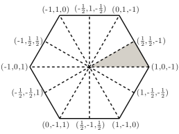
Figure 3.1: Symmetry under ${\mathcal{A}}_{2}$ (left), ${\mathcal{A}}_{2}^{*}$ (center) and $G_{2}$ (right) in the physical space. The shaded area is the fundamental triangle of $\Omega_{A}$ under $G_{2}$.

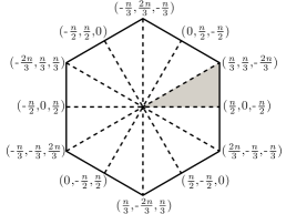
Figure 3.2: Symmetry under ${\mathcal{A}}_{2}$ (left), ${\mathcal{A}}_{2}^{*}$ (center) and $G_{2}$ (right) in the frequency space. The shaded area is the fundamental triangle of $\Omega_{B}$ under $G_{2}$.

For $\sigma\in G_{2}$, the number of inversion $|\sigma|$ satisfies $|-\sigma|=|\sigma|$. The following lemma can be easily verified (writing down the table of $\sigma\sigma^{*}$ for $\sigma\in A_{2}$ and $\sigma^{*}\in A_{2}^{*}$ if necessary).

Lemma 3.2.

Let $f$ be a generic H-periodic function. Then

$${\mathcal{P}}^{+}_{\!*}{\mathcal{P}}^{+}f({\mathbf{t}})=\frac{1}{12}\sum_{\sigma\in\mathcal{A}_{2}}\left(f({\mathbf{t}}\sigma)+f(-{\mathbf{t}}\sigma)\right)=\frac{1}{12}\sum_{\sigma\in\mathcal{G}_{2}}f({\mathbf{t}}\sigma),$$

$${\mathcal{P}}^{-}_{\!*}{\mathcal{P}}^{+}f({\mathbf{t}})=\frac{1}{12}\sum_{\sigma\in\mathcal{A}_{2}}\left(f({\mathbf{t}}\sigma)-f(-{\mathbf{t}}\sigma)\right)=\frac{1}{12}\sum_{\sigma\in\mathcal{A}_{2}^{*}}(-1)^{|\sigma|}\left(f({\mathbf{t}}\sigma)-f(-{\mathbf{t}}\sigma)\right),$$

$${\mathcal{P}}^{+}_{\!*}{\mathcal{P}}^{-}f({\mathbf{t}})=\frac{1}{12}\sum_{\sigma\in\mathcal{A}_{2}}(-1)^{|\sigma|}\left(f({\mathbf{t}}\sigma)-f(-{\mathbf{t}}\sigma)\right)=\frac{1}{12}\sum_{\sigma\in\mathcal{A}_{2}^{*}}\left(f({\mathbf{t}}\sigma)-f(-{\mathbf{t}}\sigma)\right),$$

$${\mathcal{P}}^{-}_{\!*}{\mathcal{P}}^{-}f({\mathbf{t}})=\frac{1}{12}\sum_{\sigma\in\mathcal{A}_{2}}(-1)^{|\sigma|}\left(f({\mathbf{t}}\sigma)+f(-{\mathbf{t}}\sigma)\right)=\frac{1}{12}\sum_{\sigma\in\mathcal{G}_{2}}(-1)^{|\sigma|}f({\mathbf{t}}\sigma).$$

For $\phi_{\mathbf{k}}({\mathbf{t}})=\mathrm{e}^{\frac{2\pi i{\mathbf{k}}\cdot{\mathbf{t}}}{3}}$, the action of ${\mathcal{P}}^{+}$ and ${\mathcal{P}}^{-}$ on $\phi_{\mathbf{k}}$ are called the generalized cosine and generalized sine functions in [9], which are trigonometric functions given by

$${\mathsf{C}}_{\mathbf{k}}({\mathbf{t}}):={\mathcal{P}}^{+}\phi_{\mathbf{k}}({\mathbf{t}})=\frac{1}{3}\left[\mathrm{e}^{\frac{i\pi}{3}(k_{1}-k_{3})(t_{1}-t_{3})}\cos k_{2}\pi t_{2}\right.$$

$$\left.\hphantom{{\mathsf{C}}_{\mathbf{k}}({\mathbf{t}}):={\mathcal{P}}^{+}\phi_{\mathbf{k}}({\mathbf{t}})=}{}+\mathrm{e}^{\frac{i\pi}{3}(k_{1}-k_{3})(t_{2}-t_{1})}\cos k_{2}\pi t_{3}+\mathrm{e}^{\frac{i\pi}{3}(k_{1}-k_{3})(t_{3}-t_{2})}\cos k_{2}\pi t_{1}\right],$$ (3.3)

$${\mathsf{S}}_{\mathbf{k}}({\mathbf{t}}):=\frac{1}{i}{\mathcal{P}}^{-}\phi_{\mathbf{k}}({\mathbf{t}})=\frac{1}{3}\left[\mathrm{e}^{\frac{i\pi}{3}(k_{1}-k_{3})(t_{1}-t_{3})}\sin k_{2}\pi t_{2}\right.$$

$$\left.\hphantom{{\mathsf{S}}_{\mathbf{k}}({\mathbf{t}}):=\frac{1}{i}{\mathcal{P}}^{-}\phi_{\mathbf{k}}({\mathbf{t}})=}{}+\mathrm{e}^{\frac{i\pi}{3}(k_{1}-k_{3})(t_{2}-t_{1})}\sin k_{2}\pi t_{3}+\mathrm{e}^{\frac{i\pi}{3}(k_{1}-k_{3})(t_{3}-t_{2})}\sin k_{2}\pi t_{1}\right].$$ (3.4)

Because of the symmetry, we only need to consider these functions on the fundamental domain of the group ${\mathcal{A}}_{2}$, which is one of the equilateral triangles of the regular hexagon. These functions form a complete orthogonal basis on the equilateral triangle and they are the analogues of the cosine and sine functions on the equilateral triangle. These generalized cosine and sine functions are the building blocks of the discrete Fourier analysis on the equilateral triangle and subsequent analysis of generalized Chebyshev polynomials in [9].

We now define the analogue of such functions on $G_{2}$. Since the fundamental domain of the group $G_{2}$ is the $30^{\degree}$–$60^{\degree}$–$90^{\degree}$ triangle, which is half of the equilateral triangle, we can relate the new functions to the generalized cosine and sine functions on the latter domain. There are, however, four families of such functions, defined as follows:

$${\mathsf{CC}}_{\mathbf{k}}({\mathbf{t}}):={\mathcal{P}}_{\!*}^{+}{\mathcal{P}}^{+}\phi_{\mathbf{k}}({\mathbf{t}})=\frac{1}{12}\sum_{\sigma\in\mathcal{A}_{2}}\left(\phi_{{\mathbf{k}}\sigma}({\mathbf{t}})+\phi_{-{\mathbf{k}}\sigma}({\mathbf{t}})\right)=\frac{1}{2}\big{(}{\mathsf{C}}_{\mathbf{k}}({\mathbf{t}})+{\mathsf{C}}_{-{\mathbf{k}}}({\mathbf{t}})\big{)},$$

$${\mathsf{SC}}_{\mathbf{k}}({\mathbf{t}}):=\frac{1}{i}{\mathcal{P}}_{\!*}^{-}{\mathcal{P}}^{+}\phi_{\mathbf{k}}({\mathbf{t}})=\frac{1}{12i}\sum_{\sigma\in\mathcal{A}_{2}}\left(\phi_{{\mathbf{k}}\sigma}({\mathbf{t}})-\phi_{-{\mathbf{k}}\sigma}({\mathbf{t}})\right)=\frac{1}{2i}\big{(}{\mathsf{C}}_{\mathbf{k}}({\mathbf{t}})-{\mathsf{C}}_{-{\mathbf{k}}}({\mathbf{t}})\big{)},$$

$${\mathsf{CS}}_{\mathbf{k}}({\mathbf{t}}):=\frac{1}{i}{\mathcal{P}}_{\!*}^{+}{\mathcal{P}}^{-}\phi_{\mathbf{k}}({\mathbf{t}})=\frac{1}{12i}\sum_{\sigma\in\mathcal{A}_{2}}(-1)^{|\sigma|}\left(\phi_{{\mathbf{k}}\sigma}({\mathbf{t}})-\phi_{-{\mathbf{k}}\sigma}({\mathbf{t}})\right)=\frac{1}{2}\big{(}{\mathsf{S}}_{\mathbf{k}}({\mathbf{t}})-{\mathsf{S}}_{-{\mathbf{k}}}({\mathbf{t}})\big{)},$$

$${\mathsf{SS}}_{\mathbf{k}}({\mathbf{t}}):=-{\mathcal{P}}_{\!*}^{-}{\mathcal{P}}^{-}\phi_{\mathbf{k}}({\mathbf{t}})=-\frac{1}{12}\sum_{\sigma\in\mathcal{A}_{2}}(-1)^{|\sigma|}\left(\phi_{{\mathbf{k}}\sigma}({\mathbf{t}})+\phi_{-{\mathbf{k}}\sigma}({\mathbf{t}})\right)=\frac{1}{2i}\big{(}{\mathsf{S}}_{\mathbf{k}}({\mathbf{t}})+{\mathsf{S}}_{-{\mathbf{k}}}({\mathbf{t}})\big{)},$$

where the second and the third equalities follow directly from the definition. We call these functions generalized trigonometric functions. As their names indicate, they are of the mixed type of cosine and sine functions.

From (3.3) and (3.4), we can derive explicit formulas for these functions, which are

$${\mathsf{CC}}_{\mathbf{k}}({\mathbf{t}})=\frac{1}{3}\Big{[}\cos{\tfrac{\pi(k_{1}-k_{3})(t_{1}-t_{3})}{3}}\cos\pi k_{2}t_{2}+\cos{\tfrac{\pi(k_{1}-k_{3})(t_{2}-t_{1})}{3}}\cos\pi k_{2}t_{3}$$

$$\hphantom{{\mathsf{CC}}_{\mathbf{k}}({\mathbf{t}})=}{}+\cos{\tfrac{\pi(k_{1}-k_{3})(t_{3}-t_{2})}{3}}\cos\pi k_{2}t_{1}\Big{]},$$ (3.5)

$${\mathsf{SC}}_{\mathbf{k}}({\mathbf{t}})=\frac{1}{3}\Big{[}\sin{\tfrac{\pi(k_{1}-k_{3})(t_{1}-t_{3})}{3}}\cos\pi k_{2}t_{2}+\sin{\tfrac{\pi(k_{1}-k_{3})(t_{2}-t_{1})}{3}}\cos\pi k_{2}t_{3}$$

$$\hphantom{{\mathsf{SC}}_{\mathbf{k}}({\mathbf{t}})=}{}+\sin{\tfrac{\pi(k_{1}-k_{3})(t_{3}-t_{2})}{3}}\cos\pi k_{2}t_{1}\Big{]},$$ (3.6)

$${\mathsf{CS}}_{\mathbf{k}}({\mathbf{t}})=\frac{1}{3}\Big{[}\cos{\tfrac{\pi(k_{1}-k_{3})(t_{1}-t_{3})}{3}}\sin\pi k_{2}t_{2}+\cos{\tfrac{\pi(k_{1}-k_{3})(t_{2}-t_{1})}{3}}\sin\pi k_{2}t_{3}$$

$$\hphantom{{\mathsf{CS}}_{\mathbf{k}}({\mathbf{t}})=}{}+\cos{\tfrac{\pi(k_{1}-k_{3})(t_{3}-t_{2})}{3}}\sin\pi k_{2}t_{1}\Big{]},$$ (3.7)

$${\mathsf{SS}}_{\mathbf{k}}({\mathbf{t}})=\frac{1}{3}\Big{[}\sin{\tfrac{\pi(k_{1}-k_{3})(t_{1}-t_{3})}{3}}\sin\pi k_{2}t_{2}+\sin{\tfrac{\pi(k_{1}-k_{3})(t_{2}-t_{1})}{3}}\sin\pi k_{2}t_{3}$$

$$\hphantom{{\mathsf{SS}}_{\mathbf{k}}({\mathbf{t}})=}{}+\sin{\tfrac{\pi(k_{1}-k_{3})(t_{3}-t_{2})}{3}}\sin\pi k_{2}t_{1}\Big{]}.$$ (3.8)

In particular, it follows from (3.6)–(3.8) that ${\mathsf{CS}}_{\mathbf{k}}({\mathbf{t}})\equiv{\mathsf{SS}}_{\mathbf{k}}({\mathbf{t}})\equiv 0$ whenever ${\mathbf{k}}$ contains zero component and ${\mathsf{SC}}_{\mathbf{k}}({\mathbf{t}})\equiv{\mathsf{SS}}_{\mathbf{k}}({\mathbf{t}})\equiv 0$ whenever ${\mathbf{k}}$ contains equal elements. Similar formulas can be derived from the permutations of $t_{1}$, $t_{2}$, $t_{3}$. In fact, the functions ${\mathsf{CC}}_{\mathbf{k}}$ and ${\mathsf{SS}}_{\mathbf{k}}$ are invariant and anti-invariant under $G_{2}$, respectively, whereas the functions ${\mathsf{CS}}_{\mathbf{k}}$ and ${\mathsf{SC}}_{\mathbf{k}}$ are of the mixed type, with the first one invariant under ${\mathcal{A}}_{2}$ and anti-invariant under ${\mathcal{A}}_{2}^{*}$ and the second one invariant under ${\mathcal{A}}_{2}^{*}$ and anti-invariant under ${\mathcal{A}}_{2}$. More precisely, these invariant properties lead to the following identities:

$${\mathsf{CC}}_{\mathbf{k}}({\mathbf{t}}\sigma)={\mathsf{CC}}_{\mathbf{k}}({\mathbf{t}}),\qquad{\mathsf{SS}}_{\mathbf{k}}({\mathbf{t}}\sigma)=(-1)^{|\sigma|}{\mathsf{SS}}_{\mathbf{k}}({\mathbf{t}}),\qquad \sigma\in{\mathcal{G}}_{2},$$ (3.9)

$${\mathsf{SC}}_{\mathbf{k}}({\mathbf{t}}\sigma)=-{\mathsf{SC}}_{\mathbf{k}}(-{\mathbf{t}}\sigma)={\mathsf{SC}}_{\mathbf{k}}({\mathbf{t}}), \sigma\in{\mathcal{A}}_{2},$$ (3.10)

$${\mathsf{CS}}_{\mathbf{k}}({\mathbf{t}}\sigma)=-{\mathsf{CS}}_{\mathbf{k}}(-{\mathbf{t}}\sigma)=(-1)^{|\sigma|}{\mathsf{CS}}_{\mathbf{k}}({\mathbf{t}}), \sigma\in{\mathcal{A}}_{2},$$ (3.11)

$${\mathsf{SC}}_{\mathbf{k}}({\mathbf{t}}\sigma)=-{\mathsf{SC}}_{\mathbf{k}}(-{\mathbf{t}}\sigma)=(-1)^{|\sigma|}{\mathsf{SC}}_{\mathbf{k}}({\mathbf{t}}), \sigma\in{\mathcal{A}}_{2}^{*},$$ (3.12)

$${\mathsf{CS}}_{\mathbf{k}}({\mathbf{t}}\sigma)=-{\mathsf{CS}}_{\mathbf{k}}(-{\mathbf{t}}\sigma)={\mathsf{CS}}_{\mathbf{k}}({\mathbf{t}}), \sigma\in{\mathcal{A}}_{2}^{*}.$$ (3.13)

In particular, it follows from (3.6)–(3.8) that ${\mathsf{CS}}_{\mathbf{k}}({\mathbf{t}})\equiv{\mathsf{SS}}_{\mathbf{k}}({\mathbf{t}})\equiv 0$ whenever ${\mathbf{k}}$ contains zero component and ${\mathsf{SC}}_{\mathbf{k}}({\mathbf{t}})\equiv{\mathsf{SS}}_{\mathbf{k}}({\mathbf{t}})\equiv 0$ whenever ${\mathbf{k}}$ contains equal elements. Moreover, for any ${\mathbf{k}}\in{\mathbb{H}}^{{\dagger}}$, ${\mathsf{CS}}_{\mathbf{k}}({\mathbf{t}})={\mathsf{SS}}_{\mathbf{k}}({\mathbf{t}})=0$ whenever ${\mathbf{t}}$ contains zero component and ${\mathsf{SC}}_{\mathbf{k}}({\mathbf{t}})={\mathsf{SS}}_{\mathbf{k}}({\mathbf{t}})=0$ whenever ${\mathbf{t}}$ contains equal elements.

Because of their invariant properties, we only need to consider these functions on one of the twelve $30^{{\degree}}$–$60^{{\degree}}$–$90^{{\degree}}$ triangles in the hexagon $\Omega$. We shall choose the triangle as

$$\triangle:=\{{\mathbf{t}}\in{\mathbb{R}}_{H}^{3}:0\leq t_{2}\leq t_{1}\leq-t_{3}\leq 1\}.$$ (3.14)

The region $\triangle$ and its relative position in the hexagon are depicted in Figs. 3.3 and 3.1.

Figure 3.3: The fundamental triangles in $\Omega_{A}$ (left) and $\Omega_{B}$ (right).

When ${\mathsf{CC}}_{\mathbf{k}}$, ${\mathsf{SC}}_{\mathbf{k}}$, ${\mathsf{CS}}_{\mathbf{k}}$, ${\mathsf{SS}}_{\mathbf{k}}$ are restricted to the triangle $\triangle$, we only need to consider a subset of ${\mathbf{k}}\in{\mathbb{H}}^{{\dagger}}$ as can be seen by the relations in (3.9)–(3.13). Indeed, we can restrict ${\mathbf{k}}$ to the index sets

$$\Gamma=\Gamma^{\operatorname{cc}}:=\big{\{}{\mathbf{k}}\in{\mathbb{H}}^{{\dagger}}:\;0\leq k_{2}\leq k_{1}\big{\}},\qquad\Gamma^{\operatorname{sc}}:=\big{\{}{\mathbf{k}}\in{\mathbb{H}}^{{\dagger}}:\;0\leq k_{2}<k_{1}\big{\}},$$ (3.15)

$$\hphantom{\Gamma=}{}\ \Gamma^{\operatorname{cs}}:=\big{\{}{\mathbf{k}}\in{\mathbb{H}}^{{\dagger}}:\;0<k_{2}\leq k_{1}\big{\}},\qquad\Gamma^{\operatorname{ss}}:=\big{\{}{\mathbf{k}}\in{\mathbb{H}}^{{\dagger}}:\;0<k_{2}<k_{1}\big{\}},$$ (3.16)

respectively, where the notation is self-explanatory; for example, $\Gamma^{\operatorname{cc}}$ is the index set for ${\mathsf{CC}}_{\mathbf{k}}$. We define an inner product on $\triangle$ by

$$\langle f,g\rangle_{\triangle}:=\frac{1}{|\triangle|}\int_{\triangle}f({\mathbf{t}})\overline{g({\mathbf{t}})}d{\mathbf{t}}=4\int_{0}^{\frac{1}{2}}dt_{2}\int_{t_{2}}^{1-t_{2}}f({\mathbf{t}})\overline{g({\mathbf{t}})}dt_{1}.$$

If $f\bar{g}$ is invariant under the group $G_{2}$, then it is easy to see that $\langle f,g\rangle_{\Omega}=\langle f,g\rangle_{\triangle}$. Consequently, we can deduce the orthogonality of ${\mathsf{CC}}_{\mathbf{k}}$, ${\mathsf{SC}}_{\mathbf{k}}$, ${\mathsf{CS}}_{\mathbf{k}}$, ${\mathsf{SS}}_{\mathbf{k}}$ from that of $\phi_{\mathbf{k}}$ on $\Omega$.

Proposition 3.3.

It holds that

$$\langle{\mathsf{CC}}_{\mathbf{k}},{\mathsf{CC}}_{{\mathbf{j}}}\rangle_{\triangle}=\frac{\triangle_{{\mathbf{k}},{\mathbf{j}}}}{|{\mathbf{k}}G_{2}|}=\triangle_{{\mathbf{k}},{\mathbf{j}}}\begin{cases}1,&{\mathbf{k}}=0,\\ \frac{1}{6},&k_{2}(k_{1}-k_{2})=0,\,k_{1}>0,\\ \frac{1}{12},&k_{1}>k_{2}>0,\end{cases}\qquad {\mathbf{j}},{\mathbf{k}}\in\Gamma^{\operatorname{cc}},$$ (3.17)

$$\langle{\mathsf{SC}}_{\mathbf{k}},{\mathsf{SC}}_{{\mathbf{j}}}\rangle_{\triangle}=\frac{\triangle_{{\mathbf{k}},{\mathbf{j}}}}{|{\mathbf{k}}G_{2}|}=\triangle_{{\mathbf{k}},{\mathbf{j}}}\begin{cases}\frac{1}{6},&k_{2}=0,\\ \frac{1}{12},&k_{1}>k_{2}>0,\end{cases} {\mathbf{j}},{\mathbf{k}}\in\Gamma^{\operatorname{sc}},$$ (3.18)

$$\langle{\mathsf{CS}}_{\mathbf{k}},{\mathsf{CS}}_{{\mathbf{j}}}\rangle_{\triangle}=\frac{\triangle_{{\mathbf{k}},{\mathbf{j}}}}{|{\mathbf{k}}G_{2}|}=\triangle_{{\mathbf{k}},{\mathbf{j}}}\begin{cases}\frac{1}{6},&k_{1}=k_{2}>0,\\ \frac{1}{12},&k_{1}>k_{2}>0,\end{cases} {\mathbf{j}},{\mathbf{k}}\in\Gamma^{\operatorname{cs}},$$ (3.19)

$$\langle{\mathsf{SS}}_{\mathbf{k}},{\mathsf{SS}}_{{\mathbf{j}}}\rangle_{\triangle}=\frac{\triangle_{{\mathbf{k}},{\mathbf{j}}}}{|{\mathbf{k}}G_{2}|}=\tfrac{1}{12}\triangle_{{\mathbf{k}},{\mathbf{j}}}, {\mathbf{j}},{\mathbf{k}}\in\Gamma^{\operatorname{ss}},$$ (3.20)

where ${\mathbf{k}}G_{2}=\left\{{\mathbf{k}}\sigma:\sigma\in G_{2}\right\}$ denotes the orbit of ${\mathbf{k}}$ under $G_{2}$.

3.2 Discrete Fourier analysis on the $\boldsymbol{30^{{\degree}}}$–$\boldsymbol{60^{{\degree}}}$–$\boldsymbol{90^{{\degree}}}$ triangle

Using the fact that ${\mathsf{CC}}_{\mathbf{k}}$, ${\mathsf{SC}}_{{\mathbf{k}}}$ and ${\mathsf{CS}}_{\mathbf{k}}$, ${\mathsf{SS}}_{\mathbf{k}}$ are invariant and anti-invariant under ${\mathcal{A}}_{2}$ and that ${\mathsf{CC}}_{\mathbf{k}}$, ${\mathsf{CS}}_{{\mathbf{k}}}$ and ${\mathsf{SC}}_{\mathbf{k}}$, ${\mathsf{SS}}_{\mathbf{k}}$ are invariant and anti-invariant under ${\mathcal{A}}_{2}^{*}$, we can deduce a discrete orthogonality for the generalized trignometric functions. Again, we state the main result in terms of cubature rules. The index set for the nodes of the cubature rule is given by

$$\Upsilon_{n}:=\left\{{\mathbf{j}}\in{\mathbb{H}}:\;0\leq j_{2}\leq j_{1}\leq-j_{3}\leq n\right\},$$

which are located inside $n\triangle$ as seen by (3.14). The space of invariant functions being integrated exactly by the cubature rule are indexed by

$$\Gamma_{n}=\Gamma_{n}^{\operatorname{cc}}:=\Gamma\cup{\mathbb{H}}^{{\dagger}}_{n}=\big{\{}{\mathbf{k}}\in{\mathbb{H}}^{{\dagger}}:\,0\leq k_{2}\leq k_{1}\leq k_{3}+n\big{\}},$$

$$\hphantom{\Gamma_{n}=}{}\ \Gamma_{n}^{\operatorname{sc}}:=\Gamma^{\operatorname{sc}}\cup{\mathbb{H}}^{{\dagger}}_{n}=\big{\{}{\mathbf{k}}\in{\mathbb{H}}^{{\dagger}}:\,0\leq k_{2}<k_{1}<k_{3}+n\big{\}},$$

$$\hphantom{\Gamma_{n}=}{}\ \Gamma_{n}^{\operatorname{cs}}:=\Gamma^{\operatorname{cs}}\cup{\mathbb{H}}^{{\dagger}}_{n}=\big{\{}{\mathbf{k}}\in{\mathbb{H}}^{{\dagger}}:\,0<k_{2}\leq k_{1}\leq k_{3}+n\big{\}},$$

$$\hphantom{\Gamma_{n}=}{}\ \Gamma_{n}^{\operatorname{ss}}:=\Gamma^{\operatorname{ss}}\cup{\mathbb{H}}^{{\dagger}}_{n}=\big{\{}{\mathbf{k}}\in{\mathbb{H}}^{{\dagger}}:\,0<k_{2}<k_{1}<k_{3}+n\big{\}}.$$

Correspondingly, we define the following subspaces of ${\mathcal{H}}_{n}^{{\dagger}}$,

$${\mathcal{H}}^{\operatorname{cc}}_{n}:=\operatorname{span}\{{\mathsf{CC}}_{\mathbf{k}}:{\mathbf{k}}\in\Gamma_{n}^{\operatorname{cc}}\},\qquad{\mathcal{H}}^{\operatorname{sc}}_{n}:=\operatorname{span}\{{\mathsf{SC}}_{\mathbf{k}}:{\mathbf{k}}\in\Gamma_{n}^{\operatorname{sc}}\},$$

$${\mathcal{H}}^{\operatorname{cs}}_{n}:=\operatorname{span}\{{\mathsf{CS}}_{\mathbf{k}}:{\mathbf{k}}\in\Gamma_{n}^{\operatorname{cs}}\},\qquad{\mathcal{H}}^{\operatorname{ss}}_{n}:=\operatorname{span}\{{\mathsf{SS}}_{\mathbf{k}}:{\mathbf{k}}\in\Gamma_{n}^{\operatorname{ss}}\}.$$

It is easy to verify that

$$\dim{\mathcal{H}}^{\operatorname{cc}}_{n}=|\Gamma_{n}^{\operatorname{cc}}|=\tfrac{1}{2}\big{(}3\lfloor\tfrac{n}{3}\rfloor-2n\big{)}\big{(}\lfloor\tfrac{n}{3}\rfloor+1\big{)}-\big{(}\lfloor\tfrac{n}{2}\rfloor-n-1\big{)}\big{(}\lfloor\tfrac{n}{2}\rfloor+1\big{)},$$

$$\dim{\mathcal{H}}^{\operatorname{ss}}_{n}=|\Gamma_{n}^{\operatorname{ss}}|=|\Gamma_{n-6}|,\qquad\dim{\mathcal{H}}^{\operatorname{sc}}_{n}=|\Gamma_{n}^{\operatorname{sc}}|=\dim{\mathcal{H}}^{\operatorname{cs}}_{n}=|\Gamma_{n}^{\operatorname{cs}}|=|\Gamma_{n-3}|.$$ (3.21)

Figure 3.4: The index set $\Upsilon_{n}$. $n\equiv 0\pmod{3}$ (left), $n\equiv 1\pmod{3}$ (center) and $n\equiv 2\pmod{3}$ (right).

(cc) (sc)

(cs) (ss)

Figure 3.5: The index set $\Gamma_{n}$.

Theorem 3.4.

The following cubature is exact for all $f\in{\mathcal{H}}^{\operatorname{cc}}_{2n-1}$

$$\frac{1}{|\triangle|}\int_{\triangle}f({\mathbf{t}})d{\mathbf{t}}=\frac{1}{n^{2}}\sum_{{\mathbf{j}}\in\Upsilon_{n}}\omega_{{\mathbf{j}}}^{(n)}f\left(\frac{{\mathbf{j}}}{n}\right),$$ (3.22)

where

$$\omega_{\mathbf{j}}^{(n)}:=c^{(n)}_{{\mathbf{j}}}|{\mathbf{j}}G_{2}|=\left\{\begin{array}[]{lll}12,&{\mathbf{j}}\in\Upsilon^{{\degree}}_{n},&(\text{interior}),\\[1.99997pt] 1,&{\mathbf{j}}=\mathbf{0},&(30^{{\degree}}\text{-vertex}),\\[1.99997pt] 2,&{\mathbf{j}}=(n,0,-n),&(60^{{\degree}}\text{-vertex}),\\[1.99997pt] 3,&{\mathbf{j}}=(\frac{n}{2},\frac{n}{2},-n),&(90^{{\degree}}\text{-vertex}),\\[1.99997pt] 6,&\text{otherwise},&(\text{boundaries}).\end{array}\right.$$

Moreover, if we define the discrete inner product $\langle f,g\rangle_{\triangle,n}=\frac{1}{n^{2}}\sum\limits_{{\mathbf{j}}\in\Upsilon_{n}}\omega_{{\mathbf{j}}}^{(n)}f(\frac{{\mathbf{j}}}{n})\overline{g(\frac{{\mathbf{j}}}{n})}$, then

$$\langle{\mathsf{CC}}_{{\mathbf{j}}},{\mathsf{CC}}_{{\mathbf{k}}}\rangle_{\triangle,n}=\frac{\triangle_{{\mathbf{j}},{\mathbf{k}}}}{c^{(n)}_{\widehat{{\mathbf{k}}}}|{\mathbf{k}}G_{2}|}=\frac{\triangle_{{\mathbf{j}},{\mathbf{k}}}}{\omega^{(n)}_{\widehat{{\mathbf{k}}}}},\qquad {\mathbf{j}},{\mathbf{k}}\in\Gamma_{n},$$

$$\langle{\mathsf{SC}}_{{\mathbf{j}}},{\mathsf{SC}}_{{\mathbf{k}}}\rangle_{\triangle,n}=\frac{\triangle_{{\mathbf{j}},{\mathbf{k}}}}{c^{(n)}_{\widehat{{\mathbf{k}}}}|{\mathbf{k}}G_{2}|}=\frac{\triangle_{{\mathbf{j}},{\mathbf{k}}}}{\omega^{(n)}_{\widehat{{\mathbf{k}}}}},\qquad {\mathbf{j}},{\mathbf{k}}\in\Gamma^{\operatorname{sc}}_{n},$$

$$\langle{\mathsf{CS}}_{{\mathbf{j}}},{\mathsf{CS}}_{{\mathbf{k}}}\rangle_{\triangle,n}=\frac{\triangle_{{\mathbf{j}},{\mathbf{k}}}}{c^{(n)}_{\widehat{{\mathbf{k}}}}|{\mathbf{k}}G_{2}|}=\frac{\triangle_{{\mathbf{j}},{\mathbf{k}}}}{\omega^{(n)}_{\widehat{{\mathbf{k}}}}},\qquad {\mathbf{j}},{\mathbf{k}}\in\Gamma^{\operatorname{cs}}_{n},$$

$$\langle{\mathsf{SS}}_{{\mathbf{j}}},{\mathsf{SS}}_{{\mathbf{k}}}\rangle_{\triangle,n}=\frac{\triangle_{{\mathbf{j}},{\mathbf{k}}}}{c^{(n)}_{\widehat{{\mathbf{k}}}}|{\mathbf{k}}G_{2}|}=\frac{\triangle_{{\mathbf{j}},{\mathbf{k}}}}{12},\qquad {\mathbf{j}},{\mathbf{k}}\in\Gamma^{\operatorname{ss}}_{n},$$

where $\widehat{\mathbf{k}}=(k_{3}-k_{2},k_{1}-k_{3},k_{2}-k_{1})$.

The formula (3.22) is derived from (2.4) by using the invariance of the functions in ${\mathcal{H}}^{\operatorname{cc}}_{2n-1}$ and upon writing $\Omega=\big{(}\bigcup_{\sigma\in G_{2}}\{{\mathbf{t}}\sigma:{\mathbf{t}}\in\triangle^{{\degree}}\}\big{)}\bigcup\big{(}\bigcup_{\sigma\in G_{2}}\{{\mathbf{t}}\sigma:{\mathbf{t}}\in\partial\triangle\}\big{)}$. The reason that $\widehat{\mathbf{k}}$ appears goes back to Proposition 2.3. As the proof is similar to that in [9], we shall omit the details.

One may note that the formulation of the result resembles a Gaussian quadrature. The connection will be discussed in Section 6.

3.3 Sturm–Liouville eigenvalue problem for the Laplace operator

Recall the relation (2.3) between the coordinates $(x_{1},x_{2})$ and the homogeneous coordinates $(t_{1},t_{2},t_{3})$. A quick calculation gives the expression of the Laplace operator in homogeneous coordinates,

$$\Delta:=\frac{\partial^{2}}{\partial x_{1}^{2}}+\frac{\partial^{2}}{\partial x_{2}^{2}}=\frac{1}{2}\left[\left(\frac{\partial}{\partial t_{1}}-\frac{\partial}{\partial t_{2}}\right)^{2}+\left(\frac{\partial}{\partial t_{2}}-\frac{\partial}{\partial t_{3}}\right)^{2}+\left(\frac{\partial}{\partial t_{3}}-\frac{\partial}{\partial t_{1}}\right)^{2}\right].$$

A further computation shows that $\phi_{\mathbf{k}}({\mathbf{t}})=\mathrm{e}^{\frac{2\pi i}{3}{\mathbf{k}}\cdot{\mathbf{t}}}$ are the eigenfunctions of the Laplace operator: for ${\mathbf{k}}\in{\mathbb{H}}$,

$$\Delta\phi_{\mathbf{k}}=-\lambda_{\mathbf{k}}\phi_{\mathbf{k}},\qquad\lambda_{\mathbf{k}}:=\frac{2\pi^{2}}{9}\left[(k_{1}-k_{2})^{2}+(k_{2}-k_{3})^{2}+(k_{3}-k_{1})^{2}\right].$$ (3.23)

As a consequence, our generalized trigonometric functions are the solutions of the Sturm–Liouville eigenvalue problem for the Laplace operator with certain boundary conditions on the $30^{\degree}$–$60^{\degree}$–$90^{\degree}$ triangle. To be more precise, we denote the three linear segments that are the boundary of this triangle by $B_{1}$, $B_{2}$, $B_{3}$,

$$B_{1}:=\{{\mathbf{t}}\in\triangle:t_{3}=-1\},\qquad B_{2}:=\{{\mathbf{t}}\in\triangle:t_{2}=0\},\qquad B_{3}:=\{{\mathbf{t}}\in\triangle:t_{1}=t_{2}\}.$$

Let $\frac{\partial}{\partial n}$ denote the partial derivative in the direction of the exterior norm of $\triangle$. Then

$$\frac{\partial}{\partial n}\Big{|}_{B_{1}}=-\frac{\partial}{\partial t_{3}},\qquad\frac{\partial}{\partial n}\Big{|}_{B_{2}}=-\frac{\partial}{\partial t_{2}},\qquad\frac{\partial}{\partial n}\Big{|}_{B_{1}}=\frac{\partial}{\partial t_{2}}-\frac{\partial}{\partial t_{1}}.$$

Theorem 3.5.

The generalized trigonometric functions ${\mathsf{CC}}_{\mathbf{k}}$, ${\mathsf{SC}}_{\mathbf{k}}$, ${\mathsf{CS}}_{\mathbf{k}}$, ${\mathsf{SS}}_{\mathbf{k}}$ are the eigenfunctions of the Laplace operator, $\Delta u=-\lambda_{\mathbf{k}}u$, that satisfy the boundary conditions:

$${\mathsf{CC}}_{\mathbf{k}}:\ \frac{\partial u}{\partial n}\Big{|}_{B_{1}\cup B_{2}\cup B_{3}}=0,\qquad {\mathsf{SC}}_{\mathbf{k}}:\ \frac{\partial u}{\partial n}\Big{|}_{B_{1}\cup B_{2}}=0,\qquad u|_{B_{3}}=0,$$

$${\mathsf{CS}}_{\mathbf{k}}:\ \frac{\partial u}{\partial n}\Big{|}_{B_{3}}=0,\qquad u|_{B_{1}\cup B_{2}}=0,\qquad {\mathsf{SS}}_{\mathbf{k}}:\ u|_{B_{1}\cup B_{2}\cup B_{3}}=0.$$

Proof.

Since $\lambda_{\mathbf{k}}$ is invariant under $G_{2}$, that is, $\lambda_{\mathbf{k}}=\lambda_{{\mathbf{k}}\sigma}$, $\forall\,\sigma\in G_{2}$, that these functions satisfy $\Delta u=-\lambda_{\mathbf{k}}u$ follows directly from their definitions. The boundary conditions can be verified directly via the equations (3.5), (3.6), (3.7) and (3.8). ∎

In particular, ${\mathsf{CC}}_{\mathbf{k}}$ satisfies the Neumann boundary conditions and ${\mathsf{SS}}_{\mathbf{k}}$ satisfies the Dirichlet type boundary conditions.

3.4 Product formulas for the generalized trigonometric functions

Below we give a list of identities on the product of the generalized trigonometric functions, which will be needed in the following section.

Lemma 3.6.

The generalized trigonometric functions satisfy the relations,

$${\mathsf{CC}}_{{\mathbf{j}}}{\mathsf{CC}}_{{\mathbf{k}}}=\frac{1}{12}\sum_{\sigma\in G_{2}}{\mathsf{CC}}_{{\mathbf{k}}+{\mathbf{j}}\sigma}=\frac{1}{12}\sum_{\sigma\in G_{2}}{\mathsf{CC}}_{{\mathbf{j}}+{\mathbf{k}}\sigma},$$ (3.24)

$${\mathsf{CC}}_{{\mathbf{j}}}{\mathsf{SC}}_{{\mathbf{k}}}=\frac{1}{12}\sum_{\sigma\in G_{2}}{\mathsf{SC}}_{{\mathbf{k}}+{\mathbf{j}}\sigma}=\frac{1}{12}\sum_{\tau\in{\mathcal{A}}_{2}^{*}}(-1)^{\tau}\big{(}{\mathsf{SC}}_{{\mathbf{j}}+{\mathbf{k}}\tau}-{\mathsf{SC}}_{{\mathbf{j}}-{\mathbf{k}}\tau}\big{)},$$ (3.25)

$${\mathsf{CC}}_{{\mathbf{j}}}{\mathsf{CS}}_{{\mathbf{k}}}=\frac{1}{12}\sum_{\sigma\in G_{2}}{\mathsf{CS}}_{{\mathbf{k}}+{\mathbf{j}}\sigma}=\frac{1}{12}\sum_{\tau\in{\mathcal{A}}_{2}^{*}}\big{(}{\mathsf{CS}}_{{\mathbf{j}}+{\mathbf{k}}\tau}-{\mathsf{CS}}_{{\mathbf{j}}-{\mathbf{k}}\tau}\big{)},$$ (3.26)

$${\mathsf{CC}}_{{\mathbf{j}}}{\mathsf{SS}}_{{\mathbf{k}}}=\frac{1}{12}\sum_{\sigma\in G_{2}}{\mathsf{SS}}_{{\mathbf{k}}+{\mathbf{j}}\sigma}=\frac{1}{12}\sum_{\sigma\in G_{2}}(-1)^{|\tau|}{\mathsf{SS}}_{{\mathbf{j}}+{\mathbf{k}}\sigma},$$ (3.27)

$${\mathsf{SC}}_{{\mathbf{j}}}{\mathsf{SC}}_{{\mathbf{k}}}=-\frac{1}{12}\sum_{\tau\in{\mathcal{A}}_{2}^{*}}(-1)^{|\tau|}\big{(}{\mathsf{CC}}_{{\mathbf{k}}+{\mathbf{j}}\tau}-{\mathsf{CC}}_{{\mathbf{k}}-{\mathbf{j}}\tau}\big{)}$$

$$\hphantom{{\mathsf{SC}}_{{\mathbf{j}}}{\mathsf{SC}}_{{\mathbf{k}}}}{}=-\frac{1}{12}\sum_{\tau\in{\mathcal{A}}_{2}^{*}}(-1)^{|\tau|}\big{(}{\mathsf{CC}}_{{\mathbf{j}}+{\mathbf{k}}\tau}-{\mathsf{CC}}_{{\mathbf{j}}-{\mathbf{k}}\tau}\big{)},$$ (3.28)

$${\mathsf{SC}}_{{\mathbf{j}}}{\mathsf{CS}}_{{\mathbf{k}}}=\frac{1}{12}\sum_{\tau\in{\mathcal{A}}_{2}^{*}}(-1)^{|\tau|}\big{(}{\mathsf{SS}}_{{\mathbf{k}}+{\mathbf{j}}\tau}-{\mathsf{SS}}_{{\mathbf{k}}-{\mathbf{j}}\tau}\big{)}=\frac{1}{12}\sum_{\tau\in{\mathcal{A}}_{2}^{*}}\big{(}{\mathsf{SS}}_{{\mathbf{j}}+{\mathbf{k}}\tau}-{\mathsf{SS}}_{{\mathbf{j}}-{\mathbf{k}}\tau}\big{)},$$ (3.29)

$${\mathsf{CS}}_{{\mathbf{j}}}{\mathsf{CS}}_{{\mathbf{k}}}=-\frac{1}{12}\sum_{\tau\in{\mathcal{A}}_{2}^{*}}\big{(}{\mathsf{CC}}_{{\mathbf{k}}+{\mathbf{j}}\tau}-{\mathsf{CC}}_{{\mathbf{k}}-{\mathbf{j}}\tau}\big{)}=-\frac{1}{12}\sum_{\tau\in{\mathcal{A}}_{2}^{*}}\big{(}{\mathsf{CC}}_{{\mathbf{j}}+{\mathbf{k}}\tau}-{\mathsf{CC}}_{{\mathbf{j}}-{\mathbf{k}}\tau}\big{)},$$ (3.30)

$${\mathsf{SS}}_{{\mathbf{j}}}{\mathsf{SS}}_{{\mathbf{k}}}=\frac{1}{12}\sum_{\sigma\in G_{2}}(-1)^{|\sigma|}{\mathsf{CC}}_{{\mathbf{k}}+{\mathbf{j}}\sigma}=\frac{1}{12}\sum_{\sigma\in G_{2}}(-1)^{|\sigma|}{\mathsf{CC}}_{{\mathbf{j}}+{\mathbf{k}}\sigma}.$$ (3.31)

Furthermore, the following formulas hold:

$$3{\mathsf{SC}}_{1,0,-1}({\mathbf{t}}){\mathsf{CS}}_{1,1,-2}({\mathbf{t}})={\mathsf{SS}}_{2,1,-3}({\mathbf{t}}),$$ (3.32)

$$[{\mathsf{SC}}_{1,0,-1}({\mathbf{t}})]^{2}=\frac{1}{3}\big{[}1+2{\mathsf{CC}}_{1,1,-2}\big{]}-[{\mathsf{CC}}_{1,0,-1}]^{2},$$ (3.33)

$$[{\mathsf{CS}}_{1,1,-2}]^{2}+[{\mathsf{CC}}_{1,1,-2}]^{2}=\frac{1}{3}\big{[}1+2{\mathsf{CC}}_{3,0,-3}\big{]},$$ (3.34)

$$[{\mathsf{CC}}_{1,0,-1}]^{3}=\frac{1}{36}{\mathsf{CC}}_{3,0,-3}+\frac{1}{4}{\mathsf{CC}}_{1,0,-1}+\frac{1}{6}{\mathsf{CC}}_{1,1,-2}+\frac{1}{18}+\frac{1}{2}{\mathsf{CC}}_{1,1,-2}{\mathsf{CC}}_{1,0,-1}.$$ (3.35)

Proof.

For (3.24)–(3.31), we only prove (3.29). Other identities can be proved similarly. By the definition of the generalized trigonometric functions,

$${\mathsf{SC}}_{{\mathbf{j}}}{\mathsf{CS}}_{{\mathbf{k}}}=\frac{1}{12i}\sum_{\sigma\in{\mathcal{A}}_{2}^{*}}(-1)^{|\sigma|}\big{(}\phi_{{\mathbf{j}}\sigma}-\phi_{-{\mathbf{j}}\sigma}\big{)}\times\frac{1}{12i}\sum_{\tau\in{\mathcal{A}}_{2}^{*}}\big{(}\phi_{{\mathbf{k}}\tau}-\phi_{-{\mathbf{k}}\tau}\big{)}$$

$$\hphantom{{\mathsf{SC}}_{{\mathbf{j}}}{\mathsf{CS}}_{{\mathbf{k}}}}{}=-\frac{1}{12^{2}}\sum_{\tau\in{\mathcal{A}}_{2}^{*}}(-1)^{|\tau|}\sum_{\sigma\in{\mathcal{A}}_{2}^{*}}(-1)^{|\sigma\tau^{-1}|}\big{[}\phi_{({\mathbf{k}}+{\mathbf{j}}\sigma\tau^{-1})\tau}+\phi_{-({\mathbf{k}}+{\mathbf{j}}\sigma\tau^{-1})\tau}$$

$$\hphantom{{\mathsf{SC}}_{{\mathbf{j}}}{\mathsf{CS}}_{{\mathbf{k}}}=}{}-\phi_{({\mathbf{k}}-{\mathbf{j}}\sigma\tau^{-1})\tau}-\phi_{-({\mathbf{k}}-{\mathbf{j}}\sigma\tau^{-1})\tau}\big{]}$$

upon using the relation $(-1)^{|\tau|+|\sigma\tau^{-1}|}=(-1)^{|\sigma|}$, consequently,

$${\mathsf{SC}}_{{\mathbf{j}}}{\mathsf{CS}}_{{\mathbf{k}}}=-\frac{1}{12^{2}}\sum_{\sigma\in{\mathcal{A}}_{2}^{*}}(-1)^{|\sigma|}\sum_{\tau\in{\mathcal{A}}_{2}^{*}}(-1)^{|\tau|}\big{[}\phi_{({\mathbf{k}}+{\mathbf{j}}\sigma)\tau}+\phi_{-({\mathbf{k}}+{\mathbf{j}}\sigma)\tau}-\phi_{({\mathbf{k}}-{\mathbf{j}}\sigma)\tau}-\phi_{-({\mathbf{k}}-{\mathbf{j}}\sigma)\tau}\big{]}$$

$$\hphantom{{\mathsf{SC}}_{{\mathbf{j}}}{\mathsf{CS}}_{{\mathbf{k}}}}{}=\frac{1}{12}\sum_{\sigma\in{\mathcal{A}}_{2}^{*}}(-1)^{|\sigma|}\big{(}{\mathsf{SS}}_{{\mathbf{k}}+{\mathbf{j}}\sigma}-{\mathsf{SS}}_{{\mathbf{k}}-{\mathbf{j}}\sigma}\big{)},$$

proving the first equality in (3.29). Further by (3.9),

$$\frac{1}{12}\sum_{\sigma\in{\mathcal{A}}_{2}^{*}}(-1)^{|\sigma|}\big{(}{\mathsf{SS}}_{{\mathbf{k}}+{\mathbf{j}}\sigma}-{\mathsf{SS}}_{{\mathbf{k}}-{\mathbf{j}}\sigma}\big{)}=\frac{1}{12}\sum_{\sigma\in{\mathcal{A}}_{2}^{*}}\big{(}{\mathsf{SS}}_{{\mathbf{k}}\sigma^{-1}+{\mathbf{j}}}-{\mathsf{SS}}_{{\mathbf{k}}\sigma^{-1}-{\mathbf{j}}}\big{)}$$

$$\qquad{}=\frac{1}{12}\sum_{\sigma\in{\mathcal{A}}_{2}^{*}}\big{(}{\mathsf{SS}}_{{\mathbf{j}}+{\mathbf{k}}\sigma}-{\mathsf{SS}}_{{\mathbf{k}}\sigma-{\mathbf{j}}}\big{)}=\frac{1}{12}\sum_{\sigma\in{\mathcal{A}}_{2}^{*}}\big{(}{\mathsf{SS}}_{{\mathbf{j}}+{\mathbf{k}}\sigma}-{\mathsf{SS}}_{{\mathbf{j}}-{\mathbf{k}}\sigma}\big{)},$$

since ${\mathsf{SS}}_{{\mathbf{j}}}={\mathsf{SS}}_{-{\mathbf{j}}}$ by (3.5). This completes the proof of (3.29).

We now prove the relations (3.32)–(3.35). By (3.29),

$${\mathsf{CS}}_{1,1,-2}({\mathbf{t}}){\mathsf{SC}}_{1,0,-1}({\mathbf{t}})=\frac{1}{6}\Big{[}\big{(}{\mathsf{SS}}_{2,1,-3}({\mathbf{t}})-{\mathsf{SS}}_{0,-1,1}({\mathbf{t}})\big{)}+\big{(}{\mathsf{SS}}_{-1,1,0}({\mathbf{t}})-{\mathsf{SS}}_{3,-1,-2}({\mathbf{t}})\big{)}$$

$$\hphantom{{\mathsf{CS}}_{1,1,-2}({\mathbf{t}}){\mathsf{SC}}_{1,0,-1}({\mathbf{t}})=}{}+\big{(}{\mathsf{SS}}_{2,-2,0}({\mathbf{t}})-{\mathsf{SS}}_{0,2,-2}({\mathbf{t}})\big{)}\Big{]}=\frac{1}{3}{\mathsf{SS}}_{2,1,-3}({\mathbf{t}}),$$

which proves (3.32). By (3.28) and (3.24), we have

$$[{\mathsf{SC}}_{1,0,-1}]^{2}+[{\mathsf{CC}}_{1,0,-1}]^{2}=-\frac{1}{6}\big{[}{\mathsf{CC}}_{2,0,-2}-1+2{\mathsf{CC}}_{1,-1,0}-2{\mathsf{CC}}_{1,1,-2}\big{]}$$

$$\hphantom{[{\mathsf{SC}}_{1,0,-1}]^{2}}{}+\frac{1}{6}\big{[}{\mathsf{CC}}_{2,0,-2}+1+2{\mathsf{CC}}_{1,-1,0}+2{\mathsf{CC}}_{1,1,-2}\big{]}=\frac{1}{3}\big{[}1+2{\mathsf{CC}}_{1,1,-2}\big{]},$$

which is (3.33). Next, from (3.30) and (3.24) we deduce that

$$[{\mathsf{CS}}_{1,1,-2}]^{2}+[{\mathsf{CC}}_{1,1,-2}]^{2}=-\frac{1}{6}\big{[}{\mathsf{CC}}_{2,2,-4}-1+2{\mathsf{CC}}_{1,1,-2}-2{\mathsf{CC}}_{3,0,-3}\big{]}$$

$$\hphantom{[{\mathsf{CS}}_{1,1,-2}]^{2}}{}+\frac{1}{6}\big{[}{\mathsf{CC}}_{2,2,-4}+1+2{\mathsf{CC}}_{1,1,-2}+2{\mathsf{CC}}_{3,0,-3}\big{]}=\frac{1}{3}\big{[}1+2{\mathsf{CC}}_{3,0,-3}\big{]},$$

which is (3.34). Finally, the identity (3.35) follows from a successive use of (3.24). The proof is completed. ∎

4 Generalized Chebyshev polynomials

In [9], the generalized cosine and sine functions ${\mathsf{C}}_{\mathbf{k}}$ and ${\mathsf{S}}_{\mathbf{k}}$ are shown to be polynomials under a change of variables, which are analogues of Chebyshev polynomials of the first and the second kind, respectively, in two variables. These polynomials, first studied in [6, 7], are orthogonal polynomials on the region bounded by the hypocycloid and they enjoy a remarkable property on its common zeros, which yields a rare example of the Gaussian cubature rule.

In this section, we consider analogous polynomials related to our new generalized trigonometric functions, which has a structure different from those related to ${\mathsf{C}}_{\mathbf{k}}$ and ${\mathsf{S}}_{\mathbf{k}}$.

The classical Chebyshev polynomials, $T_{n}(x)$, are obtained from the trigonometric functions $\cos n\theta$ by setting $x=\cos\theta$, the lowest degree nontrivial trigonometric function. In analogy, we make a change of variables based on the first two nontrivial generalized cosine functions:

$$x=x({\mathbf{t}}):={\mathsf{CC}}_{1,0,-1}({\mathbf{t}})=\frac{1}{3}\left(\cos\tfrac{2\pi(t_{1}-t_{2})}{3}+\cos\tfrac{2\pi(2t_{1}+t_{2})}{3}+\cos\tfrac{2\pi(2t_{2}+t_{1})}{3}\right),$$

$$y=y({\mathbf{t}}):={\mathsf{CC}}_{1,1,-2}({\mathbf{t}})=\frac{1}{3}\left(\cos 2\pi t_{1}+\cos 2\pi t_{2}+\cos 2\pi(t_{1}+t_{2})\right).$$ (4.1)

If we change variables $(t_{1},t_{2})\mapsto(x,y)$, then the region $\triangle$ is mapped onto the region $\triangle^{*}$ bounded by two hypocycloids,

$$\triangle^{*}=\left\{(x,y):\,\big{(}1+2y-3x^{2}\big{)}\big{(}24x^{3}-y^{2}-12xy-6x-4y-1\big{)}\geq 0\right\}.$$ (4.2)

Figure 4.1: The region $\Delta^{*}$ (right) bounded by two hypocycloids, which is mapped from the triangle $\Delta$ (left).

The curve that defined the boundary of the domain $\Delta^{*}$ satisfies the following relation:

Lemma 4.1.

Let $F(x,y):=(1+2y-3x^{2})(24x^{3}-y^{2}-12xy-6x-4y-1)$. Then, in homogeneous coordinates,

$$F(x,y)=3\left[{\mathsf{SC}}_{1,0,-1}({\mathbf{t}})\right]^{2}\left[{\mathsf{CS}}_{1,1,-2}({\mathbf{t}})\right]^{2}=\frac{1}{3}\left[{\mathsf{SS}}_{2,1,-3}({\mathbf{t}})\right]^{2}.$$ (4.3)

Furthermore, let $J(x,y)$ be the Jacobian of the changing of variable (4.1); then

$$J(x,y)=\frac{64\pi^{2}}{27}\sin\pi t_{1}\sin\pi t_{2}\sin\pi(t_{1}+t_{2})\sin\frac{\pi(t_{1}-t_{2})}{3}\sin\frac{\pi(t_{1}+2t_{2})}{3}\sin\frac{\pi(2t_{1}+t_{2})}{3}$$

$$\hphantom{J(x,y)}{}=\frac{4\pi^{2}}{3}{\mathsf{SC}}_{1,0,-1}({\mathbf{t}}){\mathsf{CS}}_{1,1,-2}({\mathbf{t}}).$$ (4.4)

Proof.

Under the change of variables (4.1), by (3.33), (3.34) and (3.35), it follows that

$$\left[{\mathsf{SC}}_{1,0,-1}({\mathbf{t}})\right]^{2}=\frac{1}{3}\left(1+2y-3x^{2}\right),$$

$$\left[{\mathsf{CS}}_{1,1,-2}({\mathbf{t}})\right]^{2}=24x^{3}-y^{2}-12xy-6x-4y-1,$$ (4.5)

from which the first equality in (4.3) follows, whereas the second one follows from (3.32).

Taking derivatives and simplifying, we derive the formula of $J(x,y)$ in terms of the product of sine functions. Furthermore, under the change of variables (4.1), it is not hard to verify that

$$24x^{3}-y^{2}-12xy-6x-4y-1=\frac{16}{9}\sin^{2}\pi t_{1}\sin^{2}\pi t_{2}\sin^{2}\pi(t_{1}+t_{2}),$$

$$1+2y-3x^{2}=\frac{16}{3}\sin^{2}\frac{\pi(t_{1}-t_{2})}{3}\sin^{2}\frac{\pi(t_{1}+2t_{2})}{3}\sin^{2}\frac{\pi(2t_{1}+t_{2})}{3},$$

from which the second equality of (4.4) follows readily. ∎

Definition 4.2.

Under the change of variables (4.1), define for $k_{1},k_{2}\geq 0$,

$$P_{k_{1},k_{2}}^{-\frac{1}{2},-\frac{1}{2}}(x,y):={\mathsf{CC}}_{k_{1}+k_{2},k_{2},-k_{1}-2k_{2}}({\mathbf{t}}),$$

$$P_{k_{1},k_{2}}^{\frac{1}{2},-\frac{1}{2}}(x,y):=\frac{{\mathsf{SC}}_{k_{1}+k_{2}+1,k_{2},-k_{1}-2k_{2}-1}({\mathbf{t}})}{{\mathsf{SC}}_{1,0,-1}({\mathbf{t}})},$$

$$P_{k_{1},k_{2}}^{-\frac{1}{2},\frac{1}{2}}(x,y):=\frac{{\mathsf{CS}}_{k_{1}+k_{2}+1,k_{2}+1,-k_{1}-2k_{2}-2}({\mathbf{t}})}{{\mathsf{CS}}_{1,1,-2}({\mathbf{t}})},$$

$$P_{k_{1},k_{2}}^{\frac{1}{2},\frac{1}{2}}(x,y):=\frac{{\mathsf{SS}}_{k_{1}+k_{2}+2,k_{2}+1,-k_{1}-2k_{2}-3}({\mathbf{t}})}{{\mathsf{SS}}_{2,1,-3}({\mathbf{t}})}.$$

We call these functions generalized Chebyshev polynomials and, in particular, call $P_{k}^{-\frac{1}{2},-\frac{1}{2}}(x,y)$ and $P_{k}^{\frac{1}{2},\frac{1}{2}}(x,y)$ the first kind and the second kind, respectively.

That these functions are indeed algebraic polynomials in $x$ and $y$ variables can be seen from the following recursive relations, which can be derived from (3.24)–(3.27).

Proposition 4.3.

For $\alpha,\beta=\pm\frac{1}{2}$, $P^{\alpha,\beta}_{k_{1},k_{2}}$ satisfy the recursion relation

$$P^{\alpha,\beta}_{k_{1}+1,k_{2}}(x,y)=6xP^{\alpha,\beta}_{k_{1},k_{2}}(x,y)-P^{\alpha,\beta}_{k_{1}+2,k_{2}-1}(x,y)-P^{\alpha,\beta}_{k_{1}-1,k_{2}+1}(x,y)$$

$$\hphantom{P^{\alpha,\beta}_{k_{1}+1,k_{2}}(x,y)=}{}-P^{\alpha,\beta}_{k_{1}+1,k_{2}-1}(x,y)-P^{\alpha,\beta}_{k_{1}-2,k_{2}+1}(x,y)-P^{\alpha,\beta}_{k_{1}-1,k_{2}}(x,y),$$ (4.6)

$$P^{\alpha,\beta}_{k_{1},k_{2}+1}(x,y)=6yP^{\alpha,\beta}_{k_{1},k_{2}}(x,y)-P^{\alpha,\beta}_{k_{1}+3,k_{2}-2}(x,y)-P^{\alpha,\beta}_{k_{1}+3,k_{2}-1}(x,y)$$

$$\hphantom{}{P^{\alpha,\beta}_{k_{1},k_{2}+1}(x,y)=}-P^{\alpha,\beta}_{k_{1}-3,k_{2}+1}(x,y)-P^{\alpha,\beta}_{k_{1}-3,k_{2}+2}(x,y)-P^{\alpha,\beta}_{k_{1},k_{2}-1}(x,y)$$ (4.7)

for $k_{1},k_{2}\geq 0$. Furthermore, the following symmetric relations hold,

$$P^{\alpha,-\frac{1}{2}}_{\mu,-\nu}(x,y)=P^{\alpha,-\frac{1}{2}}_{\mu-3\nu,\nu}(x,y),\qquad P^{\alpha,\frac{1}{2}}_{\mu,-\nu-1}(x,y)=-P^{\alpha,\frac{1}{2}}_{\mu-3\nu,\nu-1}(x,y),\qquad\mu\geq 3\nu\geq 0,$$ (4.8)

$$P^{-\frac{1}{2},\beta}_{-\mu,\nu}(x,y)=P^{-\frac{1}{2},\beta}_{\mu,\nu-\mu}(x,y),\qquad P^{\frac{1}{2},\beta}_{-\mu-1,\nu}(x,y)=-P^{\frac{1}{2},\beta}_{\mu-1,\nu-\mu}(x,y),\qquad\nu\geq\mu\geq 0.$$ (4.9)

Proof.

The recursive relations (4.6) and (4.7) follow directly from (3.24) and (3.27). As for (4.8) and (4.9), we resort to the following identities of the trigonometric functions,

$${\mathsf{CC}}_{\mu-\nu,-\nu,2\nu-\mu}(x,y)={\mathsf{CC}}_{(\mu-3\nu)+\nu,\nu,\nu-\mu}(x,y),$$

$${\mathsf{SC}}_{\mu-\nu+1,-\nu,2\nu-\mu-1}(x,y)={\mathsf{SC}}_{(\mu-3\nu)+\nu+1,\nu,\nu-\mu-1}(x,y),$$

$${\mathsf{CS}}_{\mu-(\nu+1)+1,-(\nu+1)+1,2\nu-\mu}(x,y)=-{\mathsf{CS}}_{(\mu-3\nu)+(\nu-1)+1,(\nu-1)+1,\nu-\mu}(x,y),$$

$${\mathsf{SS}}_{\mu-(\nu+1)+2,-(\nu+1)+1,2\nu-\mu-1}(x,y)=-{\mathsf{SS}}_{(\mu-3\nu)+(\nu-1)+2,(\nu-1)+1,\nu-\mu-1}(x,y),$$

$${\mathsf{CC}}_{-\mu+\nu,\nu,\mu-2\nu}(x,y)={\mathsf{CC}}_{\mu+(\nu-\mu),\nu-\mu,\mu-2\nu}(x,y),$$

$${\mathsf{CS}}_{-\mu+\nu+1,\nu+1,\mu-2\nu-2}(x,y)={\mathsf{CS}}_{\mu+(\nu-\mu)+1,(\nu-\mu)+1,\mu-2\nu-2}(x,y),$$

$${\mathsf{SC}}_{-(\mu+1)+\nu+1,\nu,\mu-2\nu}(x,y)=-{\mathsf{SC}}_{(\mu-1)+(\nu-\mu)+1,\nu-\mu,\mu-2\nu}(x,y),$$

$${\mathsf{SS}}_{-(\mu+1)+\nu+2,\nu+1,\mu-2\nu-2}(x,y)=-{\mathsf{SS}}_{(\mu-1)+(\nu-\mu)+2,(\nu-\mu)+1,\mu-2\nu-2}(x,y),$$

which are derived from (3.9)–(3.13). ∎

The recursive relations (4.6) and (4.7) can be used to generate all polynomials $P_{k_{1},k_{2}}^{{\alpha},{\beta}}$ recursively. The task, however, is non-trivial. Below we describe an algorithm for the recursion. Our starting point is

$$P^{-\frac{1}{2},-\frac{1}{2}}_{0,0}(x,y)=1,\qquad P^{-\frac{1}{2},-\frac{1}{2}}_{1,0}(x,y)=x,\qquad P^{-\frac{1}{2},-\frac{1}{2}}_{0,1}(x,y)=y,$$

$$P^{\frac{1}{2},-\frac{1}{2}}_{0,0}(x,y)=1,\qquad P^{\frac{1}{2},-\frac{1}{2}}_{1,0}(x,y)=6x+2,\qquad P^{\frac{1}{2},-\frac{1}{2}}_{0,1}(x,y)=6x+3y+1,$$

$$P^{-\frac{1}{2},\frac{1}{2}}_{0,0}(x,y)=1,\qquad P^{-\frac{1}{2},\frac{1}{2}}_{1,0}(x,y)=3x,\qquad P^{-\frac{1}{2},\frac{1}{2}}_{0,1}(x,y)=6y+2,$$

$$P^{\frac{1}{2},\frac{1}{2}}_{0,0}(x,y)=1,\qquad P^{\frac{1}{2},\frac{1}{2}}_{1,0}(x,y)=6x+1,\qquad P^{\frac{1}{2},\frac{1}{2}}_{0,1}(x,y)=6x+6y+2.$$

The first few cases are complicated as the right side of the (4.6) and (4.7) involve negative indexes, for which we need to use (4.8) and (4.9). We give these cases explicitly below

$$P^{-\frac{1}{2},-\frac{1}{2}}_{2,0}(x,y)=6x^{2}-2x-2y-1,\qquad P^{-\frac{1}{2},-\frac{1}{2}}_{1,1}(x,y)=3xy-6x^{2}+x+2y+1,$$

$$P^{-\frac{1}{2},\frac{1}{2}}_{2,0}(x,y)=18x^{2}-3x-6y-3,\qquad P^{-\frac{1}{2},\frac{1}{2}}_{1,1}(x,y)=18xy+6x-18x^{2}+6y+3,$$

$$P^{\frac{1}{2},-\frac{1}{2}}_{2,0}(x,y)=36x^{2}-6y-3,\qquad P^{\frac{1}{2},-\frac{1}{2}}_{1,1}(x,y)=18xy+6x+9y+2,$$

$$P^{\frac{1}{2},\frac{1}{2}}_{2,0}(x,y)=36x^{2}-6y-3;\qquad P^{\frac{1}{2},\frac{1}{2}}_{1,1}(x,y)=36xy+12x+12y+4;$$

$$P^{-\frac{1}{2},-\frac{1}{2}}_{3,0}(x,y)=36x^{3}-18xy-9x-6y-2,$$

$$P^{-\frac{1}{2},\frac{1}{2}}_{3,0}(x,y)=108x^{3}-54xy-27x-12y-5,$$

$$P^{\frac{1}{2},-\frac{1}{2}}_{3,0}(x,y)=216x^{3}-72xy-48x-24y-8,$$

$$P^{\frac{1}{2},\frac{1}{2}}_{3,0}(x,y)=216x^{3}-72xy-42x-18y-7;$$

$$P^{-\frac{1}{2},-\frac{1}{2}}_{0,2}(x,y)=6y^{2}+10y-72x^{3}+36xy+18x+3,$$

$$P^{-\frac{1}{2},\frac{1}{2}}_{0,2}(x,y)=36y^{2}+36y-216x^{3}+108xy+54x+9,$$

$$P^{\frac{1}{2},-\frac{1}{2}}_{0,2}(x,y)=126xy+18y^{2}+36y+54x+10-216x^{3},$$

$$P^{\frac{1}{2},\frac{1}{2}}_{0,2}(x,y)=144xy+36y^{2}+42y-216x^{3}+60x+11.$$

The above formulas are derived from the recursive relations in the order of $(2,0)$, $(1,1)$, $(3,0)$, $(0,2)$, that is, we need to deduce $(3,0)$ before proceeding to $(0,2)$. It should be pointed out that our polynomial $P_{0,2}^{{\alpha},{\beta}}$ is of degree $3$, rather than degree $2$, which shows that our polynomials do not satisfy the property of $\mathrm{span}\{P_{k_{1},k_{2}}^{{\alpha},{\beta}}:k_{1}+k_{2}\leq n\}=\Pi_{n}^{2}$. In particular, they cannot be ordered naturally in the graded lexicographical order.

We shall show in the following section that our polynomials are best ordered in another graded order for which the order is defined by $2k_{1}+3k_{2}=n$. We have displayed the polynomials $P^{\alpha,\beta}_{k_{1},k_{2}}(x,y)$ for all $2k_{1}+3k_{2}\leq 6$. In Algorithm 1 below we give an algorithm for the evaluation of all $P^{\alpha,\beta}_{k_{1},k_{2}}(x,y)$ with $2k_{1}+3k_{2}=n$ and $n\geq 7$.

Algorithm 1. A recursive algorithm for the evaluation of $P^{\alpha,\beta}_{k_{1},k_{2}}(x,y)$.

• if $n=2m$

  $$P^{\alpha,\beta}_{m,0}(x,y)=6xP^{\alpha,\beta}_{m-1,0}(x,y)-c_{\beta}P^{\alpha,\beta}_{m-2,1}(x,y)-P^{\alpha,\beta}_{m-2,0}(x,y)-c_{\beta}P^{\alpha,\beta}_{m-3,1}(x,y),$$

  where $c_{\beta}=2$ if $\beta=-\frac{1}{2}$, and $c_{\beta}=1$ if $\beta=\frac{1}{2}$;

• for $k_{2}$ from $2-\bmod{(n,2)}$ with increment $2$ up to $\lfloor\frac{n}{3}\rfloor-2$ do

  $$k_{1}=\tfrac{n-3k_{2}}{2},$$

  $$P^{\alpha,\beta}_{k_{1},k_{2}}(x,y)=6xP^{\alpha,\beta}_{k_{1}-1,k_{2}}(x,y)-P^{\alpha,\beta}_{k_{1}+1,k_{2}-1}(x,y)-P^{\alpha,\beta}_{k_{1}-2,k_{2}+1}(x,y)$$

  $$\hphantom{P^{\alpha,\beta}_{k_{1},k_{2}}(x,y)=}{}-P^{\alpha,\beta}_{k_{1},k_{2}-1}(x,y)-P^{\alpha,\beta}_{k_{1}-3,k_{2}+1}(x,y)-P^{\alpha,\beta}_{k_{1}-2,k_{2}}(x,y);$$

• if $n=3m$

  $$P^{\alpha,\beta}_{0,m}(x,y)=6yP^{\alpha,\beta}_{0,m-1}(x,y)-P^{\alpha,\beta}_{3,m-3}(x,y)-P^{\alpha,\beta}_{3,m-2}(x,y)-P^{\alpha,\beta}_{0,m-2}(x,y)$$

  $$\hphantom{P^{\alpha,\beta}_{0,m}(x,y)=}{}+\begin{cases}-P^{\alpha,\beta}_{3,m-3}(x,y)-P^{\alpha,\beta}_{3,m-2}(x,y),&\alpha=-\frac{1}{2},\\ P^{\alpha,\beta}_{1,m-2}(x,y)+P^{\alpha,\beta}_{1,m-1}(x,y),&\alpha=\frac{1}{2};\end{cases}$$

  if $n=3m+1$

  $$P^{\alpha,\beta}_{2,m-1}(x,y)=6xP^{\alpha,\beta}_{1,m-1}(x,y)-P^{\alpha,\beta}_{3,m-2}(x,y)-P^{\alpha,\beta}_{0,m}(x,y)-P^{\alpha,\beta}_{2,m-2}(x,y)$$

  $$\hphantom{P^{\alpha,\beta}_{2,m-1}(x,y)=}{}-P^{\alpha,\beta}_{0,m-1}(x,y)-\begin{cases}P^{\alpha,\beta}_{1,m-1}(x,y),&\alpha=-\frac{1}{2},\\ 0,&\alpha=\frac{1}{2};\end{cases}$$

  if $n=3m+2$

  $$P^{\alpha,\beta}_{1,m}(x,y)=\begin{cases}3xP^{\alpha,\beta}_{0,m}(x,y)-P^{\alpha,\beta}_{2,m-1}(x,y)-P^{\alpha,\beta}_{1,m-1}(x,y),&\alpha=-\frac{1}{2},\\ (6x+1)P^{\alpha,\beta}_{0,m}(x,y)-P^{\alpha,\beta}_{2,m-1}(x,y)-P^{\alpha,\beta}_{1,m-1}(x,y),&\alpha=\frac{1}{2}.\end{cases}$$

The polynomials $P_{k}^{\pm\frac{1}{2},\pm\frac{1}{2}}$ defined in the Definition 4.2 satisfy an orthogonality relation. Let us define a weight function $w_{\alpha,\beta}$ on the domain $\triangle^{*}$,

$$w_{\alpha,\beta}(x,y):=\frac{(4\pi^{2})^{\alpha+\beta}}{3^{2\alpha+\beta}}\left(1+2y-3x^{2}\right)^{\alpha}\left(24x^{3}-y^{2}-12xy-6x-4y-1\right)^{\beta}$$

$$\hphantom{w_{\alpha,\beta}(x,y)}{}\;=\left(\frac{4\pi^{2}}{3}\right)^{\alpha+\beta}\left({\mathsf{SC}}_{1,0,-1}({\mathbf{t}})\right)^{2\alpha}\left({\mathsf{CS}}_{1,1,-2}({\mathbf{t}})\right)^{2\beta}$$

where the second equality follows from (4.5). This weight function is closely related to the Jacobian of the changing variables (4.1), as seen in Lemma 4.1. With respect to this weight function, we define

$$\langle f,g\rangle_{w_{\alpha,\beta}}:=c_{\alpha,\beta}\int_{\Delta^{*}}f(x,y)\overline{g(x,y)}w_{\alpha,\beta}(x,y)dxdy,$$

where $c_{\alpha,\beta}:=1/\int_{\triangle^{*}}w_{\alpha,\beta}(x,y)dxdy$ is a normalization constant; in particular, $c_{-\frac{1}{2},-\frac{1}{2}}=4$, $c_{\frac{1}{2},-\frac{1}{2}}=c_{-\frac{1}{2},\frac{1}{2}}=18/\pi^{2}$ and $c_{\frac{1}{2},\frac{1}{2}}=243/\pi^{4}$. Since the change of variables (4.1) implies immediately that

$$c_{\alpha,\beta}\int_{\triangle^{*}}f(x,y)w_{\alpha,\beta}(x,y)dxdy=\frac{1}{|\triangle|}\int_{\triangle}f({\mathbf{t}})\big{(}{\mathsf{SC}}_{1,0,1}({\mathbf{t}})\big{)}^{2\alpha+1}\big{(}{\mathsf{CS}}_{1,1,-2}({\mathbf{t}})\big{)}^{2\beta+1}d{\mathbf{t}},$$ (4.10)

we can translate the orthogonality of ${\mathsf{CC}}_{\mathbf{j}}$, ${\mathsf{SC}}_{\mathbf{j}}$, ${\mathsf{CS}}_{\mathbf{j}}$ and ${\mathsf{SS}}_{\mathbf{j}}$ to that of $P^{\alpha,\beta}_{k_{1},k_{2}}$ for $\alpha,\beta=\pm\frac{1}{2}$. Indeed, from Proposition 3.3 we can deduce the following theorem.

Theorem 4.4.

For $\alpha=\pm\frac{1}{2},\beta=\pm\frac{1}{2}$,

$$\langle P^{\alpha,\beta}_{k_{1},k_{2}},P^{\alpha,\beta}_{j_{1},j_{2}}\rangle_{w_{\alpha,\beta}}=d_{k_{1},k_{2}}^{\alpha,\beta}\delta_{k_{1},j_{1}}\delta_{k_{2},j_{2}},$$ (4.11)

where

$$d_{k_{1},k_{2}}^{-\frac{1}{2},-\frac{1}{2}}:=\begin{cases}1,&k_{1}=k_{2}=0,\\ \frac{1}{6},&k_{1}k_{2}=0,\ k_{1}+k_{2}>0,\\ \frac{1}{12},&k_{1}>0,\ k_{2}>0,\end{cases}\qquad d_{k_{1},k_{2}}^{\frac{1}{2},-\frac{1}{2}}:=\begin{cases}\frac{1}{6},&k_{1}\geq 0,\ k_{2}=0,\\ \frac{1}{12},&k_{1}\geq 0,\ k_{2}>0,\end{cases}$$

$$d_{k_{1},k_{2}}^{-\frac{1}{2},\frac{1}{2}}:=\begin{cases}\frac{1}{6},&k_{1}=0,\ k_{2}\geq 0,\\ \frac{1}{12},&k_{1}>0,\ k_{2}\geq 0,\end{cases}\qquad d_{k_{1},k_{2}}^{\frac{1}{2},\frac{1}{2}}:=\frac{1}{12},\ k_{1}\geq 0,\ k_{2}\geq 0.$$

Proof.

All four cases follow from Proposition 3.3. For $\alpha=\beta=-\frac{1}{2}$, this is immediate. For the other three cases, we observe that the weight function cancels the denominator in the definition of $P_{k_{1},k_{2}}^{\alpha,\beta}P_{j_{1},j_{2}}^{\alpha,\beta}$ (see Definition 4.2), which requires (3.32) in the case of $\alpha=\beta=\frac{1}{2}$. ∎

Although the polynomials $P_{k_{1},k_{2}}^{\pm\frac{1}{2},\pm\frac{1}{2}}$ are mutually orthogonal, they are not quite the usual orthogonal polynomials as we have seen from the recursive relations. In fact, there are only two such polynomials with the total degree $2$, which is one less than the number of monomials of degree $2$. As we have seen from the recursive relations, the structure of these polynomials is much more complicated. To understand their structure, we study them as solutions of the corresponding Sturm–Liouville problem in the following section.

5 Sturm–Liouville eigenvalue problem
and generalized Jacobi polynomials

Recall that our generalized trigonometric polynomials are solutions of the Sturm–Liouville eigenvalue problems with corresponding boundary conditions. The Laplace operator becomes a second-order linear differential operator in $x$, $y$ variables under the change of variables (4.1). Using the fact that $t_{3}=-t_{1}-t_{2}$, we rewrite the change of variables (4.1) as

$$x=\frac{1}{3}\left(\cos\tfrac{2\pi(t_{1}-t_{2})}{3}+\cos\tfrac{2\pi(t_{2}-t_{3})}{3}+\cos\tfrac{2\pi(t_{3}-t_{1})}{3}\right),$$

$$y=\frac{1}{3}(\cos 2\pi t_{1}+\cos 2\pi t_{2}+\cos 2\pi t_{3}).$$

A tedious but straightforward computation shows that

$$(\partial_{t_{1}}-\partial_{t_{2}})^{2}+(\partial_{t_{2}}-\partial_{t_{3}})^{2}+(\partial_{t_{3}}-\partial_{t_{1}})^{2}$$

$$\qquad=\frac{4\pi^{2}}{9}\big{[}A_{1,1}(x,y)\partial_{x}^{2}+2A_{1,2}(x,y)\partial_{x}\partial_{y}+A_{2,2}(x,y)\partial_{y}^{2}+6x\partial_{x}+18y\partial_{y}\big{]}=:\frac{4\pi^{2}}{9}{\mathcal{L}}_{-\frac{1}{2},-\frac{1}{2}},$$

where we define

$$A_{11}:=-6x^{2}+y+3x+2,\qquad A_{12}=A_{21}:=-9xy+18x^{2}-6y-3,$$

$$A_{22}:=-18y^{2}+108x^{3}-54xy-27x-9y.$$ (5.1)

Consequently, we can translate the Laplace equation satisfied by ${\mathsf{CC}}_{\mathbf{k}}$ into the equation in ${\mathcal{L}}_{-\frac{1}{2},-\frac{1}{2}}$ for the polynomials $P_{k_{1},k_{2}}^{-\frac{1}{2},-\frac{1}{2}}(x,y)$. It is easy to verify that the operator can be rewritten as

$${\mathcal{L}}_{-\frac{1}{2},-\frac{1}{2}}=-w_{\frac{1}{2},\frac{1}{2}}\big{[}\partial_{x}w_{\alpha,\beta}\big{(}A_{11}\partial_{x}+A_{12}\partial_{y}\big{)}+\partial_{y}\omega^{-\frac{1}{2},-\frac{1}{2}}\big{(}A_{21}\partial_{x}+A_{22}\partial_{y}\big{)}\big{]}$$

$$\hphantom{{\mathcal{L}}_{-\frac{1}{2},-\frac{1}{2}}=}{}=-w_{\frac{1}{2},\frac{1}{2}}\nabla^{{\mathsf{tr}}}w_{-\frac{1}{2},-\frac{1}{2}}\Lambda\nabla,$$

where in the second line we have used

$$\nabla:=(\partial_{x},\partial_{y})^{\mathsf{tr}}\qquad\hbox{and}\qquad\Lambda:=\begin{pmatrix}A_{11}&A_{12}\\ A_{21}&A_{22}\end{pmatrix}.$$

It is not difficult to verify that the matrix $\Lambda$ is positive definite in the interior of the domain $\triangle^{*}$. Indeed, $\det\Lambda=3F(x,y)$, where $F$ is defined in Lemma 4.1, and $A_{1,1}(x,y)=3(x-y)+2(1+2y-3x^{2})$ is positive if $x>y$ and it attains its minimal on the left most boundary, as seen by taking partial derivatives, in the rest of the domain, from which it is easy to verify that $A_{1,1}>0$ in the interior of $\triangle^{*}$. The expression of ${\mathcal{L}}_{-\frac{1}{2},-\frac{1}{2}}$ prompts the following definition.

Definition 5.1.

For $\alpha,\beta>-1$, define a second-order differential operator

$${\mathcal{L}}_{\alpha,\beta}:=-w_{-\alpha,-\beta}\nabla^{{\mathsf{tr}}}w_{\alpha,\beta}\Lambda\nabla$$

$$\hphantom{{\mathcal{L}}_{\alpha,\beta}}{}\;=-w_{-\alpha,-\beta}\left[\partial_{x}w_{\alpha,\beta}\big{(}A_{11}\partial_{x}+A_{12}\partial_{y}\big{)}+\partial_{y}w_{\alpha,\beta}\big{(}A_{21}\partial_{x}+A_{22}\partial_{y}\big{)}\right].$$

The explicit formula of this differential operator is given by

$${\mathcal{L}}_{\alpha,\beta}=-A_{11}\partial_{x}^{2}-2A_{12}\partial_{x}\partial_{y}-A_{22}\partial_{y}^{2}+B_{1}\partial_{x}+B_{2}\partial_{y}.$$ (5.2)

where we define

$$B_{1}(x,y)=21x+12\alpha x+18\beta x+6\alpha+3,$$

$$B_{2}(x,y)=18x+36\alpha x+18\beta+45y+36\beta y+18\alpha y+9.$$

Theorem 5.2.

Let $\alpha,\beta>-1$. Then, the differential operator

$${\mathcal{L}}_{\alpha,\beta}=-w_{-\alpha,-\beta}\nabla^{{\mathsf{tr}}}w^{\alpha,\beta}\Lambda\nabla$$

is self-adjoint and positive definite with respect to the inner product $\langle\cdot,\cdot\rangle_{w_{\alpha,\beta}}$.

Proof.

By Green’s formula,

$$\iint_{\triangle^{*}}f{\mathcal{L}}_{\alpha,\beta}gw_{\alpha,\beta}dxdy=\iint_{\triangle^{*}}f\nabla^{{\mathsf{tr}}}w_{\alpha,\beta}\Lambda\nabla gdxdy=-\iint_{\triangle^{*}}(\nabla f)^{{\mathsf{tr}}}\Lambda(\nabla g)w_{\alpha,\beta}dxdy$$

$$\qquad\quad{}+\oint_{\partial\triangle^{*}}w_{\alpha,\beta}f\left[(A_{11}\partial_{x}g+A_{12}\partial_{y}g)dy-f(A_{22}\partial_{y}g+A_{21}\partial_{x}g)dx\right]$$

$$\qquad{}=-\iint_{\triangle^{*}}(\nabla f)^{{\mathsf{tr}}}\Lambda(\nabla g)w_{\alpha,\beta}dxdy$$

$$\qquad\quad{}+\oint_{\partial\triangle^{*}}w_{\alpha,\beta}f\left[(\partial_{x}g)(A_{11}dy-A_{21}dx)-(\partial_{y}g)(A_{22}dx-A_{12}dy)\right],$$

where $\partial\triangle^{*}$ denotes the boundary of the triangle. Recall that $\partial\triangle^{*}$ is defined by $F(x,y)=0$, where $F$ is defined in Lemma 4.1. It follows then

$$dF=F_{1}dx+F_{2}dy=0,\qquad\hbox{where}\qquad F_{1}=\frac{\partial F}{\partial x},\qquad F_{2}=\frac{\partial F}{\partial y}.$$ (5.3)

On the other other hand, a quick computation shows that

$$F_{1}A_{11}+F_{2}A_{21}=-6(5x+1)F(x,y)=0,$$ (5.4)

$$F_{1}A_{12}+F_{2}A_{22}=-6(3y+2x+1)F(x,y)=0$$ (5.5)

on $\partial\triangle^{*}$. Solving (5.3) and (5.4) shows that $A_{11}dy-A_{21}dx=0$, whereas solving (5.3) and (5.5) shows that $A_{22}dx-A_{12}dy=0$ on $\partial\triangle^{*}$. Consequently, the integral over $\partial\triangle^{*}$ is zero and we conclude that

$$-\iint_{\triangle^{*}}f{\mathcal{L}}_{\alpha,\beta}gw_{\alpha,\beta}dxdy=\iint_{\triangle^{*}}(\nabla f)^{{\mathsf{tr}}}\Lambda(\nabla g)w_{\alpha,\beta}dxdy=-\iint_{\triangle^{*}}g{\mathcal{L}}_{\alpha,\beta}fw_{\alpha,\beta}dxdy,$$

which shows that ${\mathcal{L}}_{\alpha,\beta}$ is self-adjoint and positive definite. ∎

We consider polynomial solutions for the eigenvalue problem ${\mathcal{L}}_{\alpha,\beta}u=\lambda u.$ Differential operators in the form of (5.2) have long been associated with orthogonal polynomials of two variables (see, for example, [8, 16]). However, in most of the studies, the coefficients $A_{i,j}$ are chosen to be polynomials of degree 2, which is necessary if, for each positive integer $n$, the solution of the eigenvalue problem is required to consist of $n+1$ linearly independent polynomials of degree $n$, since such choices ensure that the differential operator preserves the degree of polynomials. In our case, however, the coefficient $A_{2,2}$ in (5.1) is of degree 3, which causes a number of complications. In particular, our differential operator does not preserve the polynomial degree; in other words, it does not map $\Pi_{n}^{2}$ to $\Pi_{n}^{2}$, the space of polynomials of degree at most $n$ in two variables.

Definition 5.3.

For $k_{1},k_{2}\geq 0$, the $m$-degree of the monomial $x^{k_{1}}y^{k_{2}}$ is defined as $|k|_{*}:=2k_{1}+3k_{2}$. A polynomial $p$ in two variables is said to have $m$-degree $n$ if one monomial in $p$ has $m$-degree of exactly $n$ and all other monomials in $p$ have $m$-degree at most $n$. For $n\in{\mathbb{N}}_{0}$, let $\Pi_{n}^{*}$ denote the space of polynomials of $m$-degree at most $n$; that is,

$$\Pi_{n}^{*}:=\mathrm{span}\big{\{}x^{k_{1}}y^{k_{2}}:0\leq k_{1},k_{2};\ 2k_{1}+3k_{2}\leq n\big{\}}.$$

The dimension of the space $\Pi_{n}^{*}$ is the same as that of ${\mathcal{H}}_{n}^{\operatorname{cc}}$, by (3.21),

$$\dim\Pi_{n}^{*}=\tfrac{1}{2}\big{(}3\lfloor\tfrac{n}{3}\rfloor-2n\big{)}\big{(}\lfloor\tfrac{n}{3}\rfloor+1\big{)}-\big{(}\lfloor\tfrac{n}{2}\rfloor-n-1\big{)}\big{(}\lfloor\tfrac{n}{2}\rfloor+1\big{)}.$$ (5.6)

Here is a list of the dimension for small $n$:

$n$	1	2	3	4	5	6	7	8	9	10	11	12
$\dim\Pi_{n}^{*}$	1	2	3	4	5	7	8	10	12	14	16	19

The name $m$-degree is coined in [13] after the marks, or co-marks, in the root system for the simple compact Lie group, where the case of the group $G_{2}$ is used as an example. For polynomials graded by the $m$-degree, we introduce an ordering among monomials.

Definition 5.4.

For any $k,j\in{\mathbb{N}}_{0}^{2}$, we define an order $\prec$ by $k\prec j$ if $2j_{1}+3j_{2}>2k_{1}+3k_{2}$ or $2(k_{1}-j_{1})=3(j_{2}-k_{2})>0$, and $k\preceq j$ if $k\prec j$ or $k=j$. We call $\prec$ the $*$-order. If $p(x,y)=\sum\limits_{(k_{1},k_{2})\preceq(m,n)}c_{k_{1},k_{2}}x^{k_{1}}y^{k_{2}}$ with $c_{m,n}\neq 0$, we call $c_{m,n}x^{m}y^{n}$ the leading term of $p$ in the $*$-order.

For $m,n\geq 0$, define

$$\Pi_{m,n}^{*}=\mathrm{span}\big{\{}x^{j}y^{k}:(j,k)\preceq(m,n)\big{\}}.$$

It is easy to see that $\Pi_{n}^{*}=\Pi_{2n-3\lfloor\frac{2n}{3}\rfloor,2\lfloor\frac{2n}{3}\rfloor-n}^{*}$. The $*$-order is well-defined. The following lemma justifies our definitions.

Lemma 5.5.

For $m,n\geq 0$, the operator ${\mathcal{L}}_{\alpha,\beta}$ maps $\Pi_{m,n}^{*}$ onto $\Pi_{m,n}^{*}$.

Proof.

We apply the operator ${\mathcal{L}}_{{\alpha},{\beta}}$ on the monomial $x^{j}y^{k}$. The result is

$${\mathcal{L}}_{\alpha,\beta}x^{j}y^{k}=-A_{11}\partial_{x}^{2}x^{j}y^{k}-A_{22}\partial_{y}^{2}x^{j}y^{k}-2A_{12}\partial_{x}\partial_{y}x^{j}y^{k}+B_{1}\partial_{x}x^{j}y^{k}+B_{2}\partial_{y}x^{j}y^{k}$$

$$\hphantom{{\mathcal{L}}_{\alpha,\beta}x^{j}y^{k}}{}=\left[6(j^{2}+3k^{2}+3jk)+3(5+4\alpha+6\beta)j+3(9+6\alpha+12\beta)k\right]x^{j}y^{k}$$

$$\hphantom{{\mathcal{L}}_{\alpha,\beta}x^{j}y^{k}=}{}-108k(k-1)x^{j+3}y^{k-2}-j(j-1)x^{j-2}y^{k+1}+18k(3k-2-2j+2\alpha)x^{j+1}y^{k-1}$$

$$\hphantom{{\mathcal{L}}_{\alpha,\beta}x^{j}y^{k}=}{}+3j(-j+2+4k+2\alpha)x^{j-1}y^{k}+9k(k+2\beta)x^{j}y^{k-1}$$

$$\hphantom{{\mathcal{L}}_{\alpha,\beta}x^{j}y^{k}=}{}-2j(j-1)x^{j-2}y^{k}+27k(k-1)x^{j+1}y^{k-2}+6jkx^{j-1}y^{k-1}.$$

Introducing the notation

$$\Upsilon=\left\{(0,0),(0,1),(1,0),(1,1),(2,1),(3,2),(4,2),(4,3),(5,3)\right\},$$

we write the expression as

$${\mathcal{L}}_{\alpha,\beta}x^{j}y^{k}=\sum_{(\mu,\nu)\in\Upsilon}a_{\mu,\nu}^{j,k}x^{j-2\mu+3\nu}y^{k+\mu-2\nu},$$ (5.7)

where

$$a^{j,k}_{0,0}=6\big{(}j^{2}+3k^{2}+3jk\big{)}+3(5+4\alpha+6\beta)j+3(9+6\alpha+12\beta)k,$$

$$a^{j,k}_{0,1}=-108k(k-1),\quad a^{j,k}_{1,0}=-j(j-1),\qquad a^{j,k}_{1,1}=18k(3k-2-2j+2\alpha),$$

$$a^{j,k}_{2,1}=3j(-j+2+4k+2\alpha),\qquad a^{j,k}_{3,2}=9k(k+2\beta),$$

$$a^{j,k}_{4,2}=-2j(j-1),\qquad a^{j,k}_{4,3}=27k(k-1),\qquad a^{j,k}_{5,3}=6jk.$$

From this computation, it follows readily that ${\mathcal{L}}_{{\alpha},{\beta}}$ maps $\Pi_{m,n}^{*}$ into $\Pi_{m,n}^{*}$. Furthermore, with respect to the $*$-order, it is easy to see that $a^{m,n}_{0,0}x^{m}y^{n}$ is the leading term of ${\mathcal{L}}_{{\alpha},{\beta}}$ by (5.7), which shows that ${\mathcal{L}}_{{\alpha},{\beta}}$ maps $\Pi_{m,n}^{*}$ onto $\Pi_{m,n}^{*}$. ∎

The identity (5.7) also shows that ${\mathcal{L}}_{{\alpha},{\beta}}$ has a complete set of eigenfunctions in $\Pi_{m,n}^{*}$.

Theorem 5.6.

For ${\alpha},{\beta}\geq-1/2$ and $k_{1},k_{2}\geq 0$, there exists a polynomial $P_{k_{1},k_{2}}^{{\alpha},{\beta}}\in\Pi_{k_{1},k_{2}}^{*}$ with the leading term $x^{k_{1}}y^{k_{2}}$ such that

$${\mathcal{L}}_{{\alpha},{\beta}}P_{k_{1},k_{2}}^{{\alpha},{\beta}}=\lambda_{k_{1},k_{2}}^{{\alpha},{\beta}}P_{k_{1},k_{2}}^{{\alpha},{\beta}},$$ (5.8)

where

$$\lambda_{k_{1},k_{2}}^{\alpha,\beta}:=\frac{3}{2}|k|_{*}(|k|_{*}+5+4\alpha+6\beta)+\frac{9}{2}k_{2}(k_{2}+1+2\beta).$$ (5.9)

Furthermore, if we require all the polynomials are orthogonal to each other with respect to the inner product $\langle\cdot,\cdot\rangle_{w_{{\alpha},{\beta}}}$, then $P_{k_{1},k_{2}}^{{\alpha},{\beta}}$ is uniquely determined by its leading term in the $*$-order.

Proof.

We first apply the Gram–Schmidt orthogonality process to monomials $\left\{x^{k_{1}}y^{k_{2}}\right\}$ in the $*$-order, which uniquely determines a complete system of orthogonal polynomials with leading term $x^{k_{1}}y^{k_{2}}$ with respect to $\langle\cdot,\cdot\rangle_{w_{{\alpha},{\beta}}}$; that is, $P_{0,0}^{{\alpha},{\beta}}(x,y)=1$ and

$$P_{k_{1},k_{2}}^{{\alpha},{\beta}}(x,y)=x^{k_{1}}y^{k_{2}}-\sum_{(j_{1},j_{2})\prec(k_{1},k_{2})}\frac{\langle x^{k_{1}}y^{k_{2}},P_{j_{1},j_{2}}^{{\alpha},{\beta}}\rangle_{w_{{\alpha},{\beta}}}}{\langle P_{j_{1},j_{2}}^{{\alpha},{\beta}},P_{j_{1},j_{2}}^{{\alpha},{\beta}}\rangle_{w_{{\alpha},{\beta}}}}P_{j_{1},j_{2}}^{{\alpha},{\beta}}(x,y),\qquad(0,0)\prec(k_{1},k_{2}).$$

The Gram–Schmidt orthogonality and Lemma 5.5 show that

$${\mathcal{L}}_{{\alpha},{\beta}}P_{k_{1},k_{2}}^{{\alpha},{\beta}}(x,y)\in\mathrm{span}\big{\{}P_{j_{1},j_{2}}^{{\alpha},{\beta}}(x,y):(j_{1},j_{2})\preceq(k_{1},k_{2})\big{\}}=\Pi_{k_{1},k_{2}}^{*}.$$ (5.10)

Evidently, ${\mathcal{L}}_{{\alpha},{\beta}}P_{0,0}^{{\alpha},{\beta}}=0=a^{0,0}_{0,0}P_{0,0}^{{\alpha},{\beta}}$. We apply induction. Assume that

$${\mathcal{L}}_{{\alpha},{\beta}}P_{j_{1},j_{2}}^{{\alpha},{\beta}}=a^{0,0}_{j_{1},j_{2}}P_{j_{1},j_{2}}^{{\alpha},{\beta}},\qquad(j_{1},j_{2})\prec(k_{1},k_{2}).$$

It then follows from Theorem 5.2 and the orthogonality of $P_{k_{1},k_{2}}^{{\alpha},{\beta}}$ that

$$\langle{\mathcal{L}}_{{\alpha},{\beta}}P_{k_{1},k_{2}}^{{\alpha},{\beta}},P_{j_{1},j_{2}}^{{\alpha},{\beta}}\rangle_{w_{{\alpha},{\beta}}}=\langle P_{k_{1},k_{2}}^{{\alpha},{\beta}},{\mathcal{L}}_{{\alpha},{\beta}}P_{j_{1},j_{2}}^{{\alpha},{\beta}}\rangle_{w_{{\alpha},{\beta}}}=a_{0,0}^{j_{1},j_{2}}\langle P_{k_{1},k_{2}}^{{\alpha},{\beta}},P_{j_{1},j_{2}}^{{\alpha},{\beta}}\rangle_{w_{{\alpha},{\beta}}}=0,$$

so that, as a consequence of (5.10),

$${\mathcal{L}}_{{\alpha},{\beta}}P_{k_{1},k_{2}}^{{\alpha},{\beta}}=cP_{k_{1},k_{2}}^{{\alpha},{\beta}}.$$ (5.11)

Comparing the leading term of the above identity, we obtain from (5.7) that

$$a_{0,0}^{k_{1},k_{2}}x^{k_{1},k_{2}}=cx^{k_{1},k_{2}},$$

which gives $c=a_{0,0}^{k_{1},k_{2}}$. Ultimately, this inductive process shows that

$${\mathcal{L}}_{{\alpha},{\beta}}P_{k_{1},k_{2}}^{{\alpha},{\beta}}=\lambda_{k_{1},k_{2}}^{{\alpha},{\beta}}P_{k_{1},k_{2}}^{{\alpha},{\beta}},\qquad\hbox{with}\quad\lambda_{k_{1},k_{2}}^{{\alpha},{\beta}}=a_{0,0}^{k_{1},k_{2}}.$$

As shown in the proof of Lemma 5.5,

$$\lambda_{k_{1},k_{2}}^{{\alpha},{\beta}}=6\big{(}k_{1}^{2}+3k_{2}^{2}+3k_{1}k_{2}\big{)}+3(5+4\alpha+6\beta)k_{1}+3(9+6\alpha+12\beta)k_{2}$$

$$\hphantom{\lambda_{k_{1},k_{2}}^{{\alpha},{\beta}}}{}=\frac{3}{2}(2k_{1}+3k_{2})((2k_{1}+3k_{2})+4+4\alpha+6\beta)+\frac{9}{2}k_{2}(k_{2}+2+2\beta)+3k_{1},$$

which is (5.9) since $|k|_{*}=2k_{1}+3k_{2}$ by definition.

Moreover, suppose $\widetilde{P}_{k_{1},k_{2}}^{{\alpha},{\beta}}(x,y)\in\Pi_{k_{1},k_{2}}^{*}$ is another polynomial with the leading term $x^{k_{1}}y^{k_{2}}$ such that

$${\mathcal{L}}_{{\alpha},{\beta}}\widetilde{P}_{k_{1},k_{2}}^{{\alpha},{\beta}}(x,y)=\lambda\widetilde{P}_{k_{1},k_{2}}^{{\alpha},{\beta}}(x,y),$$

$$\langle\widetilde{P}_{k_{1},k_{2}}^{{\alpha},{\beta}},p\rangle_{w_{{\alpha},{\beta}}}=0,\qquad\forall\,p\in\mathrm{span}\left\{x^{j_{1}}y^{j_{2}}:(j_{1},j_{2})\prec(k_{1},k_{2})\right\}.$$

Using the same argument that determines $c$ in (5.11), we see that $\lambda=\lambda_{k_{1},k_{2}}^{{\alpha},{\beta}}=a_{0,0}^{k_{1},k_{2}}$. Moreover, it is easy to see that

$$P_{k_{1},k_{2}}^{{\alpha},{\beta}}-\widetilde{P}_{k_{1},k_{2}}^{{\alpha},{\beta}}\in\mathrm{span}\left\{x^{j_{1}}y^{j_{2}}:(j_{1},j_{2})\prec(k_{1},k_{2})\right\},$$

$$\big{\langle}P_{k_{1},k_{2}}^{{\alpha},{\beta}}-\widetilde{P}_{k_{1},k_{2}}^{{\alpha},{\beta}},P_{j_{1},j_{2}}^{{\alpha},{\beta}}\big{\rangle}_{w_{{\alpha},{\beta}}}=0,\qquad\forall\,(j_{1},j_{2})\prec(k_{1},k_{2}).$$

This finally leads to $P_{k_{1},k_{2}}^{{\alpha},{\beta}}-\widetilde{P}_{k_{1},k_{2}}^{{\alpha},{\beta}}=0$, which shows that $P_{k_{1},k_{2}}^{{\alpha},{\beta}}$ is uniquely determined by its leading term in the $*$-order and the orthogonality $\langle P_{k_{1},k_{2}}^{{\alpha},{\beta}},x^{j_{1}}y^{j_{2}}\rangle_{w_{{\alpha},{\beta}}}=0$ for all $(j_{1},j_{2})\prec(k_{1},k_{2})$. This completes the proof. ∎

Let $P_{k_{1},k_{2}}^{\alpha,\beta}$ be orthogonal to each other with respect to the inner product $\langle\cdot,\cdot\rangle_{w_{\alpha,\beta}}$. The first few polynomials and the eigenvalues can be readily checked to be

$$P_{0,0}^{{\alpha},{\beta}}(x,y)=1,\qquad\lambda_{0,0}^{{\alpha},{\beta}}=0;$$

$$P_{1,0}^{{\alpha},{\beta}}(x,y)=x+\frac{1+2{\alpha}}{7+4{\alpha}+6{\beta}},\qquad\lambda_{1,0}^{{\alpha},{\beta}}=3(7+4{\alpha}+6{\beta});$$

$$P_{0,1}^{{\alpha},{\beta}}(x,y)=y+\frac{3(1+2{\alpha})}{4+{\alpha}+3{\beta}}x+\frac{5+5{\alpha}+11{\beta}+2{\alpha}{\beta}+6{\beta}^{2}+4{\alpha}^{2}}{(4+{\alpha}+3{\beta})(5+2{\alpha}+4{\beta})},$$

$$\hphantom{P_{0,1}^{{\alpha},{\beta}}(x,y)=}{}~{}\lambda_{0,1}^{{\alpha},{\beta}}=9(5+2{\alpha}+4{\beta});$$

$$P_{2,0}^{{\alpha},{\beta}}(x,y)=x^{2}-\frac{2y}{3(3+2{\alpha})}y+\frac{4({\alpha}+1)(2{\alpha}-1)}{(3+2{\alpha})(4{\alpha}+11+6{\beta})}x$$

$$\hphantom{P_{2,0}^{{\alpha},{\beta}}(x,y)=}{}+\frac{-105-86{\alpha}-120{\beta}-36{\beta}^{2}-48{\beta}{\alpha}+8{\alpha}^{2}+24{\alpha}^{3}}{3(3+2{\alpha})(4{\alpha}+11+6{\beta})(4{\alpha}+6{\beta}+9)},$$

$$\hphantom{P_{2,0}^{{\alpha},{\beta}}(x,y)=}{}~{}\lambda_{2,0}^{{\alpha},{\beta}}=6(9+4{\beta}+6{\alpha}),$$

$$P_{1,1}^{{\alpha},{\beta}}(x,y)=xy+\frac{3(2{\alpha}-1)}{5+{\alpha}+3{\beta}}x^{2}+\frac{6{\beta}{\alpha}+11{\alpha}+15{\beta}+2{\alpha}^{2}+27}{(5+{\alpha}+3{\beta})(4{\alpha}+6{\beta}+13)}y$$

$$\hphantom{P_{1,1}^{{\alpha},{\beta}}(x,y)=}{}+\frac{119\!+\!229{\beta}\!+\!40{\alpha}^{3}\!+\!36{\beta}^{3}\!+\!111{\alpha}\!+\!80{\beta}{\alpha}^{2}\!+\!156{\beta}^{2}\!+\!132{\beta}{\alpha}\!+\!140{\alpha}^{2}\!+\!36{\beta}^{2}{\alpha}}{(2{\alpha}+7+4{\beta})(4{\alpha}+6{\beta}+13)(5+{\alpha}+3{\beta})}x$$

$$\hphantom{P_{1,1}^{{\alpha},{\beta}}(x,y)=}{}+\frac{8{\alpha}^{3}+6{\alpha}^{2}+4{\beta}{\alpha}^{2}+12{\beta}^{2}{\alpha}+9{\alpha}+28{\beta}{\alpha}+70+93{\beta}+30{\beta}^{2}}{(2{\alpha}+7+4{\beta})(4{\alpha}+6{\beta}+13)(5+{\alpha}+3{\beta})},$$

$$\hphantom{P_{1,1}^{{\alpha},{\beta}}(x,y)=}{}~{}\lambda_{1,1}^{{\alpha},{\beta}}=6(14+9{\beta}+5{\alpha}).$$

For each $P^{{\alpha},{\beta}}_{m,n}$, (5.10) shows that the ${\mathcal{L}}_{{\alpha},{\beta}}P^{{\alpha},{\beta}}_{m,n}$ involves only $P_{j_{1},j_{2}}^{{\alpha},{\beta}}$ with $(j_{1},j_{2})$ in

$$\Gamma_{m,n}:=\left\{(j_{1},j_{2})\in{\mathbb{N}}^{2}:(j_{1},j_{2})\preceq(m,n)\right\}.$$

This set of dependence of the polynomial solution is determined by the $*$-ordering. Indeed, it is easy to see that

$$\Gamma_{m,n}=\Gamma_{m,n}^{+}\cup\Gamma_{m,n}^{-},$$

$$\Gamma_{m,n}^{+}:=\left\{(m-2p+3q,n+p-2q))\in{\mathbb{Z}}^{2}:0\leq q\leq\lfloor\tfrac{p+n}{2}\rfloor,0\leq p\leq 2m+3n\right\},$$

$$\Gamma_{m,n}^{-}:=\left\{(m-2p+3q,n+p-2q)\in{\mathbb{Z}}^{2}:\lceil\tfrac{2p-m}{3}\rceil\leq q\leq-1,1\leq p\leq\lfloor\tfrac{m-3}{2}\rfloor\right\}.$$

For $p$, $q$ as in $\Gamma_{k_{1},k_{2}}$ but not both $0$, we have that for $\alpha,\beta\geq-\frac{1}{2}$,

$$\lambda_{k_{1},k_{2}}^{{\alpha},{\beta}}-\lambda_{{k_{1}-2p+3q,k_{2}+p-2q}}^{{\alpha},{\beta}}=3(2k_{1}-2p+3q+2{\alpha}+1)p+9(2k_{2}+p-2q+2{\beta}+1)q>0,$$

which shows that $\lambda_{k_{1},k_{2}}^{{\alpha},{\beta}}\neq\lambda_{j_{1},j_{2}}^{{\alpha},{\beta}}$ for any $(j_{1},j_{2})\in\Gamma_{k_{1},k_{2}}^{+}$. This implies that polynomial solutions of the same $m$-degree below to different eigenvalues. Moreover, if $\lambda_{k_{1},k_{2}}^{{\alpha},{\beta}}=\lambda_{j_{1},j_{2}}^{{\alpha},{\beta}}$ for $(j_{1},j_{2})\prec(k_{1},k_{2})$, then $(j_{1},j_{2})\in\Gamma_{k_{1},k_{2}}^{-}$.

In the case of $({\alpha},{\beta})=(-\frac{1}{2},-\frac{1}{2})$, our polynomials $P_{k_{1},k_{2}}^{{\alpha},{\beta}}$ agree with the generalized Chebyshev polynomial that we defined in the last section. For the other three cases of $({\alpha},{\beta})=(\pm\frac{1}{2},\pm\frac{1}{2})$, this requires proof. Let us denote the Chebyshev polynomials temporarily by $Q_{k_{1},k_{2}}^{\alpha,\beta}$, $({\alpha},{\beta})=(-\frac{1}{2},-\frac{1}{2})$. It is not hard to see, from Algorithm 1, that the leading term of $Q^{\alpha,\beta}_{k_{1},k_{2}}$ is $cx^{k_{1}}y^{k_{2}}$ with certain $c>0$, which implies that $\mathrm{span}\big{\{}Q_{j_{1},j_{2}}^{{\alpha},{\beta}}(x,y):(j_{1},j_{2})\preceq(k_{1},k_{2})\big{\}}=\Pi_{k_{1},k_{2}}^{*}.$ Thus, we can write

$${\mathcal{L}}_{\alpha,\beta}Q^{\alpha,\beta}_{k_{1},k_{2}}(x,y)=\lambda_{k_{1},k_{2}}^{\alpha,\beta}Q^{\alpha,\beta}_{k_{1},k_{2}}(x,y)+\sum_{(j_{1},j2)\prec(k_{1},k_{2})}c_{j_{1},j2}^{k_{1},k_{2}}Q^{\alpha,\beta}_{j_{1},j2}(x,y).$$ (5.12)

On the other hand, by the orthogonality and the self-adjointness of ${\mathcal{L}}_{{\alpha},{\beta}}$, for any $(l_{1},l_{2})\prec(k_{1},k_{2})$,

$$\big{(}{\mathcal{L}}_{\alpha,\beta}Q^{\alpha,\beta}_{k_{1},k_{2}},Q^{\alpha,\beta}_{l_{1},l_{2}}\big{)}_{w_{\alpha,\beta}}=\big{(}Q^{\alpha,\beta}_{k_{1},k_{2}},{\mathcal{L}}_{\alpha,\beta}Q^{\alpha,\beta}_{l_{1},l_{2}}\big{)}_{w_{\alpha,\beta}}$$

$$\hphantom{\big{(}{\mathcal{L}}_{\alpha,\beta}Q^{\alpha,\beta}_{k_{1},k_{2}},Q^{\alpha,\beta}_{l_{1},l_{2}}\big{)}_{w_{\alpha,\beta}}}{}=\left(Q^{\alpha,\beta}_{k_{1},k_{2}},\lambda_{l_{1},l_{2}}^{\alpha,\beta}Q^{\alpha,\beta}_{l_{1},l_{2}}+\sum_{(j_{1},j_{2})\prec(l_{1},l_{2})}c_{j_{1},j_{2}}^{l_{1},l_{2}}Q^{\alpha,\beta}_{j_{1},j_{2}}\right)_{w_{\alpha,\beta}}=0.$$

As a result, we deduce from (5.12) that

$${\mathcal{L}}_{\alpha,\beta}Q^{\alpha,\beta}_{k_{1},k_{2}}(x,y)=\lambda_{k_{1},k_{2}}^{\alpha,\beta}Q^{\alpha,\beta}_{k_{1},k_{2}}(x,y).$$

Consequently, up to a constant multiple, we see that $Q_{k_{1},k_{2}}^{{\alpha},{\beta}}$ coincides with the Jacobi polynomials.

Corollary 5.7.

The Chebyshev polynomials defined in Definition 4.2 satisfy the equation (5.8).

In particular, this shows that the Chebyshev polynomials are elements in $\Pi_{|k|_{*}}^{*}$ and they are determined, as eigenfunctions of ${\mathcal{L}}_{{\alpha},{\beta}}$, uniquely by the leading term in the $*$-order.

6 Cubature rules for polynomials

In the case of the equilateral triangle, the cubature rules for the trigonometric functions are transformed into cubature rules of high quality for polynomials on the region bounded by the Steiner’s hypocycloid. In this section we discuss analogous results for the cubature rules in the Section 3. To put the results in perspective, let us first recall the relevant background.

Let $w$ be a nonnegative weight function defined on a compact set $\Omega$ in ${\mathbb{R}}^{2}$. A cubature rule of degree $2n-1$ for the integral with respect to $w$ is a sum of point evaluations that satisfies

$$\int_{\Omega}f(x)w(x)dx=\sum_{j=1}^{N}\lambda_{j}f(x_{j}),\qquad\lambda_{j}\in{\mathbb{R}}$$

for every $f\in\Pi_{2n-1}^{2}$. It is well-known that a cubature rule of degree $2n-1$ exists only if $N\geq\dim\Pi_{n-1}^{2}=n(n+1)/2$. A cubature that attains such a lower bound is called Gaussian. Unlike one variable, the Gaussian cubature rule exists rarely and it exists if and only if the corresponding orthogonal polynomials of degree $n$, all $n+1$ linearly independent ones, have $n(n+1)/2$ real distinct common zeros. We refer to [4, 15] for these results and further discussions. At the moment there are only two regions with weight functions that admit the Gaussian cubature rule. One is the region bounded by the Steiner’s hypocycloid and the Gaussian cubature rule is obtained by transformation from one cubature rule for trigonometric functions on the equilateral triangle.

6.1 Gaussian cubature rule of $\boldsymbol{m}$-degree

We first consider the case of $w_{\frac{1}{2},\frac{1}{2}}$, which turns out to admit the Gaussian cubature rule in the sense of $m$-degree.

Theorem 6.1.

For $w_{\frac{1}{2},\frac{1}{2}}$ on $\triangle^{*}$, the cubature rule

$$c_{\frac{1}{2},\frac{1}{2}}\iint_{\Delta^{*}}f(x,y)w^{\frac{1}{2},\frac{1}{2}}(x,y)dxdy=\frac{12}{(n+5)^{2}}\sum_{{\mathbf{j}}\in\Upsilon_{n+5}^{{\degree}}}\big{|}{\mathsf{SS}}_{2,1,-3}\big{(}\tfrac{{\mathbf{j}}}{n+5}\big{)}\big{|}^{2}f\big{(}x\big{(}\tfrac{{\mathbf{j}}}{n+5}\big{)},y\big{(}\tfrac{{\mathbf{j}}}{n+5}\big{)}\big{)},$$ (6.1)

is exact for all polynomials $f\in P_{2n-1}^{*}$.

Proof.

Using (4.10) with $\alpha=\beta=\frac{1}{2}$ and (3.32), we see that

$$c_{\frac{1}{2},\frac{1}{2}}\int_{\triangle^{*}}f(x,y)w_{\frac{1}{2},\frac{1}{2}}(x,y)dxdy=\frac{1}{|\triangle|}\int_{\triangle}f(x({\mathbf{t}}),y({\mathbf{t}}))\left[{\mathsf{SS}}_{2,1,-3}({\mathbf{t}})\right]^{2}d{\mathbf{t}}.$$ (6.2)

By (4.3) and (4.5), $[{\mathsf{SS}}_{2,1,-3}({\mathbf{t}})]^{2}$ has $m$-degree 10, so that $f(x({\mathbf{t}}),y({\mathbf{t}}))\left[{\mathsf{SS}}_{2,1,-3}({\mathbf{t}})\right]^{2}\in{\mathcal{H}}_{2n+9}^{cc}$ if $f\in\Pi_{2n-1}^{*}$. Since ${\mathsf{SS}}_{2,1,-3}({\mathbf{t}})$ vanishes on the boundary of $\triangle$, applying the cubature rule (3.22) of degree $2n+9$ to the right hand side of (6.2) gives the stated result. ∎

What makes this result interesting is the fact that, by (3.21),

$$|\Upsilon_{n+5}^{{\degree}}|=|\Gamma_{n+5}^{\operatorname{ss}}|=|\Gamma_{n-1}^{\operatorname{cc}}|=\dim\Pi_{n-1}^{*},$$

which shows that the cubature rule (6.1) resembles the Gaussian cubature rule under the $m$-degree. Furthermore, it turns out that it is again characterized by the common zeros of orthogonal polynomials. Let $Y_{n}^{{\degree}}$ be the image of $\big{\{}\tfrac{{\mathbf{j}}}{n}:{\mathbf{j}}\in\Upsilon_{n}^{\operatorname{ss}}\big{\}}$ under the mapping ${\mathbf{t}}\mapsto x$,

$$Y_{n}^{{\degree}}:=\big{\{}\big{(}x\big{(}\tfrac{{\mathbf{j}}}{n}\big{)},y\big{(}\tfrac{{\mathbf{j}}}{n}\big{)}\big{)}:\;{\mathbf{j}}\in\Upsilon_{n}^{{\degree}}\big{\}},$$

which is the set of nodes for (6.1). Then all polynomials $P_{k_{1},k_{2}}^{\frac{1}{2},\frac{1}{2}}$ with $m$-degree $n$ vanish on $Y_{n}^{\degree}$.

Theorem 6.2.

The set $Y_{n+5}^{\degree}$ is the variety of the polynomial ideal $\big{\langle}P_{k_{1},k_{2}}^{\frac{1}{2},\frac{1}{2}}(x):2k_{1}+3k_{2}=n\big{\rangle}$.

Proof.

By the definition of $P_{k_{1},k_{2}}^{\frac{1}{2},\frac{1}{2}}$, it suffices to show that

$${\mathsf{SS}}_{{\mathbf{k}}}\left(\tfrac{{\mathbf{j}}}{n+5}\right)=0\qquad\hbox{for}\quad{\mathbf{j}}\in\Upsilon,\ {\mathbf{k}}\in\Gamma\quad\hbox{and}\quad k_{1}-k_{3}=n+5.$$ (6.3)

Directly form its definition,

$${\mathsf{SS}}_{{\mathbf{k}}}\big{(}\tfrac{{\mathbf{j}}}{n+5}\big{)}=\frac{1}{3}\Big{[}\sin\tfrac{\pi(k_{1}-k_{3})(j_{1}-j_{3})}{3(n+5)}\sin\tfrac{\pi k_{2}j_{2}}{n+5}+\sin\tfrac{\pi(k_{1}-k_{3})(j_{2}-j_{1})}{3(n+5)}\sin\tfrac{\pi k_{2}j_{3}}{n+5}$$

$$\hphantom{{\mathsf{SS}}_{{\mathbf{k}}}\big{(}\tfrac{{\mathbf{j}}}{n+5}\big{)}=}{}+\sin\tfrac{\pi(k_{1}-k_{3})(j_{3}-j_{2})}{3(n+5)}\sin\tfrac{\pi k_{2}j_{1}}{n+5}\Big{]}$$

$$\hphantom{{\mathsf{SS}}_{{\mathbf{k}}}\big{(}\tfrac{{\mathbf{j}}}{n+5}\big{)}}{}=\frac{1}{3}\Big{[}\sin\tfrac{\pi(j_{1}-j_{3})}{3}\sin\tfrac{\pi k_{2}j_{2}}{n+5}+\sin\tfrac{\pi(j_{2}-j_{1})}{3}\sin\tfrac{\pi k_{2}j_{3}}{n+5}+\sin\tfrac{\pi(j_{3}-j_{2})}{3}\sin\tfrac{\pi k_{2}j_{1}}{n+5}\Big{]},$$

Since $j_{1}\equiv j_{2}\equiv j_{3}$ $(\bmod{3})$, we conclude then ${\mathsf{SS}}_{{\mathbf{k}}}\big{(}\tfrac{{\mathbf{j}}}{n+5}\big{)}=0$. The proof is completed. ∎

In [13], the existence of the Gaussian cubature rule in the sense of $m$-degree and the connection to orthogonal polynomials were established in the context of compact simple Lie groups. The case of the group $G_{2}$ was used as an example, where a numerical example was given. The domain $\triangle^{*}$ and the one in [13] differ by an affine change of variables.

Our results give explicit nodes and weights of the cubature rule and provide further explanation for the result.

Chebyshev–Guass

Chebyshev–Guass–Lobatto

Chebyshev–Guass–Radau I

Chebyshev–Guass–Radau II

Figure 6.1: The cubature nodes on the region $\Delta^{*}$.

6.2 Gauss–Lobatto cubature and Chebyshev polynomials of the first kind

In the case of $w_{-\frac{1}{2},-\frac{1}{2}}$, the change of variables ${\mathbf{t}}\mapsto x$ shows that (3.22) leads to a cubature of $m$-degree $2n-1$ based on the nodes of $Y_{n}$.

Theorem 6.3.

For the weight function $w_{-\frac{1}{2},-\frac{1}{2}}$ on $\triangle^{*}$ the cubature rule

$$c_{-\frac{1}{2},-\frac{1}{2}}\iint_{\triangle^{*}}f(x,y)w_{-\frac{1}{2},-\frac{1}{2}}(x,y)dxdy=\frac{1}{n^{2}}\sum_{{\mathbf{j}}\in\Upsilon_{n}}\omega^{(n)}_{{\mathbf{j}}}f\big{(}x\big{(}\tfrac{{\mathbf{j}}}{n}\big{)},y\big{(}\tfrac{{\mathbf{j}}}{n}\big{)}\big{)}$$ (6.4)

holds for $f\in\Pi_{2n-1}^{*}$.

The set $Y_{n}$ includes points on the boundary of $\triangle^{*}$, hence, the cubature rule in (6.4) is an analogue of the Gauss–Lobatto type cubature for $w_{-\frac{1}{2},-\frac{1}{2}}$ on $\triangle^{*}$. The number of nodes of this cubature is $\dim\Pi_{n}^{*}$, instead of $\dim\Pi_{n-1}^{*}$. In this case, the corresponding orthogonal polynomials are the generalized Chebyshev polynomials of the first kind, $T_{k_{1},k_{2}}(x,y):=P_{n}^{-\frac{1}{2},-\frac{1}{2}}(x,y)$. The polynomials in $\{T_{\alpha}:|{\alpha}|_{*}=n\}$ do not have enough common zeros in general. In fact, the two orthogonal polynomials of $m$-degree $6$,

$$T_{3,0}(x,y)=36x^{3}-18xy-9x-6y-2,$$

$$T_{2,2}(x,y)=6y^{2}+10y-72x^{3}+36xy+18x+3.$$

only have three common zeros on $\triangle^{*}$,

$$(x,y)=\Big{(}\tfrac{\sqrt{2}}{\sqrt{7}+1}\cos(\tfrac{2\pi\mu}{3}+\tfrac{1}{3}\arccos\tfrac{3\sqrt{2}}{2\sqrt{7}+1}),-\tfrac{1}{\sqrt{7}+1}\Big{)},\qquad\mu=0,1,2,$$

whereas $\dim\Pi_{5}^{*}=5$. For cubature rules in the ordinary sense, that is, with $\Pi_{n}^{2}$ in place of $\Pi_{n}^{*}$, the nodes of a cubature rule of degree $2n-1$ with $\dim\Pi_{n}^{2}$ nodes must be the variety of a polynomial ideal generated by $\dim\Pi^{*}_{n+1}$ linearly independent polynomials of degree $n+1$, and these polynomials are necessarily quasi-orthogonal in the sense that they are orthogonal to all polynomials of degree $n-2$ [19]. Our next theorem shows that this characterization of such a cubature carries over to the case of $m$-degree.

Theorem 6.4.

Denote ${\alpha}^{*}=({\alpha}_{1}-1,{\alpha}_{2})$, $a_{1}>a_{2}$, and ${\alpha}^{*}=({\alpha}_{1},{\alpha}_{1}-1)$ if ${\alpha}_{1}={\alpha}_{2}$. Then $Y_{n}$ is the variety of the polynomial ideal

$$\left\langle T_{{\alpha}}(x)-T_{{\alpha}^{*}}(x):\ |{\alpha}|_{*}=n+1\right\rangle.$$ (6.5)

Furthermore, the polynomial $T_{{\alpha}}(x)-T_{{\alpha}^{*}}(x)$ is of $m$-degree $n+1$ and orthogonal to all polynomials in $\Pi_{n-2}^{*}$ with respect to $w_{-\frac{1}{2},-\frac{1}{2}}$.

Proof.

A direct computation shows that, for any ${\mathbf{k}}\in\Gamma$ with $k_{1}-k_{3}=n+1$,

$${\mathsf{CC}}_{k_{1}-1,k_{2},k_{3}+1}({\mathbf{t}})-{\mathsf{CC}}_{{\mathbf{k}}}({\mathbf{t}})=\frac{1}{3}\Big{[}\cos{\tfrac{\pi(n-1)(t_{1}-t_{3})}{3}}\cos\pi k_{2}t_{2}+\cos{\tfrac{\pi(n-1)(t_{2}-t_{1})}{3}}\cos\pi k_{2}t_{3}$$

$$\qquad\quad{}+\cos{\tfrac{\pi(n-1)(t_{3}-t_{2})}{3}}\cos\pi k_{2}t_{1}\Big{]}-\frac{1}{3}\Big{[}\cos{\tfrac{\pi(n+1)(t_{1}-t_{3})}{3}}\cos\pi k_{2}t_{2}$$

$$\qquad\quad{}+\cos{\tfrac{\pi(n+1)(t_{2}-t_{1})}{3}}\cos\pi k_{2}t_{3}+\cos{\tfrac{\pi(n+1)(t_{3}-t_{2})}{3}}\cos\pi k_{2}t_{1}\Big{]}$$

$$\qquad{}=\frac{2}{3}\Big{[}\sin{\tfrac{\pi n(t_{1}-t_{3})}{3}}\sin{\tfrac{\pi(t_{1}-t_{3})}{3}}\cos\pi k_{2}t_{2}+\sin{\tfrac{\pi n(t_{2}-t_{1})}{3}}\sin{\tfrac{\pi(t_{1}-t_{3})}{3}}\cos\pi k_{2}t_{3}$$

$$\qquad\quad{}+\sin{\tfrac{\pi n(t_{3}-t_{2})}{3}}\sin{\tfrac{\pi(t_{1}-t_{3})}{3}}\cos\pi k_{2}t_{1}\Big{]},$$

where we have used the definition of ${\mathsf{CC}}_{{\mathbf{k}}}$ for the first equality sign. Hence, for any ${\mathbf{j}}\in\Upsilon_{n}$,

$${\mathsf{CC}}_{k_{1}-1,k_{2},k_{3}+1}\left(\tfrac{{\mathbf{j}}}{n}\right)-{\mathsf{CC}}_{{\mathbf{k}}}\left(\tfrac{{\mathbf{j}}}{n}\right)=\frac{2}{3}\Big{[}\sin{\tfrac{\pi(j_{1}-j_{3})}{3}}\sin{\tfrac{\pi(j_{1}-j_{3})}{3n}}\cos\tfrac{\pi k_{2}j_{2}}{n}$$

$$\quad\qquad{}+\sin{\tfrac{\pi(j_{2}-j_{1})}{3}}\sin{\tfrac{\pi(j_{2}-j_{1})}{3n}}\cos\tfrac{\pi k_{2}j_{3}}{n}+\sin{\tfrac{\pi(j_{3}-j_{2})}{3}}\sin{\tfrac{\pi(j_{3}-j_{2})}{3n}}\cos\tfrac{\pi k_{2}j_{1}}{n}\Big{]}=0,$$

where the last equality sign uses the fact $j_{1}\equiv j_{2}\equiv j_{3}\pmod{3}$. With ${\alpha}_{1}=k_{1}+k_{2}$, this shows that $T_{\alpha}-T_{{\alpha}^{*}}$ vanishes on $Y_{n}$. Finally, we note that $|{\alpha}^{*}|_{*}=|{\alpha}|_{*}-2$ or $|{\alpha}|_{*}-1$, so that $T_{{\alpha}^{*}}$ is a Chebyshev polynomial of degree at least $n-1$ and $T_{\alpha}-T_{{\alpha}^{*}}$ is orthogonal to all polynomials in $\Pi_{n-2}^{*}$. ∎

6.3 Gauss–Radau cubature and Chebyshev polynomials of mixed kinds

Under the change of variables ${\mathbf{t}}\mapsto x$ defined in (4.1), we can also transform (3.22) into cubature rules with respect to $w_{-\frac{1}{2},\frac{1}{2}}$ and $w_{-\frac{1}{2},\frac{1}{2}}$, which have nodes on part of the boundary and are analogue of Gauss–Radau cubature rule. They are associated with Chebyshev polynomials of the mixed types. We state the result without proof.

Theorem 6.5.

The following cubature rules hold,

$$c_{-\frac{1}{2},\frac{1}{2}}\iint_{\Delta^{*}}f(x,y)w_{-\frac{1}{2},\frac{1}{2}}(x,y)dxdy$$

$$\qquad{}=\frac{4\pi^{2}}{9(n+2)^{2}}\sum_{{\mathbf{j}}\in\Upsilon_{n+2}}\omega^{(n+2)}_{{\mathbf{j}}}\left|{\mathsf{SC}}_{1,0,-1}\big{(}\tfrac{{\mathbf{j}}}{n+2}\big{)}\right|^{2}f\big{(}x\big{(}\tfrac{{\mathbf{j}}}{n+2}\big{)},y\big{(}\tfrac{{\mathbf{j}}}{n+2}\big{)}\big{)},\qquad\forall\,f\in\Pi_{2n-1}^{*},\!\!$$ (6.6)

$$c_{\frac{1}{2},-\frac{1}{2}}\iint_{\Delta^{*}}f(x,y)w_{\frac{1}{2},-\frac{1}{2}}(x,y)dxdy$$

$$\qquad{}=\frac{4\pi^{2}}{9(n+3)^{2}}\sum_{{\mathbf{j}}\in\Upsilon_{n+3}}\omega^{(n+3)}_{{\mathbf{j}}}\left|{\mathsf{CS}}_{1,1,-2}\big{(}\tfrac{{\mathbf{j}}}{n+3}\big{)}\right|^{2}f\big{(}x\big{(}\tfrac{{\mathbf{j}}}{n+3}\big{)},y\big{(}\tfrac{{\mathbf{j}}}{n+3}\big{)}\big{)},\qquad\forall\,f\in\Pi_{2n-1}^{*}.\!\!$$ (6.7)

Since by (4.5), ${\mathsf{SC}}_{1,0,-1}$ and ${\mathsf{CS}}_{1,1,-2}$ vanish on part of the boundary of $\triangle$, the summation is not over the entire $\Upsilon_{n+2}$ or $\Upsilon_{n+3}$ but over a subset that exclude points on the respective boundary. Let $Y_{n+1}^{\operatorname{sc}}$ and $Y_{n+3}^{\operatorname{cs}}$ denote the set of nodes for the above two cubature rules, respectively.

Theorem 6.6.

$Y_{n+2}^{\operatorname{sc}}$ is the variety of the polynomial ideal

$$\big{\langle}P^{-\frac{1}{2},\frac{1}{2}}_{{\alpha}}(x):\ |{\alpha}|_{*}=n\big{\rangle}.$$ (6.8)

And $Y_{n+3}^{\operatorname{cs}}$ is the variety of the polynomial ideal

$$\big{\langle}P^{\frac{1}{2},-\frac{1}{2}}_{{\alpha}}(x)-P^{\frac{1}{2},-\frac{1}{2}}_{{\alpha}^{*}}(x):\ |{\alpha}|_{*}=n+1\big{\rangle}.$$ (6.9)

It is of some interests to notice that, in terms of the number of nodes vs the degree, (6.6) is an analogue of the Gauss cubature rule in $m$-degree.

Acknowledgements

The work of the first author was partially supported by NSFC Grants 10971212 and 91130014. The work of the second author was partially supported by NSFC Grant 60970089. The work of the third author was supported in part by NSF Grant DMS-110 6113 and a grant from the Simons Foundation (# 209057 to Yuan Xu).

References

[1]
Beerends R.J., Chebyshev polynomials in several variables and the radial part
of the Laplace–Beltrami operator, Trans. Amer. Math. Soc.328 (1991), 779–814.
[2]
Conway J.H., Sloane N.J.A., Sphere packings, lattices and groups,
Grundlehren der Mathematischen Wissenschaften, Vol. 290, 3rd ed.,
Springer-Verlag, New York, 1999.
[3]
Dudgeon D.E., Mersereau R.M., Multidimensional digital signal processing,
Prentice-Hall Inc, Englewood Cliffs, New Jersey, 1984.
[5]
Fuglede B., Commuting self-adjoint partial differential operators and a group
theoretic problem, J. Funct. Anal.16 (1974), 101–121.
[6]
Koornwinder T.H., Orthogonal polynomials in two variables which are
eigenfunctions of two algebraically independent partial differential
operators. III, Nederl. Akad. Wetensch. Proc. Ser. A77
(1974), 357–369.
[7]
Koornwinder T.H., Two-variable analogues of the classical orthogonal
polynomials, in Theory and Application of Special Functions (Proc.
Advanced Sem., Math. Res. Center, Univ. Wisconsin, Madison,
Wis., 1975), Academic Press, New York, 1975, 435–495.
[8]
Krall H.L., Sheffer I.M., Orthogonal polynomials in two variables, Ann.
Mat. Pura Appl. (4)76 (1967), 325–376.
[9]
Li H., Sun J., Xu Y., Discrete Fourier analysis, cubature, and interpolation
on a hexagon and a triangle, SIAM J. Numer. Anal.46
(2008), 1653–1681, arXiv:0712.3093.
[10]
Li H., Sun J., Xu Y., Discrete Fourier analysis with lattices on planar
domains, Numer. Algorithms55 (2010), 279–300,
arXiv:0910.5286.
[11]
Li H., Xu Y., Discrete Fourier analysis on fundamental domain and simplex of
lattice in -variables, J. Fourier Anal. Appl.16 (2010), 383–433, arXiv:0809.1079.
[13]
Moody R.V., Patera J., Cubature formulae for orthogonal polynomials in terms of
elements of finite order of compact simple Lie groups, Adv. in
Appl. Math.47 (2011), 509–535, arXiv:1005.2773.
[14]
Munthe-Kaas H.Z., On group Fourier analysis and symmetry preserving
discretizations of PDEs, J. Phys. A: Math. Gen.39
(2006), 5563–5584.
[15]
Stroud A.H., Approximate calculation of multiple integrals, Prentice-Hall
Series in Automatic Computation, Prentice-Hall Inc., Englewood Cliffs, N.J.,
1971.
[16]
Suetin P.K., Orthogonal polynomials in two variables, Analytical
Methods and Special Functions, Vol. 3, Gordon and Breach Science Publishers,
Amsterdam, 1999.
[17]
Sun J., Multivariate Fourier series over a class of non tensor-product
partition domains, J. Comput. Math.21 (2003), 53–62.