Diversity Loss due to Interference Correlation

Abstract

Interference in wireless systems is both temporally and spatially correlated. Yet very little research has analyzed the effect of such correlation. Here we focus on its impact on the diversity in Poisson networks with multi-antenna receivers. Most work on multi-antenna communication does not consider interference, and if it is included, it is assumed independent across the receive antennas. Here we show that interference correlation significantly reduces the probability of successful reception over SIMO links. The diversity loss is quantified via the diversity polynomial. For the two-antenna case, we provide the complete joint SIR distribution.

I Introduction

I-A Motivation

Interference is a main performance-limiting factor in wireless systems. It is spatially correlated since it stems from a single set of transmitters—even in the presence of independent fading. It is temporally correlated since a subset from the same given set of nodes transmits in different time slots. While it has been long recognized that correlated fading reduces the performance gain in multi-antenna communications, see, e.g., [1], interference correlation has been completely ignored until very recently.

In this paper, we analyze the effect of interference correlation on multi-antenna reception in Poisson networks, where interferers form a Poisson point process (PPP), using tools from stochastic geometry and point process theory.

I-B Prior work

I-B1 Spatiotemporal correlation

The first explicit results on the interference correlation in spatial networks appeared in [2]. Denoting the interference at location $x$ in time slot $m$ by $I(x,m)$, it was shown that the temporal (Pearson’s) correlation coefficient in a Poisson network with ALOHA transmit probability $p$, unit transmit powers, and independent and identically distributed (iid) block fading with second moment $\mathbb{E}(h^{2})$ is

$$\rho \triangleq\frac{\operatorname{cov}(I(x;m)I(x;n))}{\operatorname{var}I(x;m)}=\frac{p}{\mathbb{E}(h^{2})}\,,\quad x\in\mathbb{R}^{2},\,m\neq n\,,$$

This remarkably simple result shows that the correlation coefficient is proportional to the transmit probability and that Rayleigh block fading cuts the correlation to a half compared to the case of no fading. So the common randomness of the node positions causes a significant correlation in the interference, even with severe iid fading.

I-B2 Local delay

Another line of work that implicitly addresses interference correlation focuses on the local delay. The local delay, introduced in [3, Chap. 17] and [4] and further analyzed in [5], is defined as the mean time it takes a node to successfully communicate with its nearest neighbor. The transmission success events are correlated but they are conditionally independent given the point process, which permits closed-form expressions in the case of Poisson networks [5].

It turns out that if the transmitter density exceeds a critical value, the correlation in the success events is strong enough so that nearest-neighbor communication is no longer possible in finite time on average. So the local delay is not only a basic metric that quantifies the performance of a network, it is also a sensitive indicator of correlation.

II System Model

We consider a Poisson network, where the interferers, all equipped with one antenna, form a stationary Poisson point process (PPP) $\Phi\subset\mathbb{R}^{2}$ of intensity $\lambda$. The receiver under consideration is assumed to be located at the origin $o$ and equipped with $n\geq 1$ antennas, and a desired transmitter is added at distance $r$ from the origin. All channels are subject to iid Rayleigh fading. The SIR at antenna $k$ of the receiver is

$$\mathrm{SIR}_{k}=\frac{h_{k}r^{-\alpha}}{\sum_{x\in\Phi}h_{x,k}\|x\|^{-\alpha}}\,,\quad k\in[n]\,,$$

for independent exponential $h_{k},h_{x,k}$ and a path loss exponent $\alpha>2$ (otherwise the interference would be infinite a.s. [6]). $[n]$ denotes the set $\{1,2,\ldots,n\}$.

Our main concern are the probabilities of events of the type $S_{k}\triangleq\{\mathrm{SIR}_{k}>\theta\}$ and unions and intersections thereof.

For $n=1$, it is well known that [6]

$$P_{1}(\theta)\triangleq\mathbb{P}(S_{1})=\exp(-\Delta\theta^{\delta})\,,$$ (1)

where $\delta\triangleq 2/\alpha$ and $\Delta\triangleq\lambda\pi r^{2}\Gamma(1+\delta)\Gamma(1-\delta)$.

III Diversity in SIMO System

Despite the independent fading, the interference at each antenna is correlated due to the common interferer locations, hence the events $S_{k}$ and $S_{j}$ are not independent. We focus first on the probability of their joint occurrence

$$P_{n}(\theta)\triangleq\mathbb{P}\bigg{(}\bigcap_{k\in[n]}S_{k}\bigg{)}\,.$$

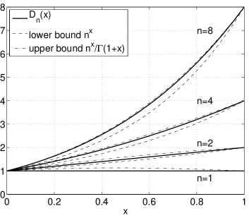
Figure 1: Diversity polynomial $D_{n}(x)$, lower bound $n^{x}$, and upper bound $n^{x}/\Gamma(1+x)$ for $n=1,2,4,8$.

III-A Main result

Theorem 1

The probability that the SIR at all antennas exceeds $\theta$ is

$$P_{n}(\theta)=\exp(-\Delta\theta^{\delta}D_{n}(\delta))\,,$$ (2)

where $D_{n}$ is the polynomial of order $n-1$ given by

$$D_{n}(x)=\frac{\Gamma(n+x)}{\Gamma(n)\Gamma(1+x)}=\frac{1}{x\beta(n,x)}\,.$$

$\beta(x,y)\triangleq\Gamma(x)\Gamma(y)/\Gamma(x+y)$ is the Beta function.

Proof:

Let $\theta_{r}=\theta r^{\alpha}$. Then the SIR condition for a single antenna is

$$\frac{hr^{-\alpha}}{I}>\theta\quad\Longleftrightarrow\quad h>\theta_{r}I\,,$$

and we have

$$P_{n}(\theta)=\mathbb{P}(h_{1}>\theta_{r}I_{1},\ldots,h_{n}>\theta_{r}I_{n})\,,$$

where $h_{i}$ are the iid fading coefficients to each antenna, and $I_{k}=\sum_{x\in\Phi}h_{x,k}\|x\|^{-\alpha}$ is the interference at each antenna, correlated through the common randomness $\Phi$. We obtain

$$P_{n}(\theta) =\mathbb{E}(e^{-\theta_{r}I_{1}}\cdots e^{-\theta_{r}I_{n}})$$

$$=\mathbb{E}\prod_{k=1}^{n}e^{-\theta_{r}I_{k}}$$

$$=\mathbb{E}\prod_{k=1}^{n}\prod_{x\in\Phi}e^{-\theta_{r}h_{x,k}\|x\|^{-\alpha}}$$

$$\stackrel{{\scriptstyle{\rm(a)}}}{{=}}\mathbb{E}\prod_{x\in\Phi}\mathbb{E}_{h}\prod_{k=1}^{n}e^{-\theta_{r}h_{x,k}\|x\|^{-\alpha}}$$

$$=\mathbb{E}\prod_{x\in\Phi}\left(\frac{1}{1+\theta_{r}\|x\|^{-\alpha}}\right)^{n}$$

$$\stackrel{{\scriptstyle{\rm(b)}}}{{=}}\exp\left(-\lambda\int_{\mathbb{R}^{2}}\left(1-\left(\frac{\|x\|^{\alpha}}{\|x\|^{\alpha}+\theta_{r}}\right)^{n}\right)\mathrm{d}x\right)\,.$$

(a) follows from the independence of the fading random variables $h_{x,i}$, and (b) follows from the probability generating functional of the PPP. The last step is the calculation of the integral, which yields the result. ∎

III-B The diversity polynomial

We term the polynomial $D$ the diversity polynomial. The first four are

$$D_{1}(x) =1$$

$$D_{2}(x) =1+x$$

$$D_{3}(x) =\tfrac{1}{2}(x+1)(x+2)$$

$$D_{4}(x) =\tfrac{1}{6}(x+1)(x+2)(x+3)\,,$$

and a general expression is

$$D_{n}(x)=\frac{1}{\Gamma(n)}\prod_{i=1}^{n-1}(i+x)=\prod_{i=1}^{n-1}\left(1+\frac{x}{i}\right)\,.$$

For all $x\in(0,1)$, since $\tfrac{\Gamma(n+x)}{\Gamma(n)}\lesssim n^{x}$,

$$n^{x}<D_{n}(x)\lesssim\frac{n^{x}}{\Gamma(1+x)}\,.$$ (3)

“$\lesssim$” indicates an upper bound with asymptotic equality, here as $n\to\infty$. The diversity polynomials for $n=1,2,4,8$ are shown in Fig. 1, together with these lower and upper bounds.

The polynomial may also be defined by its $n-1$ roots

$$D_{n}(x)=0\quad\forall x\in-[n-1]$$

and fixing either $D_{n}(0)=1$ or $D_{n}(1)=n$.

Since all the coefficients are positive, $D_{n}(x)$ is convex for $x\geq 0$ and thus bounded by

$$D_{n}(x)\leq 1+(n-1)x\,,\quad n\in\mathbb{N},\,0\leq x\leq 1\,.$$

The derivative is asymptotically

$$D_{n}^{\prime}(x)\triangleq\frac{\mathrm{d}D_{n}(x)}{\mathrm{d}x}=\Theta(n^{x}\log n)\,,\quad 0\leq x\leq 1,\,n\to\infty\,.$$ (4)

For $x=0$ and $x=1$, the result is exact, i.e., $D^{\prime}_{n}(x)\sim n^{x}\log n$, $x\in\{0,1\}$. From the bounds in (3) it follows that

$$\exp(-\Delta\theta^{\delta}n^{\delta})>P_{n}(\theta)>\exp\left(-\Delta\theta^{\delta}\frac{n^{\delta}}{\Gamma(1+\delta)}\right)\,.$$ (5)

$P_{n}(1)$ and the bounds are shown in Fig. 2.

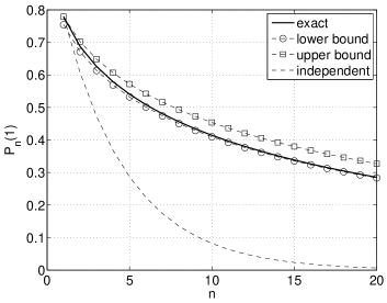
Figure 2: $P_{n}(1)$ as a function of $n$ for $\Delta=1/4$ and $\delta=1/2$, together with bounds (5), and the same probability under the assumption of independent interference.

III-C Diversity loss

If the interference was independent across the antennas, we would have

$$\tilde{P}_{n}(\theta)=\exp(-\Delta\theta^{\delta}n)\,.$$

Due to the dependence, $D_{n}(\delta)<n$ for all $\delta<1$ and only $D_{n}(1)=n$, but $\delta=1$ corresponds to $\alpha=2$, which would imply $\Delta=\infty$ and $P_{1}(\theta)=0$. The dependence increases as $\delta\downarrow 0$ (with growing $\alpha$). For $\delta=0$, $P_{n}(\theta)=P_{1}(\theta)$, $\forall n\in\mathbb{N}$ (complete correlation).

Corollary 1

The diversity loss, defined as $L(n)\triangleq\log\tilde{P}_{n}/\log P_{n}$, is

$$L(n)=n\delta\beta(n,\delta)=\frac{\Gamma(n+1)\Gamma(\delta+1)}{\Gamma(n+\delta)}\,.$$

As $n\to\infty$, $L(n)\to\infty$.

Proof:

From Thm. 1 we obtain $\log\tilde{P}_{n}/\log P_{n}=n/D_{n}(\delta)$. For the limit, we need to show that

$$\lim_{n\to\infty}\frac{D_{n}(\delta)}{n}=0\quad\text{ for }0\leq\delta<1\,.$$

This holds since

$$\frac{\Gamma(n+\delta)}{\Gamma(n+1)}\sim n^{\delta-1}\,,\quad n\to\infty\,,$$

and $\delta<1$. ∎

The fact that $D_{n}(\delta)/n\to 0$ is also apparent from the asymptotic behavior of the derivative (4).

Next we determine the conditional probability that $S_{k+1}$ holds given that $S_{1},\ldots,S_{k}$ hold.

Corollary 2

$$\mathbb{P}\left(S_{k+1}\mid S_{1}\cap\ldots\cap S_{k}\right)=\exp(-\Delta\theta^{\delta}D_{k}(\delta)\delta/k)\,,$$

and

$$\lim_{k\to\infty}\mathbb{P}\left(S_{k+1}\mid S_{1}\cap\ldots\cap S_{k}\right)=1\,.$$ (6)

Proof:

The conditional probability is $P_{k+1}/P_{k}$, which, using the recursion $D_{n+1}(x)=D_{n}(x)(1+x/n)$, yields the result. The limit (6) follows from the proof of Cor. 1. ∎

So the correlation is strong enough that, assuming $n=\infty$, for each $\epsilon>0$, there is an $m$ such that for any $k>m$, $S_{k}$ occurs with probability exceeding $1-\epsilon$ if $S_{1},\ldots,S_{m}$ hold.

III-D Correlation coefficients

Let $A_{k}=\mathbf{1}\{S_{k}\}$ be the indicator that $S_{k}$ occurs. Pearson’s correlation coefficient between $A_{i}$ and $A_{j}$, $i\neq j$, is

$$\zeta(A_{i},A_{j})=\frac{e^{-\Delta\theta^{\delta}\delta}\left(1-e^{-\Delta\theta^{\delta}(1-\delta)}\right)}{1-e^{-\Delta\theta^{\delta}}}\,,\quad i\neq j\,.$$ (7)

The correlation coefficients for different parameters are shown in Fig. 3. It is easily seen that $\zeta(A_{i},A_{j})=1$ (full correlation) for $\delta=0$, while $\zeta(A_{i},A_{j})=0$ for $\delta=1$. So a larger path loss exponent $\alpha=2/\delta$ results in higher correlation. This can be explained as follows: For large $\alpha$, the interference is dominated by a few nearby interferers, and if one of them is close enough to cause an outage at one antenna, it is likely to do so also at another. Conversely, as $\alpha\downarrow 2$, the interference is dominated by the many far interferers, each one with an independently fading channel to each antenna, which decorrelates the events.

In the high-reliability regime, where $\Delta$ or $\theta$ is small, the correlation is the largest; it is upper bounded by and approaches $1-\delta$ as $\Delta\to 0$ or $\theta\to 0$.

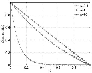
Figure 3: Correlation coefficient $\zeta$ per (7) of the indicators of the events $S_{k}$ as a function of $\delta$ for $\theta=1$ and $\Delta=0.1,\,1,\,10$. For small $\Delta$ or $\theta$, $\zeta\approx 1-\delta$.

III-E Effect on selection combining

In a selection combining scheme, a transmission is successful if $\max_{k\in[n]}\{\mathrm{SIR}_{k}\}>\theta$. The probability $p_{n}(\theta)$ that the SIR at at least one antenna exceeds the threshold follows from (2) as

$$p_{n}(\theta)\triangleq\mathbb{P}\left(\bigcup_{k=1}^{n}S_{k}\right)=\sum_{k=1}^{n}(-1)^{k+1}\binom{n}{k}P_{k}(\theta)\,.$$ (8)

Assuming independent interference, the probability of the same event would be

$$\tilde{p}_{n}(\theta)=1-\left(1-e^{-\Delta\theta^{\delta}}\right)^{n}\,,$$

which differs substantially from (8). The gap between the outage probabilities $1-p_{n}(1)$ and $1-\tilde{p}_{n}(1)$ is illustrated in Fig. 4. While there is always a gain in increasing the number of antennas $n$, it is significantly smaller than under the assumption of independent interference. Also, it can be observed that the outage probability is no longer monotonically decreasing in $\alpha$ for all $n$.

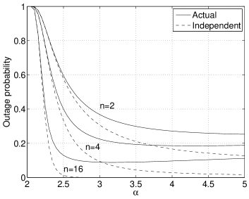
Figure 4: Outage in SIMO system with selection combining and $2$, $4$, and $16$ receive antennas for $\theta=1$ and $\Delta=\Gamma(1+\delta)\Gamma(1-\delta)/3$, where $\delta=2/\alpha$, as a function of the path loss exponent $\alpha$. The solid lines show the actual outage probability, while the dashed ones show the outage if there was no correlation in the interference.

While $\tilde{p}_{n}(\theta)\to 1$ quickly as $n\to\infty$, the asymptotic behavior of $p_{n}(\theta)$ is less clear. A plot is shown in Fig. 5. We have the following result.

Theorem 2

For all $\Delta,\theta\geq 0$, $\delta\in(0,1)$,

$$\lim_{n\to\infty}p_{n}(\theta)=1$$

and, as $n\to\infty$,

$$1-p_{n}(\theta)=\Omega(n^{-1-\epsilon})\,,\quad\forall\epsilon>0\,.$$ (9)

Proof:

Conditioned on $\Phi$, the success probability goes to $1$ since all events $S_{k}$ are independent (and have positive probability), i.e., $\lim_{n\to\infty}p_{n}(\theta\mid\Phi)=1$. Thus

$$\mathbb{E}\big{(}\lim_{n\to\infty}p_{n}(\theta\mid\Phi)\big{)}=1\,,$$

which is the same as the desired limit $\lim_{n\to\infty}\mathbb{E}(p_{n}(\theta\mid\Phi))$ by monotone convergence. For the bound on the tail probability, let $N(\theta)=\min\{k\colon\mathrm{SIR}_{k}>\theta\}$ for $n=\infty$. We have

$$\mathbb{E}N(\theta) =\sum_{k=0}^{\infty}\mathbb{P}(N(\theta)>k)$$

$$=\sum_{k=0}^{\infty}1-p_{k}(\theta)\,.$$ (10)

Replacing spatial diversity with temporal diversity, we can apply [5, Lemma 2] and set the transmit probability to $1$ (since in our case all interferers always transmit), and it follows that $\mathbb{E}N(\theta)=\infty$. So (10) diverges, which means that $1-p_{k}(\theta)$ decays more slowly than $n^{-1-\epsilon}$ for any $\epsilon>0$. ∎

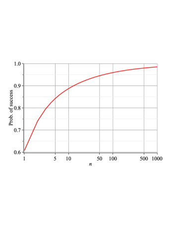
Figure 5: Success probability for selection combining as a function of the number of antennas $n$ on a logarithmic scale. $\Delta\theta^{\delta}=1/2$, $\delta=1/2$.

III-F The general two-antenna case

Corollary 3

The complete joint SIR distribution for $n=2$ is

$$\bar{P}_{2}(\theta_{1},\theta_{2}) \triangleq\mathbb{P}(\mathrm{SIR}_{1}<\theta_{1},\,\mathrm{SIR}_{2}<\theta_{2})$$

$$=1-\exp(-\Delta\theta_{1}^{\delta})-\exp(-\Delta\theta_{2}^{\delta})+$$

$$\qquad\exp\left(-\Delta\frac{\theta_{1}^{1+\delta}-\theta_{2}^{1+\delta}}{\theta_{1}-\theta_{2}}\right)\,.$$

Proof:

From Thm. 1, we obtain

$$P_{2}(\theta_{1},\theta_{2}) \triangleq\mathbb{P}(\mathrm{SIR}_{1}>\theta_{1},\mathrm{SIR}_{2}>\theta_{2})$$

$$=\exp\left(-\Delta\frac{\theta_{1}^{1+\delta}-\theta_{2}^{1+\delta}}{\theta_{1}-\theta_{2}}\right)\,$$ (11)

by the replacement

$$\left(\frac{1}{1+\theta_{r}\|x\|^{-\alpha}}\right)^{2}\;\rightarrow\;\left(\frac{1}{1+\theta_{r,1}\|x\|^{-\alpha}}\right)\left(\frac{1}{1+\theta_{r,2}\|x\|^{-\alpha}}\right)$$

in the last two lines of the derivation in the proof. Since

$$\bar{P}_{2}(\theta_{1},\theta_{2}) \triangleq\mathbb{P}(\mathrm{SIR}_{1}<\theta_{1},\,\mathrm{SIR}_{2}<\theta_{2})$$

$$=1-\mathbb{P}(\{\mathrm{SIR}_{1}>\theta_{1}\}\cup\{\mathrm{SIR}_{2}>\theta_{2}\})\,,$$

the result follows from (11). ∎

For comparison, if interference was independent, the probability (11) would be $\tilde{P}_{2}(\theta_{1},\theta_{2})=\exp(-\Delta(\theta_{1}^{\delta}+\theta_{2}^{\delta}))$.

IV Conclusions

We have derived the first results of the effect of interference correlation in Poisson networks with multi-antenna receivers. The diversity loss can be quantified exactly using the diversity polynomial. Its effects are that $\log P_{n}\propto n^{\delta}$ as opposed to $\log\tilde{P}_{n}\propto n$ for independent interference, and that the success probability in a selection combining scheme approaches $1$ at best polynomially instead of exponentially.

The larger the path loss exponent (the smaller $\delta$), the more drastic the effect of the interference correlation. Pearson’s correlation coefficient between the events that the SIR at two different antennas exceeds $\theta$ is approximately $1-\delta$ in the low-outage regime.

The results have important implications on the performance of multi-antenna networks and raise interesting questions about how to best cope with interference correlation.

References

• [1] C.-N. Chuah, D.Β N.Β C. Tse, J.Β M. Kahn, and R.Β A. Valenzuela, β€œCapacity Scaling in MIMO Wireless Systems Under Correlated Fading,” IEEE Transactions on Information Theory, vol.Β 48, pp.Β 637–650, Mar. 2002.
• [2] R.Β K. Ganti and M.Β Haenggi, β€œSpatial and Temporal Correlation of the Interference in ALOHA Ad Hoc Networks,” IEEE Communications Letters, vol.Β 13, pp.Β 631–633, Sept. 2009.
• [3] F.Β Baccelli and B.Β Blaszczyszyn, Stochastic Geometry and Wireless Networks. Foundations and Trends in Networking, NOW, 2009.
• [4] F.Β Baccelli and B.Β Blaszczyszyn, β€œA New Phase Transition for Local Delays in MANETs,” in IEEE INFOCOM’10, (San Diego, CA), Mar. 2010.
• [5] M.Β Haenggi, β€œThe Local Delay in Poisson Networks,” IEEE Transactions on Information Theory, 2011. Submitted. Available at http://www.nd.edu/~mhaenggi/pubs/tit12.pdf.
• [6] M.Β Haenggi and R.Β K. Ganti, β€œInterference in Large Wireless Networks,” Foundations and Trends in Networking, vol.Β 3, no.Β 2, pp.Β 127–248, 2008.