X-ray properties of radio-selected star forming galaxies
in the Chandra-COSMOS survey

X-ray surveys contain sizable numbers of star forming galaxies, beyond the AGN which usually make the majority of detections. Many methods to separate the two populations are used in the literature, based on X-ray and multiwavelength properties. We aim at a detailed test of the classification schemes and to study the X-ray properties of the resulting samples.

We build on a sample of galaxies selected at 1.4 GHz in the VLA-COSMOS survey, classified by Smolčić et al. (2008) according to their optical colours and observed with Chandra. A similarly selected control sample of AGN is also used for comparison. We review some X-ray based classification criteria and check how they affect the sample composition. The efficiency of the classification scheme devised by Smolčić et al. (2008) is such that $\sim 30\%$ of composite/misclassified objects are expected because of the higher X-ray brightness of AGN with respect to galaxies. The latter fraction is actually $50\%$ in the X-ray detected sources, while it is expected to be much lower among X-ray undetected sources. Indeed, the analysis of the stacked spectrum of undetected sources shows, consistently, strongly different properties between the AGN and galaxy samples. X-ray based selection criteria are then used to refine both samples.

The radio/X-ray luminosity correlation for star forming galaxies is found to hold with the same X-ray/radio ratio valid for nearby galaxies. Some evolution of the ratio may be possible for sources at high redshift or high luminosity, tough it is likely explained by a bias arising from the radio selection. Finally, we discuss the X-ray number counts of star forming galaxies from the VLA- and C-COSMOS surveys according to different selection criteria, and compare them to the similar determination from the Chandra Deep Fields. The classification scheme proposed here may find application in future works and surveys.

1 Introduction

Radio and far-infrared observations have been widely accepted as unbiased estimators of star formation (SF) in spiral galaxies for decades (see the Condon, 1992; Kennicutt, 1998, reviews). The X-ray domain has also been recognized as a SF tracer in non-active galaxies (hereafter just “galaxies”) thanks to a number of works highlighting the presence of X-ray vs. radio/infrared correlations (David et al. 1992; Grimm et al. 2003; Ranalli et al. 2003, hereafter RCS03; Gilfanov et al. 2004a). Strong absorption (i.e. with column densities $\gtrsim 10^{22}$ cm^-2) is also rare among galaxies, making the X-ray domain scarcely sensitive to extinction. Thus, an X-ray based Star Formation Rate (SFR) indicator can be considered not biased by absorption (RCS03). An interpretation framework, whose main idea is the dominance of High-Mass X-ray Binaries among the contributors to the X-ray luminosity of galaxies, has also been developed (Gilfanov et al., 2004b; Persic & Rephaeli, 2007) and is currently the subject of further investigation. The observations of deep fields, especially with Chandra, have prompted the search for galaxies at high redshifts (Alexander et al., 2002; Bauer et al., 2002; Hornschemeier et al., 2003; Ranalli, 2003). The galaxies X-ray luminosity function and its evolution has been investigated both in the local universe and at high redshift (Georgantopoulos et al. 1999; Norman et al. 2004; Georgantopoulos et al. 2005; Ranalli et al. 2005, hereafter RCS05; Georgakakis et al. 2007; Ptak et al. 2007; Lehmer et al. 2008) with also the goals of obtaining an absorption-free estimate of the cosmic star formation history, and deriving the contribution by galaxies to the X-ray background.

However, any work involving galaxies in X-ray surveys has to deal with the fundamental fact that AGN are preferentially selected in flux-limited X-ray surveys. A careful and efficient classification of the detected objects is necessary to identify the galaxies among the dominant AGN population. In early studies (Maccacaro et al., 1988) AGN were found to populate a well defined region of the X-ray/optical vs. X-ray flux plane, bounded by an X-ray/optical flux ratio $X/O=-1$ (see definition in Sect. 4.2). This threshold has been often adopted as an approximate line dividing AGN and X-ray emitting galaxies. A more robust separation between AGN and star forming galaxies is obtained (Xue et al., 2011; Vattakunnel et al., 2012) by considering several different criteria (X-ray hardness ratio, X-ray luminosity, optical spectroscopy, X-ray/infrared or X-ray/radio flux ratios). An analysis of the relative merits of the different criteria when taken separately, and of the most effective trade-offs to identify star-forming galaxies is one of the aims of this paper.

A similar need of a careful object classification has arisen in deep radio observations. It has been known since long that a population of faint radio sources associated with faint blue galaxies was emerging at radio fluxes below $\sim 1$ mJy (Windhorst et al., 1985; Fomalont et al., 1991; Richards et al., 1998; Richards, 2000). In recent years, it has been shown that a sizable fraction (about 50%) of this sub-mJy population is actually made up of AGN (Gruppioni et al., 1999; Ciliegi et al., 2003; Seymour et al., 2008; Smolčić et al., 2008; Padovani et al., 2009; Strazzullo et al., 2010). This means that an accurate screening is needed also for radio-selected faint galaxies.

This screening has been the subject of the work by Smolčić et al. (2008, hereafter S08), who made use of the extensive data sets of the COSMOS survey to analyze $\sim 2400$ sub-mJy radio sources and classified them according to a newly developed, photometry-based method to separate SF galaxies and AGN. Their method is based on optical rest-frame synthetic colours, which are the result of a principal component analysis of many combinations of narrow-band colours, and which correlate with the position of the objects in the classical BPT diagram (Baldwin et al. 1981; see Sect. 2 for details).

Here we build on this work, and use the S08 samples as the starting point for our classification of the X-ray galaxies in COSMOS. We intend to test the X-ray based selection criteria against the S08 method, and eventually refine the selection.

The Cosmological Evolution Survey (COSMOS) is an all-wavelength survey, from radio to X-ray, designed to probe the formation and evolution of astronomical objects as a function of cosmic time and large scale structure environment in a field of 2 deg² area (Scoville et al., 2007). In this paper, we build mainly on the radio (VLA-COSMOS, Schinnerer et al. 2007), X-ray (Chandra-COSMOS, or C-COSMOS, Elvis et al. 2009), and optical spectroscopic (Z-COSMOS, Lilly et al. 2007) observations. The radio data were taken at 1.4 GHz and have a RMS noise 7–10 $\mu$Jy (with the faintest sources discussed in this paper having fluxes around 60$\mu$Jy), while the X-ray data have a flux limit of $1.9\cdot 10^{-16}$ erg s^-1 cm^-2 in the 0.5-—2 keV band. The area considered here is that covered by Chandra, which is a fraction (0.9 deg²) of the whole COSMOS field. The XMM-Newton observations (XMM-COSMOS, Cappelluti et al. 2009) covered the whole field but with a brighter flux limit ($1.7\cdot 10^{-15}$ erg s^-1 cm^-2 in the 0.5–2 keV band). We focus on C-COSMOS here because its combination of area and limiting flux offers the best trade off for the subject of our study.

The structure of this paper is as follows. In Sect. 2 we define a sample of galaxies based on radio and optical selection, and subsequent X-ray detection. An AGN sample is selected with the same method to allow for comparisons. In Sect. 3 we characterize the sample, in terms of magnitudes, redshifts, and optical spectra. In Sect. 4 we review some commonly used X-ray-based indicators of star formation vs. AGN activity, and test them on our sample of galaxies; on this basis, a refined sample is then defined. In Sect. 5 we investigate the average properties of galaxies with the same radio-optical selection but without a detection by Chandra. In Sect. 6 we discuss the number of composite and mis-classified sources. In Sect. 7 we consider if the COSMOS data can further constrain the radio/X-ray correlation. Sect. 7 is devoted to an analysis of the X-ray number counts of the radio-selected COSMOS galaxies. Finally, in Sect. 9 we review our conclusions.

The cosmological parameters assumed in this paper are $H_{0}=70$ km s Mpc^-1, $\Omega_{\Lambda}=0.7$ and $\Omega_{\mathrm{M}}=0.3$.

2 Selection criteria

The catalogue of the COSMOS radio sources was published in Schinnerer et al. (2007); the objects in this catalogue were then classified by S08, on the basis of their photometry-based method. Only objects with redshift $\leq 1.2$ were considered by S08, because the errors on the classification would be larger beyond this threshold. AGN can be broadly divided in two classes: objects where the AGN dominates the entire Spectral Energy Distribution (SED), i.e. mainly QSO, and objects where it does not, such as type-II QSO, low luminosity AGN (Seyfert and LINER galaxies), and absorption-line AGN.

The fraction of type-I QSO in the VLA-COSMOS catalogue is small ($\sim 5\%$). They have higher X-ray luminosities than the SF and the other kinds of AGN, making the few type-I objects easier to separate from other classes of objects; since we are mainly interested in the properties of galaxies, we will not discuss them further. Hereafter with the term “AGN” we will only refer to the other kind of AGN (type-II and low-luminosity). These AGN have broad-band properties similar to those of SF galaxies. The main tools to disentangle SF galaxies and low-luminosity AGN are spectroscopic diagnostic diagrams (BPT diagrams Baldwin et al., 1981; Veilleux & Osterbrock, 1987; Kewley et al., 2001), which rely on the [O III 5007]/H$\beta$ and [N II 6584]/H$\alpha$ line ratios. Their main drawback is, however, the long telescope time needed to obtain good-quality spectra. Alternative methods which only build on photometric data can therefore be useful.

Based on the observation of a tight correlation between rest-frame colours of emission-line galaxies and their position in the BPT diagram, Smolčić et al. (2006) used the Sloan Digital Sky Survey (SDSS) photometry (a modified Strömgren system) to i) calculate rest-frame colours, and ii) use the Principal Component Analysis (PCA) technique to identify, among all linear combinations of colours, those which correlate best with the position in the BPT diagram. One of these combinations, named $P1$, was found to correlate strong enough with the emission line properties of SF galaxies and AGN, to be used alone for the classification.

By applying this method to the COSMOS multi-band photometric data, S08 produced a list of 340 ‘star forming’ (hereafter SF) and 601 type II/dusty/low luminosity AGN candidates. The Chandra field, which is smaller than the radio-surveyed area, contains 242 SF and 398 AGN. Some mis-classifications are inherent in any colour- or line-based methods, and a fraction of objects may also exhibit composite or intermediate properties. Thus, S08 estimate that SF samples actually may contain $\sim 20\%$ of AGN and $\sim 10\%$ of composite objects. Conversely, AGN samples contain $\sim 5\%$ SF and $\sim 15\%$ composite.

We matched the radio positions of the SF and AGN sources with those of the C-COSMOS catalogue (Elvis et al., 2009; Puccetti et al., 2009). In Fig. 1 we show the number of matched SF sources for different matching radii: the number of matches rises steeply from $0.1\arcsec$ to $0.5\arcsec$, and flattens for larger radii. To adopt a threshold for the maximum separation between the radio and X-ray coordinates, we considered that in the C-COSMOS survey some areas have been observed by Chandra only at large off-axis angles. For these areas, the point spread function (PSF) is much broader than the on-axis value ($0.5\arcsec$ FWHM), and this can also introduce errors in the determination of the source position. The position errors reported in the C-COSMOS catalogue are in fact larger than $1\arcsec$ for 221 sources out of 1761. Thus we considered all matches within $3\arcsec$, and visually inspected every match to check that the X-ray PSFs and the errors on the X-ray positions were wide enough to justify the larger threshold. Following this criterion, one match was excluded because the PSF in that position was much narrower than the distance between the radio and X-ray positions.

Figure 1: Number of matched sources in cross-correlating the C-COSMOS catalogue (Elvis et al., 2009) with the S08 sample of radio-selected star forming galaxies.

The samples of radio selected, optically classified, X-ray detected sources consist thus of 33 SF ($\sim 14\%$ of the SF-classified radio sources) and 82 AGN-type objects ($\sim 21\%$ of the AGN-classified radio sources). The breakdown of the sources according to their detection in the 0.5–2 keV, 2–7 keV and 0.5–7 keV bands is shown in Table 1. Note the presence of 10 SF candidates lacking a detection in the soft band: this hints for the presence of AGN-type objects in the SF sample, which will be discussed in detail in the next sections.

Band	SF	AGN
F+S+H	10	46
F+S	11	16
F+H	10	18
F	—	1
S	2	1
H	—	—

Table 1: Number of X-ray detected radio sources, according to their optical classification and X-ray band of detection (F: full, 0.5–7 keV; S: soft, 0.5–2 keV; H: hard, 2-7 keV).

3 Optical and radio properties

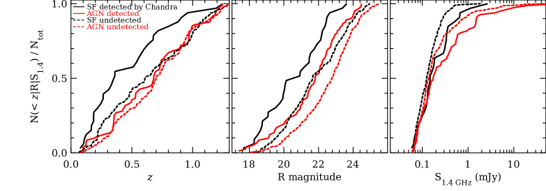
Figure 2: Relative cumulative distributions of redshift, R magnitude and radio flux in the Chandra-detected and undetected, SF and AGN galaxies subsamples.

The samples of X-ray detected vs. undetected sources exhibit different properties, as shown both in the following tests and in the cumulative distributions in Fig. 2. For the SF sample we find that:

• detected sources have brighter (observer-frame) R magnitudes than undetected ones, at a confidence level of 99.96% (according to a Wilcoxon-Mann-Whitney test; the median magnitudes are $R=20.53$ and 21.66 for the detected and undetected, respectively);

• detected sources have brighter radio fluxes than undetected, at a confidence level of 98.5% (median fluxes: ${S_{1.4\mathrm{G}Hz}}=0.148$ and 0.124 mJy, respectively);

• detected sources have lower redshifts than undetected, at a confidence level of 99.8% (median redshifts: $z=0.36$ and 0.61, respectively);

• detected sources have lower radio luminosities than undetected, at a confidence level of 97.8% (median luminosities: $S=8.7\cdot 10^{29}$ and $5.0\cdot 10^{30}$ erg s^-1 Hz^-1, respectively).

This is in line with the expectation of the detected sources being closer to us, and the undetected ones probing a larger volume where more luminous yet less common objects can be found.

The X-ray detected AGN sources also have brighter R magnitudes and radio fluxes than the undetected ones, but do not show any significant difference in the redshift distribution. The behaviour of the radio luminosity is reversed: the undetected AGN have lower radio luminosities than the detected ones.

Optical spectra of X-ray detected sources

Optical spectra are available for most of the sources with an X-ray detection from several spectroscopic campaigns: the ZCOSMOS project (Lilly et al., 2007, 2009), Magellan/IMACS surveys, the Sloan Digital Sky Survey (SDSS), (Trump et al., 2007, 2009) and deeper observations with Keck/DEIMOS and VIMOS/VLT. A simple classification based on diagnostic diagrams (Bongiorno et al., 2010), further checked by visual inspection, has been used to the determine the optical classifications (Civano & et al., 2012). Since the signal/noise ratio varies a lot in the sample, some objects have noisy spectra which can only be classified tentatively.

In the SF sample, 21 objects (out of 33) are classified as emission line galaxies; 9 are classified as AGN, and 3 have no spectral information or have spectra with low signal/noise ratios.

In the AGN sample, 25 objects (out of 82) are classified as AGN; 30 as emission line galaxies; 7 as absorption line galaxies, and 20 have no spectral information or spectra with low signal/noise ratio.

This partial overlap in the optical classification between the two catalogues is expected (see also Sect. 2), because i) the two phenomena of accretion and star formation are often present together in the same object, ii) the overlap of the areas covered by different populations (SF and AGN) in the diagnostic diagrams used by S08, iii) low-luminosity, narrow-line AGN and actively star forming galaxies can be difficult to distinguish in noisy spectra. The last point is particularly true at $z\gtrsim 0.4$, where the H$\alpha$ line is not sampled by optical spectra and, therefore, the standard BPT diagram ([O III]/H$\beta$ vs. [H II]/H$\alpha$; Baldwin et al. 1981) cannot be used in the optical spectral classification. A comparison of the observed fraction of mis-classifications and composite objects with the expectations will be presented in Sect. 6.

In the following Section, we will try and characterize further the two samples on the basis of the X-ray properties of the sources, with the aim of improving the classification.

4 X-ray characterization of the selected sources

X-ray spectra of SF galaxies are rather complex, as they include emission from hot gas, supernova remnants (thermal spectra) and X-ray binaries (non-thermal, power-law spectrum), with the thermal components being usually softer than the non-thermal ones. A detailed description of the expected spectra of the different components may be found in Persic & Rephaeli (2002). The relative importance of the spectral components may vary; however, in most cases the average flux ratio between the 0.5–2.0 keV and the 2.0–10 keV bands is the same that would be obtained if the spectrum was a power-law spectrum with spectral index $\Gamma=2.1$ and negligible absorption (RCS03; Lehmer et al. 2008). This does not imply the lack of X-ray absorption of X-rays in SF galaxies: M82 and NGC3256 are notable examples (RCS03; Ranalli et al. 2008). However, the spectral analysis of 23 SF galaxies in RCS03 did not find heavy absorption to be a general property of that sample.

The fluxes of candidate SF objects used in this paper have been recomputed from the counts by assuming the $\Gamma=2.1$ spectrum, instead of the $\Gamma=1.4$ used in Elvis et al. (2009). Conversely, for AGN we have used the latter, harder spectrum. In the following, we review a few common indicators of SF vs. AGN activity, and apply them to the SF sample for further screening.

4.1 Hardness ratio

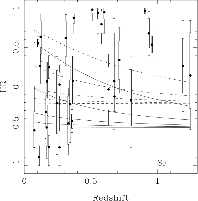
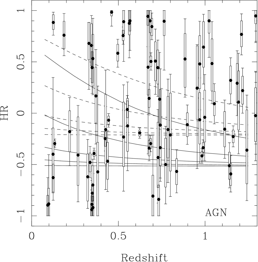
Figure 3: Hardness ratios for the SF (left) and AGN (right) X-ray detected sources. The data points, boxes and whiskers show the median and the 68% and 90% credible intervals for the HR, respectively. The superimposed lines show the HR referring to model spectra: absorbed power-laws with two different slopes ($\Gamma=2.1$, solid lines, and $\Gamma=1.4$, dotted lines) and five column densities ($N_{\rm H}=10^{20}$, $10^{21}$, $10^{21.5}$, $10^{22}$ and $10^{22.5}$ cm^-2 from bottom to top).

The hardness ratio (HR) is a simple measure of the spectral shape, defined as $HR=(H-S)/(H+S)$, where $H$ and $S$ are the net (i.e. background-subtracted) counts in the hard and soft bands respectively. It is most useful when the sources are too faint for a proper spectral analysis. The error on the HR is usually calculated by taking the uncertainties on source and background counts according to the Gehrels (1986) approximation, and applying the error propagation for Gaussian distributions. However, it has been shown that for faint sources this approach largely overestimates the errors on the HR (Park et al., 2006). To obtain a more realistic estimate of the HR uncertainties, we use the Bayesian approach described in Park et al. (2006). The source and local background counts have been extracted from the Chandra event files in soft (0.5–2 keV) and hard (2–7 keV) observer-frame energy bands. For the sources in the SF and AGN samples we show in Fig. 3 the median value of the HR posterior distributions, and the 68% and 90% highest probability density (HPD) intervals of the posterior distributions, vs. the redshifts. The HR corresponding to eight model spectra (absorbed power-laws) are also superimposed.These model HR have been calculated with XSPEC, using average effective areas (see Sect. 5) and assuming no background.

About half of the SF sources detected in C-COSMOS have a HR which is consistent with very flat or absorbed spectra ($N_{\rm H}\gtrsim 10^{21.5}$ cm^-2, or equivalently $\Gamma\lesssim 1.2$ without absorption). Conversely, about half of the AGN sources have a HR consistent with spectra steeper or less absorbed than the above thresholds.

The average hardness ratio of galaxies is the one given by a non-absorbed $\Gamma=2.1$ spectrum (RCS03). Harder spectra are sometimes indeed found in galaxies (e.g., see the slopes for single power-law fits in Dahlem et al. 1998) where they can result from bright X-ray binaries (Persic & Rephaeli, 2002). However, Swartz et al. (2004) found that the average slopes of X-ray binaries in nearby galaxies are $\Gamma=1.88\pm 0.06$ ($1.97\pm 0.11$) for binaries with luminosity larger (smaller) than $10^{39}$ erg s^-1, respectively. Only 7% (8%) of the binaries studied by Swartz et al. (2004) have slopes $\Gamma\leq 1.4$.

The large number of hard objects in the SF sample is probably due to a selection effect. Because of the C-COSMOS flux limit, the Chandra-detected SF sample only contains the brightest 14% of all the SF objects in the field of view. In addition, 30% of the S08 SF sources are expected to be composite or misclassified, as is inherent in any selection method based on diagnostic diagrams. Since AGN are on average brighter than galaxies, the composite/misclassified objects should mingle with the brightest galaxies, hence with the Chandra-detected sample rather than with the Chandra-undetected one.

4.2 X-ray/optical flux ratio

A fast and widely used, yet coarse method to classify X-ray objects is to look at their X-ray/optical flux ratio $X/O$, defined as

$$X/O=\mbox{Log}\left(F_{\rm X}\right)+0.4R+5.71$$ (1)

where $F_{\rm X}$ is the 0.5–2 keV flux, and $R$ is the optical apparent magnitude in the R filter. On average, AGN have higher $X/O$ values than SF galaxies. Given the intrinsic dispersion in the $X/O$ values for both AGN and SF galaxies, no single $X/O$ value can be used to unambiguously separate AGN from SF galaxies. However, it has been shown (Schmidt et al., 1998; Bauer et al., 2004; Alexander et al., 2002) that the value $X/O=-1$ can be taken as a rough boundary between objects powered by star formation ($X/O<-1$) and by nuclear activity ($X/O>-1$). In the SF sample, 22 objects have $X/O<-1$ (2/3 of the total sample), while 11 have $X/O>-1$. Out of this latter 11 objects, which this criterion would classify as AGN, 10 have a HR whose 68% HPD interval is consistent with a column density $N_{\rm H}\gtrsim 10^{21.5}$ cm^-2.

For comparison, the AGN sample has only 1/3 of the objects with $X/O<-1$ (27 objects out of 82).

4.3 X-ray luminosity

An X-ray luminosity of $10^{42}$ erg/s is also often used as another rough boundary between SF galaxies and AGN, with the band in which the luminosity is measured varying among different authors. While this criterion is, on its own, so unrefined that it ignores the existence of low luminosity AGN, it may still be of use when considered along with other criteria. In the SF sample, 17 objects have a 2–10 keV luminosity greater than this limit. However, it is expected that the X-ray luminosity of SF galaxies evolves with the redshift; RCS05 found that a pure luminosity evolution of the form $L_{\rm X}\propto(1+z)^{2.7}$ is a good description of the available data (see also Norman et al., 2004). Thus one should consider as AGN candidates only the objects with $L_{\rm X}>10^{42}(1+z)^{2.7}$ erg s^-1: 12 objects in the SF sample satisfy this criterion. All these 12 objects have a HR compatible with a column density larger than $10^{21.5}$ cm^-2.

4.4 Off-nuclear sources

If the X-ray position is not coincident with the galaxy centre, but is still within the area covered by the galaxy in the optical band, then the X-ray emission is probably due to an off-nuclear X-ray binary. Thus any contribution from nuclear accretion is unlikely to be significant. An off-nuclear flag is present in the catalogue of optical identifications (Civano & et al. 2012; see also Mainieri et al. 2010). The only SF source classified as off-nuclear is CXOC J100058.6+021139. No source from the AGN sample is classified as off-nuclear. While in principle this is an important selection criterion, in practice it applies to only one object in our samples, and therefore we will not consider it any further.

4.5 Classification and catalogue of sources

From the considerations made above, it seems that only about half of the objects in the SF sample have properties compatible with SF-powered X-ray emission. This hints to the presence of several objects in the sample which show intermediate, rather than SF or AGN properties. Some refinement of the S08 SF selection criteria seems thus possible by inspecting the X-ray properties of the sources.

We consider the following conditions as indicators of SF origin of the X-ray luminosity:

• $L_{2-10}\leq 10^{42}(1+z)^{2.7}$ erg s^-1, where $L_{2-10}$ is the hard X-ray (2.0-10 keV) luminosity;

• HR lower (softer) than what expected for an absorbed power-law with $\Gamma=1.4$ and $N_{\mathrm{H}}=10^{22}$ cm^-2;

• $X/O\leq-1$;

• classification as galaxy from optical spectroscopy.

For the purposes of classification, we only consider optical spectra with clear AGN-like emission line ratios as non-matching. This avoids that low signal/noise spectra can influence the classification.

Among many possibilities to combine to above criteria, we use the following method: the number of matched criteria is counted, and an object is classified accordingly. An object is assigned to class 1, if it fulfils all the conditions; to class 2, if it fulfils all conditions but one; to class 3, if there are at least two conditions not satisfied. Objects for which one condition can not be checked (e.g., a missing optical spectrum), are classified as if that condition had been matched. The idea is that an object status is affected only by conditions which have been checked and not matched.

Thus we recognize two samples of SF galaxies: one more conservative (class 1 objects), and another less conservative (objects in classes 1 or 2). Class 3 objects probably do not have the majority of their X-ray emission powered by star formation related processes. There are 8 class-1 objects; 8 class-2; and 17 class-3 objects in the SF sample.

If the same selection is applied to the AGN sample, we find 14 class-1; 6 class-2; and 62 class-3.

The classifications for both the SF and AGN sample are reported in Tables LABEL:tab:cat and LABEL:tab:catAGN, along with the other parameters of interest: X-ray fluxes, luminosities, medians of the HR posterior probability distributions, $X/O$ ratios, X-ray/radio ratios (see Sect. 7), classification from optical spectroscopy.

5 Average properties of undetected objects

Table 4: Average properties of radio-selected SF-candidates without an X-ray detection in C-COSMOS. Radio fluxes in mJy; X-ray fluxes in $10^{-18}$ erg s^-1 cm^-2; X-ray luminosities (rest frame) in $10^{40}$ erg s^-1. The counts are reported with their 68.3% error intervals. The fluxes have been calculated by fitting the stacked spectra with an imposed $\Gamma=2.1$ (this slope has the characteristic of making the 0.5–2 and 2–10 keV fluxes approximately the same; considering the rounding of non-significant digits, this explains why the fluxes are the same in the two bands). All values for the soft band are relative to the 0.5–2 keV interval, while for the hard band counts are in the 2–7 keV, and fluxes and luminosities are in the 2–10 keV bands. The allowed spectral slope ($\Gamma$) range is given in the last column.

Selection	No. of	Avg. radio	Avg.	Band	Exposure	Net	X-ray	Lumi-	$1-p_{\rm detect}$	$1-p_{\rm cts}$	$\Gamma$
	candidates	flux (mJy)	redshift		(Ms)	counts	Flux	nosity
${S_{1.4\mathrm{G}Hz}}\leq 0.20$	156	0.113	0.67	soft	16.9	$176\pm 20$	4.8	0.94	$99.99\%$	$99.99\%$	[1.5–
”	”	”	”	hard	17.7	$105\pm 25$	4.8	0.94	$99.98\%$	$>99.99\%$	2.5]
$0.20<{S_{1.4\mathrm{G}Hz}}\leq 0.63\!\!\!\!\!\!\!\!$	43	0.292	0.58	soft	4.3	$80\pm 11$	8.2	1.1	$99.96\%$	$99.92\%$	[1.7–
”	”	”	”	hard	4.5	$16^{+4.7}_{-10}$	8.2	1.1	—	—	3.8]

The method of stacking analysis allows to determine the average properties of objects which are not individually detected; it can be briefly described as follows. Candidate objects for stacking are selected from the list of SF sources in S08 which are not detected in C-COSMOS, with the additional criterion that no detected C-COSMOS source should be present within 7 arcsec from the position of the candidate. The reason is to avoid contamination from X-ray brighter sources. This does not introduce any bias in the selection of sources, because very few sources are excluded in this way (only 6 out of 209).

Because of the radio–X-ray correlation, it is expected that the average X-ray properties are dominated by the brightest radio sources. Thus it may be advisable to include in the stack only sources with a narrow spread in their radio flux, to avoid biases due to the brightest sources. We split the sample on the basis of the radio flux, dividing the candidates in two lists as follows:

1. 156 SF sources with ${S_{1.4\mathrm{G}Hz}}\leq 0.20$mJy;

2. 43 SF sources with $0.20<{S_{1.4\mathrm{G}Hz}}\leq 0.63$ mJy.

Each sub-sample is 0.5 dex wide in flux; one starts from the lowest radio flux, while the other one follows continuously.

For each list of candidates, postage-stamp size images measuring $20\times 20$ pixels (each one $0.491\arcsec$ wide) around the position of every candidate, are extracted and summed; the latter sum is hereafter called “stacked image”. If most candidates contribute some X-ray photons, then a “stacked source” appears on top of the background in the centre of the stacked image (similar results can be obtained using the software described in Miyaji et al. 2008). The wavdetect tool is then used to determine the net counts of the stacked source. This analysis was done for both the 0.5–2.0 keV and 2.0–7.0 keV bands.

The stacked source was successfully detected by wavdetect for the low-radio flux sub-sample in both bands, and for the high-radio flux in the soft band only. This is in line with the expectation that a lower number of counts should be present in the high- than in the low-radio-flux subsample: given the average fluxes and the number of positions (Table 4), $\sim 40\%$ more counts are expected in the latter than in the former.

The significance of the detection of a stacked source is best estimated with simulations: we draw as many random positions as the number of sources in the list, reproducing the same spatial distribution of the VLA-COSMOS sources, and build a stacked image from these positions. Total counts ($c_{\rm sim}$) within a radius of 3.5″ from the centre are extracted; the wavdetect software is run on the stacked image; this cycle is repeated 10000 times for each sub-sample and each band. We then define the following $p$-values:

• $p_{\rm detect}$ as the fraction of times that the wavdetect software finds a source within 1.1 arcsec of the centre of the stacked image;

• $p_{\rm cts}$ as the fraction of times that $c_{\rm sim}\geq c_{\rm stack}$, where $c_{\rm stack}$ are the total counts of the ‘real’ stacked source.

We identify the $p$-values as two estimates of the probability that the stacked source was actually a background fluctuation. The $p$-values are shown in Table 4 (actually, $1-p$ is shown, i.e. the probability that the source is not a fluctuation).

Using the source and background regions defined above, and a power-law average spectrum with $\Gamma=2.1$, we extracted the net counts and derived the fluxes and luminosities shown in Table 4.

Stacked X-ray spectra have also been extracted for the two subsamples, using CIAO 4.0. Background spectra have been extracted around the source positions, by taking 4 circular background regions for each source, each background region having the same radius of the source region, and being placed $10\arcsec$ east, north, west, or south of the source. This ensures that the background is the most accurate, given the actual sky positions of the sources. Then, we removed background positions which fell within $7\arcsec$ from any Chandra-detected source. Response matrices have been calculated considering the stacked source like it was an extended source consisting of many small pieces scattered around the detector area, weighted by the photons actually present in each position.

Figure 4: Confidence contours for relevant parameters of simple models of stacked spectra of SF sources and (for comparison) AGN sources not detected by Chandra (sources with radio flux $F<0.20$ mJy).The contours are shown at levels of $\Delta\mathrm{C}$: +2.92, +5.63, +8.34 above minima. Solid lines: SF sources; dotted lines: AGN.

The stacked spectra were fitted with a model which is the weighted sum of many absorbed power-laws; the number of power-law components is the number of sources in the stack. Each absorbed power-law is redshifted to the $z$ of the corresponding source. The slope and absorption are free parameters, but are assumed to be the same for all sources. The weights are proportional to the radio fluxes. Finally, observer-frame absorption due to the Galaxy is added. This method allows to fully account for the redshift distribution of the sources. We used XSPEC version 11.3.2 for this analysis.

The confidence contours for the parameters are shown in Fig. 4 (solid curves) for the bin with sources with ${S_{1.4\mathrm{G}Hz}}\leq 0.2$ mJy. The spectrum is consistent with moderately steep photon indices ($1.5\lesssim\Gamma\lesssim 2.5$). This behaviour is expected for star forming galaxies (see Sect. 4). The bin with sources with $0.2<{S_{1.4\mathrm{G}Hz}}\leq 0.63$ mJy (not shown) has a lower number of X-ray photons in the spectrum and thus a wider range of slopes allowed, yet the spectrum is still consistent with the other bin.

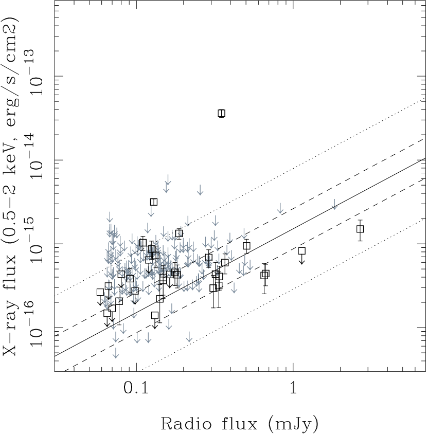
Figure 5: Radio vs. X-ray (0.5–2 keV) fluxes for the VLA-COSMOS SF sources detected in C-COSMOS. Detected sources are marked with squares and error bars. The black squares with an attached arrow mark the sources which are not detected in the band to which the panel refers, but are detected in any other of the C-COSMOS bands. Conversely, the grey upper limits show the sources without a detection in any X-ray band, hence without an entry in the C-COSMOS catalogue. The solid line shows the RCS03 relationship, K-corrected to the average redshift of the detected sources ($z=0.46$), while the dashed lines show the 1$\times$ and 3$\times$ standard deviation of the relationship.

For comparison, in Fig. 4 (dotted curves) we show also the confidence contours for stacked spectra of 207 AGN, selected from the S08 sample in the same radio flux intervals of the SF galaxies, and also not detected by Chandra. The average redshifts of these AGN are not significantly different from the SF ones. The AGN X-ray spectra are flatter; this is probably the result of absorption and of redshift (summing absorbed spectra of sources at different redshift leads to flat or inverted spectra, like in the case of the cosmic X-ray background). While a single power-law model is probably simplistic, a more detailed modeling would be beyond the scope of this paper. The average X-ray fluxes for the AGN, calculated with the best-fit slopes, are $7.2\cdot 10^{-18}$ ($4.8\cdot 10^{-17}$) erg s^-1 cm^-2 for the bin with ${S_{1.4\mathrm{G}Hz}}\leq 0.2$ mJy and $3.0\cdot 10^{-18}$ ($1.0\cdot 10^{-17}$) erg s^-1 cm^-2 for the bin with $0.2<{S_{1.4\mathrm{G}Hz}}\leq 0.63$ mJy in the 0.5–2 (2–10) keV band. The allowed ranges for the AGN spectral slopes are [0.4–0.9] and [0.6–2.2] for the ${S_{1.4\mathrm{G}Hz}}\leq 0.2$ mJy and $0.2<{S_{1.4\mathrm{G}Hz}}\leq 0.63$ mJy bins, respectively.

6 Mis-classified and composite objects

The fractions of X-ray detected objects whose classification based on optical spectral line ratios (where available) is different from that based on the synthetic $P1$ colour in S08 are $9/33\sim 27\%$ (SF sample) and $37/82\sim 45\%$ (AGN sample). These numbers are of the same magnitude of those quoted in Sects. 4.1,4.2, 4.3, though it is important to stress that different criteria yield different mis-classified and composite (hereafter MCC) objects.

These fractions should be compared with the number of class 3 objects in the SF sample ($17/33\sim 51\%$) and of classes 1-2 in the AGN sample ($20/82\sim 24\%$).

However, these fractions do not take into account the large number of X-ray undetected objects and should probably be considered as upper limits to the true fractions of MCC objects. In fact, the stark difference found between the average X-ray spectra of undetected SF and AGN sources (Sect.5) would rather suggest much lower fractions of MCC. A lower limit to the true fractions of MCC can be derived by assuming that the MCC are only present among the X-ray detected sources. In this case, the fractions would be $17/242\sim 7\%$ ($20/398\sim 5\%$) for the class 3 (classes 1-2) in the SF (AGN) sample. The rationale for this assumption would be, for the SF sample, that galaxies with an AGN contribution are on average brighter in X-rays than the galaxies without and thus are more likely to be X-ray detected. For the AGN sample, it would be that intense star formation could cause X-ray emission at a level similar to that of a low-luminosity or absorbed active nucleus.

The fractions reported by S08 (30% of MCC in the SF and 20% in the AGN sample; see Sect. 2) are intermediate between our upper and lower limits’ estimates, and therefore we regard them as in agreement with our findings. In the following, we use the method described in Sect. 4.5 to identify the MCC candidates. The same method cannot be applied to X-ray undetected objects, and therefore the optical colour-based classification is used for them in the remaining of this paper.

7 The X-ray/radio flux ratio

Correlations between X-ray and radio luminosities of star forming galaxies, and between the X-ray and far infrared (FIR) ones, are well established for the local universe and have been tested for objects up to $z\sim 1$ (Bauer et al. 2002; RCS03; Gilfanov et al. 2004a; Persic & Rephaeli 2007). Both the radio and FIR luminosity are tracers of the star formation rate (SFR). These correlations are linear, and imply that in absence of any contribution from an AGN, the X-ray emission is powered by star-formation related processes. High-Mass X-ray Binaries (HMXB) seem to have the same luminosity function in all galaxies, only normalised according to the actual SFR. Thus, if HMXB are the dominant contributors to the X-ray emission, the X-ray luminosity is a tracer of the SFR (Grimm et al., 2003; Gilfanov et al., 2004b; Persic & Rephaeli, 2007). The other possibly dominant contributors to the X-ray emission are the Low-Mass X-ray Binaries (LMXB), whose number scales with the galaxy stellar mass. The actual balance of the two populations thus depends on the ratio between SFR and mass, thus it is possible that there is some evolution of the correlation due to the mass build-up by the galaxies with the cosmic time.

The VLA- and C-COSMOS surveys contain a sizable number of objects at medium-deep redshifts on which the correlation might be tested. However, many objects have radio fluxes close to the VLA-COSMOS flux limit. This is clearly visible in Fig. 5, where we show the radio and X-ray fluxes and upper limits for all the SF galaxies in the C-COSMOS field. Since we account for the X-ray upper-limits, the main source of potential bias is the radio flux limit; the results may therefore be biased towards radio-brighter-than-X-rays objects. To partially mitigate this effect, we split the sample in two redshift bins, defined as follows.

The knee of the radio LF of galaxies is found at a luminosity $L_{\mathrm{k}}\sim 1.5\cdot 10^{29}$ erg s^-1 Hz^-1 at 1.4 GHz (see, e.g., Fig.2 in RCS05). We define the first bin as the redshift interval in which all objects with luminosity $\geq\frac{1}{2}L_{\mathrm{k}}$ can be observed. This corresponds to $z\leq 0.2$. In other words, this redshift threshold guarantees that the luminosities around $L_{\mathrm{k}}$ are included in the sampled volume. While this bin does not contain a strictly volume-limited subsample, here the selection bias should be mitigated as much as possible, and still the bin includes a sizable number of objects.

The second bin contains the remaining objects, i.e. those with $z>0.2$. Finally, we refer to calculations made on all objects as a third bin named “any-$z$”.

For most of the objects, the 0.5–2 keV flux limit is a few times larger than what expected from the radio flux limits and the radio/X-ray correlation. Many objects therefore only have X-ray upper limits, which need to be properly accounted for. The 2–10 keV limit is about one order of magnitude larger and thus this band is not considered in this Section.

The hypothesis we would like to test is if the COSMOS data are consistent with the extrapolation of the RCS03 correlation, or if they require substantially different parameters. This kind of question is usually what Bayesian methods are most suited to answer. The ratio

$$q=\mbox{Log}(F_{0.5-2\mathrm{keV}}/{S_{1.4\mathrm{G}Hz}})$$ (2)

may be defined in the same way of the analogous $q$ parameter often employed in testing the radio/FIR correlation of spiral galaxies (Condon, 1992). Non-detections in X-rays therefore lead to upper limits for the $q$’s and can be properly accounted for.

To include the K-correction in the $q$’s, we consider the individual redshifts of the sources and assume average power-law spectra with average slopes. Using X-rays (0.5–2.0 keV luminosity less than $10^{42}$ erg s^-1) to remove bright AGN from the VLA-CDFS survey (Kellermann et al., 2008; Tozzi et al., 2009), a radio spectral energy index $\alpha\sim 0.69$ can be assumed for the galaxies.

The radio/X-ray correlation is described by its slope (here assumed unity), its mean $\bar{q}$, and its standard deviation $\sigma$. The two latter parameters are the subject of the present statistical analysis, and need prior probability distributions, which we take as follows:

• $\bar{q}_{\mathrm{prior}}$ is assumed to follow a normal distribution with mean $\bar{q}_{0}$ and standard deviation $\sigma_{0}$ taken equal to the values found by RCS03 in the local universe ($\bar{q}_{0}=11.10$ and $\sigma_{0}=0.24$);

• the standard deviation $\sigma_{\mathrm{prior}}$ is assumed to be uniformly distributed.

In Fig. 6, the prior distribution is represented as the grey shade.

Figure 6: Credible contours for the logarithmic X-ray/radio ratio $q$. The Bayes formula was used to derive the posterior probability for $q$, shown as contours (levels relative to 50%, 68.3% and 90%). The blue continuous and the green long-dashed contours refer to SF objects with $z\leq 0.2$ and $z>0.2$, respectively. The red short-dashed contours refer to SF objects at any redshift (i.e., the sum of the two bins). The green long-dashed arrow shows the correction that should be made to $q$ for the $z>0.2$ and any-$z$ bins to account for the bias due to radio selection. The grey-scale background shows the prior (a darker grey means a higher probability density). The yellow asterisk shows the $q_{0}$ value from RCS03.

The Bayesian posterior probabilities were calculated with the Montecarlo method (Meeker & Escobar, 1998); the credible contours for the mean and standard deviations of $q$ are also shown in Fig. 6, along with the RCS03 estimate.

The posterior distribution for $q$ and $\sigma$ is consistent with the RCS03 values, within the 68.3% HPD area for the $z\leq 0.2$ and any-$z$ bins, and within the 90% Highest Posterior Density (HPD) area for the $z>0.2$ bin. However, the centres of the posterior distributions of the $z>0.2$ and the any-$z$ bins appear to be shifted to lower values of $q$.

The $z>0.2$ and the any-$z$ bins allow a larger $\sigma$ than RCS03 (by a factor $\lesssim 2$), while the $z\leq 0.2$ bin also allows smaller $\sigma$. The reasons for the larger dispersion may include the large number of upper limits, uncertainties on the K-correction, and a residual contamination by AGN of the objects with X-ray upper limits.

One possible explanation of a smaller $q$ at high redshift is that the radio luminosity is evolving in redshift at a faster pace than the X-ray one. The possibilities for an increased efficiency of the radio emission might include different details of cosmic ray acceleration and propagation, or larger magnetic fields at high redshift. However, it has been shown that magnetic fields of a strength similar to those found in local galaxies are in place at $z\sim 1$ (Bernet et al., 2008).

The two redshift bins can also be seen, approximately, as two luminosity bins. Thus, a different interpretation may be that $q$ is luminosity dependent, as suggested by Symeonidis et al. (2011) that the X-ray/far-infrared ratio may be lower in UltraLuminous InfraRed Galaxies (ULIRGs) than in normal galaxies with lower luminosities. If the analysis presented in this Section is repeated by dividing the sample in two luminosity bins (radio luminosities lower and higher than $4\cdot 10^{29}$ erg s^-1 Hz^-1, which is the median luminosity of the SF sample), then a picture quite similar to Fig. 6 is obtained: the high-luminosity bin favours a smaller $q$ than the low-luminosity bin, yet there is a sizable fraction of the parameter space which is allowed by both bins, and which contains the RCS03 value.

However, the redshift bins whose data prompt for the evolution only sample the high-luminosity tail of the radio luminosity function, and it is possible that a selection bias is part of the explanation: it may be that radio-luminous objects have lower X-ray luminosity than average. In fact, it has been shown (Vattakunnel et al., 2012) that galaxies in the Chandra Deep Fields, whose average X-ray luminosity is about one order of magnitude lower than those presented here, follow the same X-ray/radio correlation of galaxies in the local universe.

An estimate of the bias due to the radio selection may be done with the method employed by Sargent et al. (2010) for the infrared/radio correlation (see also Kellermann 1964; Condon 1984; Francis 1993; Lauer et al. 2007), in which the bias for a flux limited survey (where the luminosity function of the sources is not fully sampled) depends only on the scatter of the correlation $\sigma$ and on the slope of the differential number counts $\beta$:

$$\Delta q_{\mathrm{b}ias}=\mathrm{ln}(10)\,(\beta-1)\,\sigma^{2}\sim 0.18$$ (3)

where $\beta\sim 2.35$ (see Sect. 7) and $\sigma$=0.24. The amount of correction is shown in Fig. 6 as the green dashed arrow. Applying this correction to the $z>0.2$ and any-$z$ bins would mostly remove the redshift (or luminosity) evolution of $q$. This correction needs not to be applied to the $z\leq 0.2$ bin because here the luminosity function should be almost correctly sampled. However, this correction should be only taken as a first-order approximation, because one of its hypotheses is that the scatter of the X-ray/radio correlation is described by a Gaussian function. Because the $\Delta q_{\mathrm{b}ias}$ is sensitive to the shape of wings of the function, any deviation of the correlation from a Gaussian would require Eq. (3) to be modified accordingly (Lauer et al., 2007).

For these reasons, a further investigation of this issue with deeper observations in both the radio and X-ray bands, and including a proper statistical treatment of truncated data could be an interesting subject for a follow-up analysis.

8 Demographics of star forming galaxies

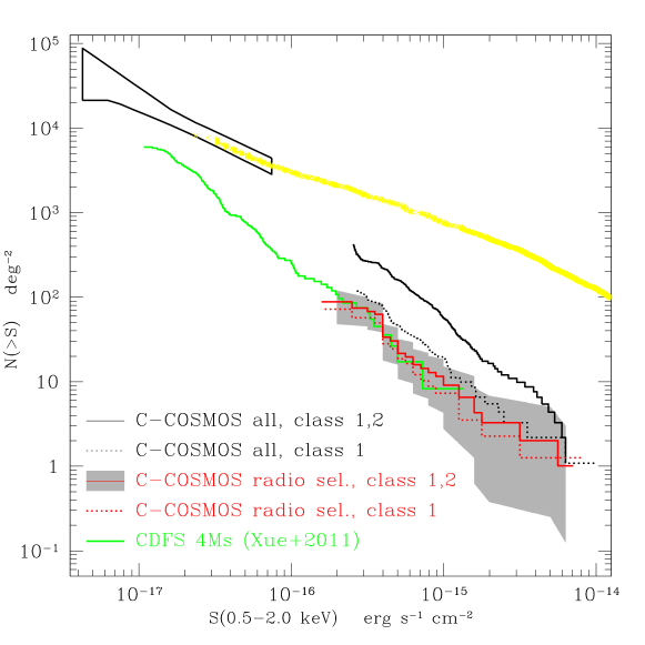
Figure 7: Number counts of SF sources detected in the VLA- and C-COSMOS surveys, compared to the CDFS determinations.
Dotted red histogram: VLA+C-COSMOS class-1 SF candidates. Solid red histogram, with grey error area: VLA+C-COSMOS class-1,2 SF candidates. Dotted black histogram: C-COSMOS class-1 SF candidates (not requiring radio detection). Solid black histogram: C-COSMOS class-1,2 SF candidates (not requiring radio detection). Green histogram: galaxy candidates in the CDFS (Xue et al., 2011); their selection criteria are similar to ours for the dotted red histogram. The thick yellow line and the horn-shaped symbol refer to the total (AGN+SF) number counts and fluctuations in the Chandra Deep Fields (Moretti et al., 2003; Miyaji & Griffiths, 2002a, b).

An important test for the selection criteria described so far is to check for the size of the population of candidate SF X-ray galaxies. In this Section, we describe four different alternatives, which are plotted in Fig. 7. The galaxy X-ray number counts from the Chandra Deep Fields (CDFS Xue et al., 2011) are also shown for reference.

First, we consider the 22 class 1 objects from Tables LABEL:tab:cat and LABEL:tab:catAGN. This is the strictest selection that we discuss, since it requires that an object is radio-detected, and that all the X-ray based criteria are fulfilled. It should thus be considered as a lower limit. We keep the assumption that a criterion is considered fulfilled if the relevant data are lacking, as done in Sect. 4.5. The number counts for this selection are plotted in Fig. 7 as the dotted red histogram.

The addition of the 14 class 2 objects to the above selection gives the solid red histogram, with the errors shown as the grey area. We only plot the errors for this selection, in order not to clutter the figure; however, they can be taken as representative of the other alternatives. The ratio between the class-1-only and the class$\leq 2$ histograms is about a factor of 2 at high X-ray fluxes and less than that at lower fluxes.

A different approach is to discard the radio selection criterion, and to apply the X-ray based criteria to the whole C-COSMOS catalogue(Elvis et al., 2009; Civano & et al., 2012). This opens the possibility to include a larger number of composite SF/AGN and of low luminosity AGN in the selection. A number of 63 class-1 and 192 class-2 objects are selected in this way. The dotted and solid black histograms show the result for the class-1 and class$\leq 2$ objects, respectively. While the class-1 histogram lies a factor of $\sim 2$-3 above the red ones and is still within the 1–2$\sigma$ errors for the above determinations, a much larger difference (a factor of $\sim 7$) is observed for the class$\leq 2$ histogram.

The latter Log $N$–Log $S$ should be regarded as a likely overestimate for the X-ray galaxy number counts. In fact, if this histogram were extrapolated at fainter fluxes, it would predict a number of galaxy which, summed to expected number of AGN from synthesis models (Gilli et al., 2007; Treister et al., 2009), would be incompatible with the observed total Log $N$–Log $S$. A further hint comes from the integration of the galaxy X-ray luminosity function: the theoretical Log $N$–Log $S$ relations in RCS05 would lie on average a factor of 3 below the histogram. (The same Log $N$–Log $S$ are however consistent with the other three determinations).

The galaxy number counts were derived by Xue et al. (2011) for the 4Ms CDFS by considering the following criteria: X-ray luminosity, photon index, X/O, optical spectroscopic classification, and X-ray/radio ratio. The criteria were joined is a similar manner to what done here for the class-1 sources. It is thus not surprising that, although each threshold is somewhat different from what used in this paper, the final result is very similar to the counts of radio-selected galaxies presented here. A power-law with the form $\mbox{Log}\ N(>S)=-1.35\,\mbox{Log}\ S-19.15$ may thus be considered a useful description of both Xue et al. (2011) and our determinations of the galaxy X-ray number counts.

9 Conclusions

We have presented the X-ray properties of a sample of 242 SF galaxies in the C-COSMOS field, selected in the radio band and classified according to the optical colours with the method described in S08. This method builds on the definition of a synthetic rest-frame colour, which can be calculated from narrow-band photometry in several bands, and which has been shown to correlate with the position in the BPT diagram (Smolčić et al., 2006). It has a similar power to the BPT diagram, with the advantage of not requiring expensive spectral observations.

In Chandra observations, 33 objects were detected. A comparison sample of 398 candidate type-II AGN (with 82 detections) is also presented.

We have reviewed some X-ray based selection criteria commonly used in the literature, and analyzed how they affect the composition of the SF and AGN samples. We have thus refined the SF sample, and recovered some objects from the AGN one, on the basis of the following parameters:

• hardness ratio;

• X-ray luminosity;

• X-ray/optical flux ratio;

• classification from optical spectroscopy.

This is a small yet effective set of indicators based only on X-ray and optical properties. We also mention that a similar method has been applied by Xue et al. (2011) in the Chandra Deep Field South.

We have proposed two refined subsamples of C-COSMOS SF galaxies, based on the absence of AGN-like properties, one (class-1) being more strict in its criteria than the other (class$\leq 2$), containing 8 and 16 objects respectively. If the same method is applied to the AGN sample, 14 objects may be recovered as SF under the stricter method, and 20 under the more liberal one; these objects may be composite, or may have been misclassified by the optical colour method.

Of 33 detections in the SF sample, 17 exhibit AGN-like properties in terms of hardness ratio, non-detection in the 0.5-2.0 keV band, optical spectrum, X-ray/optical flux ratio and absolute X-ray luminosity. Among 82 detections in the AGN sample, 20 have SF-like properties. Thus the fraction of composite/misclassified objects is 50% for the SF sample and 25% for the AGN, while S08 reported fractions of 30% and 20%, respectively. The larger fractions observed here are likely to be explained as a selection effect, due to the fact that AGN are on average brighter than galaxies in the X-rays.

Conversely, the stacked spectra of X-ray undetected SF and AGN are significantly different: the SF one can be fit with power-law spectra with $1.5\lesssim\Gamma\lesssim 2.5$, while the AGN one is flatter ($0.4\lesssim\Gamma\lesssim 0.9$). This suggests that the two samples do have different physical properties and that the fractions of composite/misclassified are actually lower for X-ray-undetected objects. Thus we regard the fraction of mis-classified and/or composite objects to be in line with the expectations from S08.

We have investigated if the radio/X-ray luminosities correlation (RCS03) applies to our data, and if there is any evidence for redshift evolution of the correlation parameters. A subsample of SF objects at $z\leq 0.2$ yields an X-ray/radio ratio fully consistent with the local RCS03 estimate. Data at larger redshifts are still consistent with the local value. Some evolution towards lower X-ray/radio ratios is possible, but at least part of the evolution may be explained by selection biases arising in flux-limited surveys. Further analysis of deeper data, or the use of statistical techniques appropriate to truncated data may be necessary.

We have presented the number counts of the C-COSMOS SF galaxies according to different selection criteria, and compared them to the number counts of the CDFS galaxies (Xue et al., 2011). Considering only the radio-selected class-1, or the radio-selected class$\leq 2$, or dropping the radio selection and only considering class-1, all lead to estimates which are consistent to each other within the 1–2$\sigma$ errors. Dropping the radio selection and considering class$\leq 2$ objects gives an overestimate of the galaxy number counts.

Further observations of the COSMOS field with Chandra would allow a much better determination of the X-ray demographics of the SF galaxies at the redshifts probed in this paper. By extending the coverage to the full 2 deg², with a uniform exposure of 180 ks over 1.7deg² (the HST-observed area), the final size of the X-ray detected COSMOS SF galaxy sample should be of the order of 200.

The AEGIS survey (Nandra et al., 2005) is similar in methodology to COSMOS, and currently has an observed area and flux limit similar to C-COSMOS, and recent observations have added deeper coverage (uniform exposure of 800 ks) to a 0.6 deg² sub-field. Even deeper is the exposure (4 Ms) in the Chandra Deep Field South (CDFS) field in the GOODS survey. Though the probed area is smaller (0.2 deg²; Xue et al. 2011; Vattakunnel et al. 2012), the CDFS already provides 179 objects classified as galaxies (24% of the total). This latter field also has a 3 Ms coverage with XMM-Newton, which is providing good quality spectroscopy (Comastri et al., 2011).

The surveys described above have also extensive optical spectroscopy, and have been observed in the far infrared by Spitzer and Herschel. The inclusion of infrared data could provide a further improvement in the object classification, and together with optical photometry could allow to break down the AGN and host galaxy contributions for the composite objects.

Finally, these data sets and the classifications done insofar could be used as testbeds for innovative statistical methods in object recognition and classification. This would be especially useful in light of the future large surveys, both in X-rays (e.g., eROSITA) and in optical (LSST, Pan-STARRS, SNAP).

2

Table 5: Catalogue of radio-selected SF-candidate sources with an X-ray detection in C-COSMOS. The columns report: VLA and Chandra names, Chandra ID from Elvis et al. (2009), redshifts, X-ray fluxes (in erg s^-1 cm^-2) and luminosities (rest-frame; in erg s^-1) for the soft (0.5–2.0 keV) and hard (2.0-10 keV) bands; rest-frame hardness ratios; X-ray/optical flux ratios; X-ray/radio flux ratio $q$; classification from optical spectroscopy (A: absorption line galaxy; E: emission line galaxy; L: spectrum with low signal/noise ratio; T1: type-I AGN; T2: type-II AGN); final classification (see Sect. 4.5).

VLA name

Chandra name

Chandra

redshift

Flux

Flux

Lum.

Lum.

HR

X/O

$q$

Opt.

Class

(COSMOSVLA-)

(CXOC-)

ID

(soft)

(hard)

(soft)

(hard)

ratio

class.

J095844.86+021100.3

J095844.8+021100

327

0.633

$7.27\cdot 10^{-16}$

$2.98\cdot 10^{-15}$

$1.24\cdot 10^{42}$

$5.08\cdot 10^{42}$

-0.03

-0.78

11.74

E

3

J095903.81+020316.8

J095903.8+020317

1065

1.247

$2.20\cdot 10^{-16}$

$<2.32\cdot 10^{-15}$

$1.99\cdot 10^{42}$

$<2.09\cdot 10^{43}$

0.14

-0.83

11.19

T1

3

J095915.63+020856.6

J095915.6+020857

2800

0.168

$4.57\cdot 10^{-16}$

$<1.82\cdot 10^{-15}$

$3.60\cdot 10^{40}$

$<1.43\cdot 10^{41}$

-0.52

-2.07

11.41

T2

2

J095924.03+022708.1

J095924.0+022708

2247

0.714

$<8.24\cdot 10^{-16}$

$4.39\cdot 10^{-15}$

$<1.89\cdot 10^{42}$

$1.01\cdot 10^{43}$

0.34

$<$-0.33

$<$10.86

E

3

J095934.70+021228.9

J095934.7+021229

1542

0.345

$4.18\cdot 10^{-16}$

$<2.18\cdot 10^{-15}$

$1.68\cdot 10^{41}$

$<8.76\cdot 10^{41}$

-0.22

-1.59

10.81

E

1

J095941.06+021501.3

J095941.0+021501

1295

0.880

$<3.13\cdot 10^{-16}$

$4.53\cdot 10^{-15}$

$<1.39\cdot 10^{42}$

$2.01\cdot 10^{43}$

0.68

$<$-0.78

$<$11.67

E

3

J095945.19+023439.4

J095945.2+023439

1272

0.124

$4.34\cdot 10^{-16}$

$4.46\cdot 10^{-15}$

$1.75\cdot 10^{40}$

$1.79\cdot 10^{41}$

0.64

-2.29

11.13

L

2

J095947.61+015555.9

J095947.6+015555

811

0.27a

$4.28\cdot 10^{-16}$

$<1.71\cdot 10^{-15}$

$1.56\cdot 10^{41}$

$<6.23\cdot 10^{41}$

-0.46

-1.55

11.37

—

1

J095953.91+024043.3

J095953.9+024043

612

0.537

$<6.42\cdot 10^{-16}$

$1.35\cdot 10^{-14}$

$<3.05\cdot 10^{41}$

$6.42\cdot 10^{42}$

0.88

$<$-0.53

$<$11.73

E

3

J100002.06+020132.6

J100002.0+020132

1499

1.193

$<4.33\cdot 10^{-16}$

$3.98\cdot 10^{-15}$

$<3.50\cdot 10^{42}$

$3.22\cdot 10^{43}$

0.26

$<$-0.15

$<$11.73

E

3

J100004.53+020852.2

J100004.5+020852

1126

0.959

$8.65\cdot 10^{-16}$

$1.66\cdot 10^{-14}$

$4.08\cdot 10^{42}$

$7.83\cdot 10^{43}$

0.54

-0.43

11.84

E

3

J100005.31+020135.3

J100005.4+020134

1083

0.311

$3.96\cdot 10^{-16}$

$2.84\cdot 10^{-15}$

$1.25\cdot 10^{41}$

$8.97\cdot 10^{41}$

0.62

-1.66

11.43

E

2

J100010.15+024141.4

J100010.2+024140

623

0.221

$1.50\cdot 10^{-15}$

$7.59\cdot 10^{-15}$

$1.21\cdot 10^{41}$

$6.12\cdot 10^{41}$

0.07

-1.43

10.75

T2

2

J100011.90+021425.1

J100011.9+021425

1517

0.602

$<1.48\cdot 10^{-16}$

$3.68\cdot 10^{-15}$

$<2.23\cdot 10^{41}$

$5.55\cdot 10^{42}$

0.95

$<$-1.10

$<$11.36

T2

3

J100013.58+021230.8

J100013.5+021230

1164

0.188

$3.18\cdot 10^{-16}$

$<2.89\cdot 10^{-15}$

$1.14\cdot 10^{40}$

$<1.03\cdot 10^{41}$

0.26

-1.92

10.98

E

2

J100013.72+021221.4

J100013.7+021221

1297

0.186

$5.97\cdot 10^{-16}$

$5.40\cdot 10^{-15}$

$5.91\cdot 10^{40}$

$5.34\cdot 10^{41}$

0.25

-1.82

11.21

T2

3

J100022.94+021312.5

J100022.9+021313

1221

0.186

$6.85\cdot 10^{-16}$

$<1.15\cdot 10^{-15}$

$6.74\cdot 10^{40}$

$<1.13\cdot 10^{41}$

-0.76

-2.00

11.37

E

1

J100023.82+020105.4

J100023.8+020106

1092

0.361

$4.08\cdot 10^{-16}$

$<2.59\cdot 10^{-15}$

$1.89\cdot 10^{41}$

$<1.20\cdot 10^{42}$

0.08

-1.64

11.08

E

1

J100027.77+015704.2

J100027.7+015705

1096

0.26a

$3.83\cdot 10^{-16}$

$<1.03\cdot 10^{-15}$

$8.33\cdot 10^{40}$

$<2.24\cdot 10^{41}$

-0.77

-1.50

11.62

—

2

J100028.55+022725.9

J100028.5+022725

1535

0.248

$4.42\cdot 10^{-16}$

$<1.14\cdot 10^{-15}$

$8.22\cdot 10^{40}$

$<2.12\cdot 10^{41}$

-0.20

-1.69

10.82

E

1

J100045.10+022110.5

J100045.1+022110

962

0.265

$1.03\cdot 10^{-15}$

$4.04\cdot 10^{-15}$

$2.25\cdot 10^{41}$

$8.84\cdot 10^{41}$

0.03

-0.85

11.97

T2

3

J100051.34+021117.7

J100051.3+021117

12650

0.802

$2.06\cdot 10^{-16}$

$<1.32\cdot 10^{-15}$

$6.24\cdot 10^{41}$

$<4.00\cdot 10^{42}$

-0.17

-1.16

11.42

E

1

J100054.74+021611.3

J100054.7+021611

24

0.678

$1.33\cdot 10^{-15}$

$5.23\cdot 10^{-15}$

$2.68\cdot 10^{42}$

$1.05\cdot 10^{43}$

-0.12

-0.41

11.85

E

3

J100056.16+015642.7

J100056.1+015642

366

0.360

$3.16\cdot 10^{-15}$

$6.57\cdot 10^{-15}$

$1.40\cdot 10^{42}$

$2.91\cdot 10^{42}$

-0.44

-0.72

12.39

T2

3

J100057.46+015901.6

J100057.4+015902

368

0.511

$<1.70\cdot 10^{-16}$

$6.22\cdot 10^{-15}$

$<1.73\cdot 10^{41}$

$6.34\cdot 10^{42}$

0.98

$<$-1.42

$<$11.39

T2

3

J100058.69+021139.6

J100058.6+021139

11100

0.110

$3.66\cdot 10^{-16}$

$<1.00\cdot 10^{-15}$

$1.13\cdot 10^{40}$

$<3.09\cdot 10^{40}$

-0.89

-2.21

11.39

E

1

J100059.70+015820.2

J100059.6+015820

1508

0.674

$<2.65\cdot 10^{-16}$

$1.65\cdot 10^{-15}$

$<5.25\cdot 10^{41}$

$3.27\cdot 10^{42}$

0.07

$<$-1.20

$<$11.65

E

2

J100100.67+021641.4

J100100.7+021640

3718

0.166

$9.46\cdot 10^{-16}$

$<2.00\cdot 10^{-15}$

$7.20\cdot 10^{40}$

$<1.52\cdot 10^{41}$

-0.32

-1.76

11.27

T2

2

J100101.94+014800.3

J100101.9+014800

284

0.909

$<1.40\cdot 10^{-16}$

$9.19\cdot 10^{-15}$

$<5.76\cdot 10^{41}$

$3.78\cdot 10^{43}$

0.96

$<$-1.24

$<$11.03

E

3

J100114.96+014348.4

J100114.9+014348

298

0.578

$<4.30\cdot 10^{-16}$

$1.25\cdot 10^{-14}$

$<5.93\cdot 10^{41}$

$1.72\cdot 10^{43}$

0.80

$<$-1.13

$<$11.42

E

3

J100129.41+013633.4

J100129.3+013634

1678

0.104

$3.61\cdot 10^{-14}$

$6.34\cdot 10^{-13}$

$1.00\cdot 10^{42}$

$1.76\cdot 10^{43}$

0.55

-0.62

13.01

E

3

J100129.95+021705.2

J100129.9+021705

2078

0.076

$2.96\cdot 10^{-16}$

$<1.13\cdot 10^{-15}$

$4.16\cdot 10^{39}$

$<1.59\cdot 10^{40}$

-0.55

-2.45

10.98

E

1

J100203.09+020907.1

J100203.1+020906

551

0.556

$<2.74\cdot 10^{-16}$

$6.29\cdot 10^{-15}$

$<3.40\cdot 10^{41}$

$7.81\cdot 10^{42}$

0.94

$<$-1.42

$<$11.45

E

3

3