Accurate and homogeneous abundance patterns in solar-type stars of the solar neighbourhood: a chemo-chronological analysis

Abstract

Aims. We report the derivation of abundances of C, Na, Mg, Si, Ca, Sc, Ti, V, Cr, Mn, Fe, Co, Ni, Cu, Zn, Sr, Y, Zr, Ba, Ce, Nd, and Sm in a sample of 25 solar-type stars of the solar neighbourhood, correlating the abundances with the stellar ages, kinematics, and orbital parameters.

Methods. The spectroscopic analysis, based on data of high resolution and high signal-to-noise ratio, was differential to the Sun and applied to atomic line equivalent widths supplemented by the spectral synthesis of C and ${\rm C}_{2}$ features. We also performed a statistical study by using the method of tree clustering analysis, searching for groups of stars sharing similar elemental abundance patterns. We derived the stellar parameters from various criteria, with average errors of 30 K, 0.13 dex, and 0.05 dex, respectively, for $T_{\rm eff}$, $\log{g}$, and [Fe/H]. The average error of the [X/Fe] abundance ratios is 0.06 dex. Ages were derived from theoretical HR diagrams and membership of the stars in known kinematical moving groups.

Results. We identified four stellar groups: one having, on average, over-solar abundances ($\langle$[X/H]$\rangle$ = +0.26 dex), another with under-solar abundances ($\langle$[X/H]$\rangle$ = $-$0.24 dex), and two with intermediate values ($\langle$[X/H]$\rangle$ = $-$0.06 and +0.06 dex) but with distinct chemical patterns. Stars sharing solar metallicity, age, and Galactic orbit possibly have non-solar abundance ratios, a possible effect either of chemical heterogeneity in their natal clouds or migration. A trend of [Cu/Fe] with [Ba/Fe] seems to exist, in agreement with previous claims in the literature, and maybe also of [Sm/Fe] with [Ba/Fe]. No such correlation involving C, Na, Mn, and Zn is observed. The [X/Fe] ratios of various elements show significant correlations with age. [Mg/Fe], [Sc/Fe], and [Ti/Fe] increase with age. [Mn/Fe] and [Cu/Fe] display a more complex behaviour, first increasing towards younger stars up to the solar age, and then decreasing, a result we interpret as possibly related to time-varying yields of SN Ia and the weak s-process in massive stars. The steepest negative age relation is due to [Ba/Fe], but only for stars younger than the Sun, and a similar though less significant behaviour is seen for Zr, Ce, and Nd. [Sr/Fe] and [Y/Fe] show a linearly increasing trend towards younger stars. The [Cu/Ba] and [Sm/Ba] therefore decrease for younger stars. We found that [Ba/Mg], [Ba/Zn], and [Sr,Y,Ba/Sm] increase but only for stars younger than the Sun, whereas the [Sr/Mg], [Y/Mg], [Sr/Zn], and [Y/Zn] ratios increase linearly towards younger stars over the whole age range.

1 Introduction

The Galactic chemical and dynamical history can be well framed by a series of average “laws” (see e.g. Edvardsson et al. 1993; McWilliam 1997), namely: the age-metallicity relation (which in principle is accessible by more than one chemical element), the [element/element] abundance ratios, the stellar metallicity frequency distribution, the Galactic metallicity gradient, and the star formation history, besides their mutual relationships as a function of space and time. The success of the Galactic chemical evolution models is to be judged by their ability to reproduce these constraints (see Allen & Porto de Mello 2011).

In recent years there has been growing recognition that, even though such average laws are meaningful and fundamental, there may be considerable underlying complexity in the real Galaxy that has gone at least partly unappreciated. In the present age of very large spectroscopic databases and precise abundances for numerous chemical elements, a successful model must harmonise stellar evolution inputs such as the initial mass function, the star-formation rate, and mass loss processes, connecting these to the specific properties of Galactic components, and a large diversity of spatial and temporal structures, differing timescales for stellar nucleosynthetic yields and their sensitivities to differing metallicities.

During the evolution of the Galactic disc, nucleosynthesis in successive generations of stars occurs together with dynamical interactions with the interstellar gas. The states of the Galaxy in past periods of its evolution are still preserved in the abundance distributions of solar-type stars, which constitute an ideal population to study the chemical evolution. These stars have an age dispersion comparable to the age of the Galaxy. They are similar to the Sun in many physical parameters, allowing the application of a differential analysis and the consequent minimisation of theoretical shortcomings of atmospheric models and systematic errors. In addition, their chemical composition does not change in consequence of the mixing processes in their surfaces, which means that the present abundance of a given element is the same as in the time of their formation (an exception are the abundances of Li, Be, and B, but these elements are not considered in this work). Therefore, the chemical abundance of solar-type stars, combined with kinematical, orbital, and evolutionary parameters (mass and age), provide a powerful tool to investigate the chemical and dynamical evolution of the Galaxy.

Over the last decade, several works have analysed the composition of disc dwarf stars of spectral types F and G (Chen et al. 2000; Reddy et al. 2003; Bensby et al. 2005; Chen et al. 2008; Neves et al. 2009). The metallicity ranges have become wider, the number of stars and elements studied has become larger, stars with and without detected planets have been compared, and the chemical distinction between thin and thick stellar population has been refined. Here we specifically ask, when regarded in as high a level of detail as possible with present techniques, to what extent the relative abundances of chemical elements can be traced as a function of age, the nature of underlying nucleosynthetic processes, and whether these properties can be statistically grouped for the nearby solar-type stars, defining “snapshots” relevant to the chemo-chronological evolution of the Galaxy.

In this work we present a multi-elemental spectroscopic analysis of a sample of 25 solar-type stars in the solar neighbourhood, all members of the thin disc stellar population (excepting one star in the transition between thin and thick discs). We have performed the determination of atmospheric parameters (effective temperature, metallicity, surface gravity, and micro-turbulence velocity), mass, age, kinematical and orbital parameters, and elemental abundances based on equivalent widths or spectral synthesis. Three different criteria were used to pin down the stellar effective temperatures, and they showed excellent internal consistency. We have also performed a statistical study of our abundance results using the method of tree clustering analysis (Everitt et al. 2001), through which we looked for stellar groups that share similar abundances in [X/H], where X represents one given element. Four groups were identified and then analysed in terms of their relations with [Fe/H], age, [Ba/Fe], kinematics, and Galactic orbits.

Despite the small range in metallicity, our sample stars cover a broad range in age, and possible trends with age were traced. The relation between [X/Fe] and [Ba/Fe] for a few elements has also been considered given the Ba-rich nature of some of our stars. In particular, we investigated previous correlations with Na and Cu suggested by Castro et al. (1999). Finally, considering the results of Rocha-Pinto et al. (2006) that, on average, metal-poor and old stars tend to have larger $|$$R_{\rm m}$$-R_{\odot}|$ (where $R_{\rm m}$ is the mean orbital distance from the Galactic centre), we have looked for any relations involving the stellar groups of the clustering analysis and the kinematic and orbital parameters of the sample.

Though limited in size, our sample was carefully built up to undergo an homogeneous and detailed analysis, based on spectra with high resolution and high signal-to-noise ratio, in order to achieve a precision as high as possible in our determinations. Particular care was exercised to derive the stellar atmospheric parameters from different and independent criteria, in an attempt to limit the abundance uncertainties as much as possible.

In Sect. 2 we describe the observations and the reduction process. In Sect. 3 we present the methods used to derive the atmospheric parameters and the chemical abundances. The stellar evolution, kinematics, and orbits are presented in Sect. 4. The tree clustering method is described in Sect. 5, and all the results are discussed in Sect. 6. Finally, we present our conclusions in Sect. 7.

2 Observations and data reduction

The sample stars were selected from the Bright Star (Hoffleit & Jaschek 1982) and Hipparcos (ESA 1997) catalogues according to the following conditions:

• Solar neighbourhood stars in a distance $\leq$ 40 pc;

• Stars brighter than $V$ = 6.5 and with declination $<+20\,\degr$;

• Stars with effective temperature and metallicity distributed over about $5500\leq$ $T_{\rm eff}$$\leq 6100$ K and $-0.3\leq$ [Fe/H] $\leq 0.3$ dex, respectively, which represents the colour index range $0.52\leq$ ($B-V$) $\leq 0.78$ from the ($B-V$) calibration described in Sect. 3.4 (Eq. 3); and

• Stars with no information of duplicity (capable of significantly affecting the spectroscopy) available in the astrometric and spectroscopic binary catalogues of Hoffleit & Jaschek (1982), Warren & Hoffleit (1987), Batten et al. (1989), and Duquennoy & Mayor (1991); the possibility of duplicity was afterward revised in the Washington Double Star Catalogue (Mason et al. 2001) and in the survey of Raghavan et al. (2010), and no close-in companions that could affect our analysis were found.

Based on these criteria, 99 F, G, and K dwarfs and subgiants were selected, out of which 25 stars were observed and analysed in this work. Our sample, shown in Table 1, contains F and G dwarf and subgiants stars from the thin disc stellar population, excepting the star HD 50806, which is probably in the transition between thin and thick discs.

The observations were carried out at the Cerro Tololo Inter-American Observatory (CTIO, Chile) in two different runs: $i)$ 15 stars were observed in March 25-26, 1994 using the Cassegrain échelle spectrograph mounted on the 4 m telescope, with the red camera, 140 $\mu$m slit, and Tek CCD detector of $1024\times 1024$ pixels ($24\times 24\leavevmode\nobreak\ \mu$m pixel size), and with a gain of 1 e^-/ADU; the spectra have resolution $R\sim 29\,000$ and cover the wavelength range 4370$-$6870 Å divided into 46 orders; and $ii)$ 10 stars were observed in November 8-15, 1997 using the bench-mounted échelle spectrograph and a $750\leavevmode\nobreak\$mm folded Schmidt camera attached to the 1.5 m telescope; the same CCD was used; the spectra have resolution $R\sim 46\,000$ and cover the wavelength range 4550$-$6520 Å divided into 37 orders.

Table 1: The 25 sample stars. The mean values of S/N ratios measured in continuum windows around $\lambda\lambda$ 4500$-$5000 Å are listed for the stars and for the two sunlight spectra (Ganymede).

Object	$V$		Sp. type	$\langle$ S/N $\rangle$
First run (March 26-25, 1994):
Ganymede	5	.10	G2 V	450
HD 20807	5	.24	G0 V	430
HD 43834	5	.08	G7 V	370
HD 84117	4	.93	F8 V	410
HD 102365	4	.89	G2 V	370
HD 112164	5	.89	F9 V	400
HD 114613	4	.85	G3 V	400
HD 115383	5	.19	G0 V	320
HD 115617	4	.74	G7 V	370
HD 117176	4	.97	G5 V	410
HD 128620	$-$0	.01	G2 V	450
HD 141004	4	.42	G0 V	520
HD 146233	5	.49	G2 V	420
HD 147513	5	.37	G5 V	290
HD 160691	5	.12	G3 IV-V	400
HD 188376	4	.70	G5 IV	310
Second run (November 8-15, 1997):
Ganymede	5	.10	G2 V	410
HD 1835	6	.39	G3 V	230
HD 26491	6	.37	G1 V	310
HD 33021	6	.15	G1 IV	240
HD 39587	4	.39	G0 V	510
HD 50806	6	.05	G5 V	300
HD 53705	5	.56	G0 V	370
HD 177565	6	.15	G6 V	290
HD 181321	6	.48	G2 V	220
HD 189567	6	.07	G2 V	260
HD 196761	6	.36	G8 V	400

The two subsamples, although observed in different conditions, were both selected based on the same criteria and will be treated as an homogeneous single sample. The spectra collected in the first run have, on average, signal-to-noise ratio (S/N = 395 $\pm$ 60) slightly larger than those of the second one (S/N = 320 $\pm$ 90) and, despite having smaller resolution, may provide smaller uncertainties in some parameters estimated here. Nevertheless, all spectra have S/N $>$ 200 in the blue region, which warranties spectral line profiles good enough to the equivalent width measurements. Any differences in the error estimates are discussed throughout the paper whenever needed.

Two spectra of the sunlight reflected by Ganymede were also observed, one in each run. The S/N ratios were estimated using continuum windows in the spectra selected by inspection of the solar flux atlas of Kurucz et al. (1984) (hereafter the Solar Flux Atlas) and the solar line identifications catalogue of Moore et al. (1966) (hereafter the Solar Lines Catalogue). The mean values $\langle$ S/N $\rangle$ measured in the wavelength range 4500$-$5000 Å are listed in Table 1. For larger wavelengths the S/N ratios are even higher, approaching twice that for $\lambda$4500 in the range 6000$-$6500 Å.

The spectra were reduced using IRAF routines for order identification and extraction, background subtraction (including bias and scattered light), flat-field correction, wavelength calibration, radial-velocity shift correction, and flux normalisation. The wavelength calibration was performed onto the stellar spectra themselves using lines selected by inspection of the Solar Flux Atlas and the Solar Lines Catalogue. The normalisation of the continuum is a very delicate and relevant step in the analysis procedure, since the accuracy of the equivalent width measurements is very sensitive to a faulty determination of the continuum level. Therefore, continuum windows free from telluric or photospheric lines were carefully selected also based on the Solar Flux Atlas and the Solar Lines Catalogue.

3 Spectroscopic analysis

A differential spectroscopic analysis relative to the Sun was performed to determine the atmospheric parameters and the chemical abundance of several elements in our sample. The analysis was based on the equivalent widths of atomic lines measured in the spectra, and on the spectral synthesis of carbon atomic and molecular lines. The two groups of stars (15 observed in the first and 10 in the second run) were treated in comparison with the Ganymede spectrum of their respective run.

3.1 Equivalent widths and atomic line parameters

Atomic lines of the elements Na, Mg, Si, Ca, Sc, Ti, V, Cr, Mn, Fe, Co, Ni, Cu, Zn, Sr, Y, Zr, Ba, Ce, Nd, and Sm were selected throughout the spectral range for equivalent width ($EW$) measurements. The lines were chosen based on the Solar Flux Atlas and the Solar Lines Catalogue, selecting only those for which the profiles were sufficiently clean from blends in order to provide reliable measurements. For both solar and stellar spectra, the $EW$ values of more than 7500 lines of these elements (about 300 lines per star) were measured by hand by Gaussian function fit using IRAF routines.

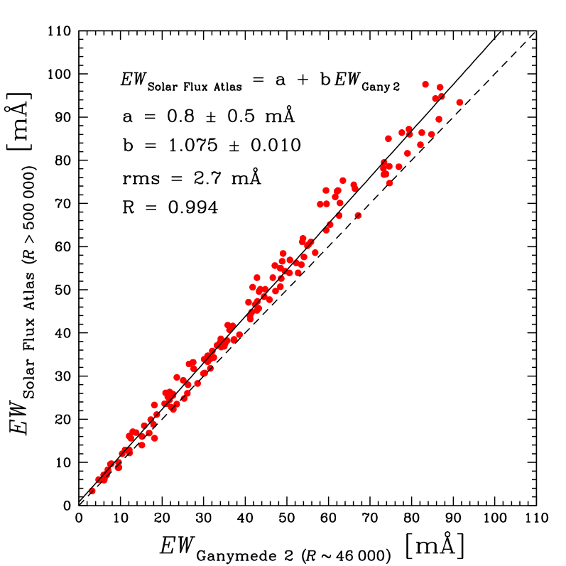
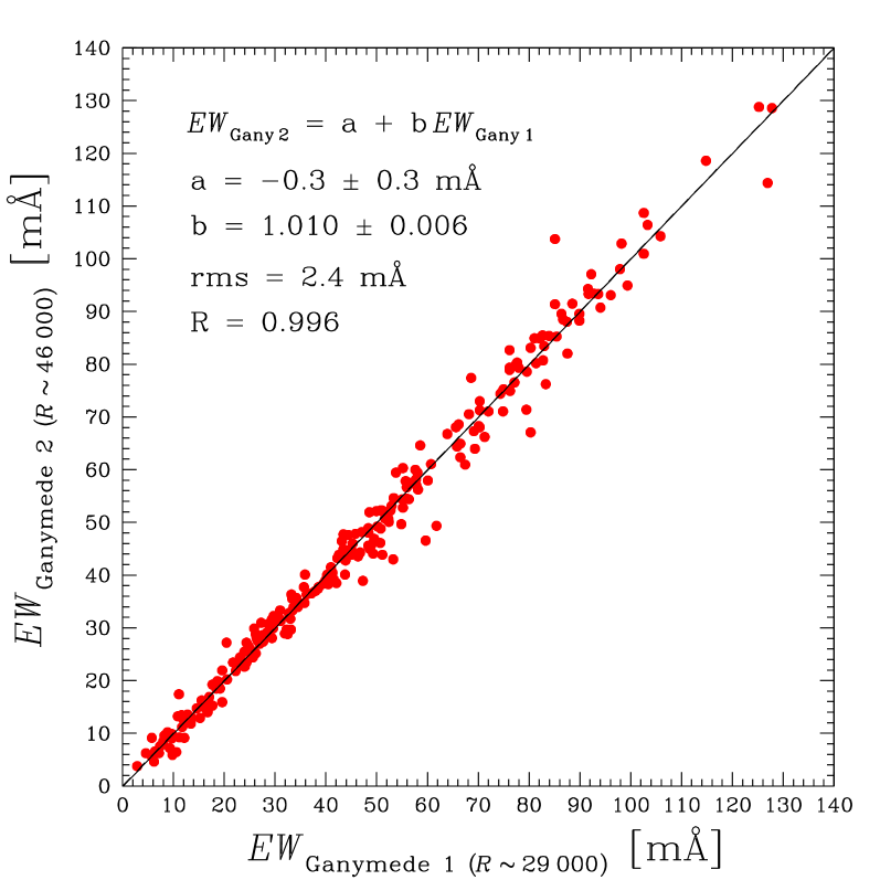
Figure 1: Left panel: comparison of the EWs measured in this work in the Ganymede spectrum (second observation run) by Gaussian function fit to those measured by Meylan et al. (1993) in the Solar Flux Atlas by Voigt function fit; filled circles represent 145 lines of several elements; the linear regression (solid line) is the same expressed by Eq. 2. Right panel: comparison of the EWs listed in Table 8 of all lines in the Ganymede spectra in common to both runs after the conversions according to Eq. 1 and 2; the coefficients of the linear regression (solid line) are shown.

Strong line profiles are better described by Voigt functions than by Gaussian functions. We show in Fig. 1 (left panel) a comparison of the $EW$s measured in this work in the Ganymede spectrum of the second observation run (Gany 2) by Gaussian function fit to those measured in the Solar Flux Atlas ($R>500\,000$ and S/N $\sim$3000) by Voigt function fit (Meylan et al. 1993). A similar diagram was obtained using the Ganymede spectrum of the first run (Gany 1) and the following relations represent the linear least square regressions fitted to both diagrams:

$$EW_{\rm Solar\,Flux\,Atlas}=(0.3\pm 0.6)+(1.065\pm 0.012)\,EW_{\rm Gany\,1}$$ (1)

$$EW_{\rm Solar\,Flux\,Atlas}=(0.8\pm 0.5)+(1.075\pm 0.010)\,EW_{\rm Gany\,2}$$ (2)

where $EW$ is given in mÅ. The standard deviations and the cross-correlation coefficients are, respectively, $\sigma$ = 3.4 mÅ and $r$ = 0.991 for Eq. 1, and $\sigma$ = 2.7 mÅ and $r$ = 0.994 for Eq. 2. Therefore, to reduce possible systematic uncertainties and provide direct comparison with other works, all our $EW$s were transformed to a common system using the regression coefficients of these equations (the constant terms have no statistical significance within 2$\sigma$). The regressions were derived in order to have a direct transformation to the Solar Flux Atlas system. We also did the converse (using $EW_{\rm Ganymede}$ vs. $EW_{\rm Solar\,Flux\,Atlas}$ diagrams) for comparison, and the resulting regressions are comparable with those of Eq. 1 and 2, within 1$\sigma$.

The wavelength and lower-level excitation potential ($\chi$) of the atomic lines used were taken from the Solar Lines Catalogue. The oscillator strengths ($gf$) were computed using a solar model atmosphere applied to the $EW$s of Ganymede (converted using Eq. 1 and 2) in order to provide the standard solar abundances of Grevesse & Noels (1993). The adopted solar abundances are of course inconsequential in a differential analysis.

The solar and stellar model atmospheres were computed with a code kindly supplied by Dr. Monique Spite (Meudon Observatory, Paris) that interpolates the model-atmosphere grid from Edvardsson et al. (1993). We used an updated version of the original code from Spite (1967). The fundamental atmospheric parameters (effective temperature $T_{\rm eff}$, metallicity [Fe/H], surface gravity $\log{g}$, and micro-turbulence velocity $\xi$) and the population ratio of helium and hydrogen atoms ($n_{\rm He}/n_{\rm H}$) are taken as input. For the Sun, the adopted parameters are $T_{\rm eff}$= 5777 K, $\log{g}$= 4.44, $\xi$ = 1.3 km s^-1, $n_{\rm He}/n_{\rm H}$ = 0.1, and $\log{\epsilon}_{\,\odot}$ = 7.50 (the solar Fe abundance).

The spectral lines used and their parameters are listed in Table 8, in which the $EW$s are the raw values (before the conversion). We do not list the $EW$s of the other stars but they are available upon request.

The atomic lines of the elements Mg, Sc, V, Mn, Co, and Cu have important hyperfine structure (HFS). Their $gf$ values, listed in Table 9, were taken from Steffen (1985) and also revised according to the $EW$s of Ganymede and the standard solar abundances of Grevesse & Noels (1993), as done for the other elements. For the elements Zn, Sr, Y, Zr, Ce, Ba, and Nd, for which theoretical HFS exist, either their effects are negligible or the spectral lines used are too weak to depend on the HFS assumption. For the elements without HFS data listed in Steffen (1985), values of neighbouring multiplets were adopted. The only exception was the Mg line at $\lambda$5785.285, for which no HSF information was available. Its $gf$ value, listed in Table 8, was obtained in the same way as those lines without HFS. This is not a strong line ($EW<60$ mÅ) so that the error induced in the Mg abundance determination is not important. del Peloso et al. (2005) have recently shown that for Mn and Co the differences in their abundances computed using different values of HFS are not greater than 0.10 dex.

The HFS of Ba, and also its isotopic splitting, are of some importance only for the line at $\lambda$6496.9, and can be neglected for the lines at $\lambda$5853.7 and $\lambda$6141.7 (see Korotin et al. 2011). However, for the 25 stars of our sample we have found a good agreement among the abundances yielded by the three lines, with a mean standard deviation of 0.07 dex. Moreover, a test performed using only $\lambda$5853.7 and $\lambda$6141.7 indicated that the global behaviour and trends found in the abundance diagrams, as well as all our conclusions involving the Ba results would not change if only these two lines were used.

Concerning the fact that we used two spectrographs with different spectral resolutions, we performed a test in which we degraded the spectrum of Ganymede and of the metal-rich star HD 1835, both observed in the second observation run, to match the resolution of the first run. New values of EWs were then obtained, and no systematic differences were found when they are compared with the original measurements. Moreover, a comparison of the EWs of Ganymede listed in Table 8 and converted according to Eq. 1 and 2 (see Fig. 1, right panel) demonstrates that the equivalent widths of the two observation runs were properly transformed to a common system, reinforcing our assumption of an homogeneous analysis.

3.2 Derivation of atmospheric parameters

In order to determine the fundamental atmospheric parameters we developed a code that iteratively calculates these parameters for a given star based on initial input values. The so called excitation effective temperature ($T_{\rm eff}^{\rm exc}$) was calculated through the excitation equilibrium of neutral iron by removing any dependence in a [Fe I/H] vs. $\chi$ diagram. The micro-turbulence velocity was obtained by removing the dependence of [Fe I/H] on $EW$, and the ionisation surface gravity ($\log{g_{\rm ion}}$) was computed through the ionisation equilibrium between Fe I and Fe II. Finally, the metallicity was yielded by the $EW$ of Fe I lines.

The temperature used in our abundance analyses was the excitation effective temperature, which is a better representation of the temperature stratification of the line forming layers. In order to compute the stellar luminosity with more reliability by also accounting for any consequence due to small LTE departures, we also considered two other temperature indicators, which are described in Sect. 3.4.

Table 2 lists the spectroscopic atmospheric parameters of the program stars. An estimate of their uncertainties was performed based on the analysis of HD 146233 and HD 26491, which are representative stars in our sample (from the first and second runs, respectively) with regard to their parameters and quality of the spectroscopic data. For both stars we have similar errors and they were obtained as follows:

Table 2: Atmospheric parameters from our spectroscopic analysis. For comparison, the evolutionary surface gravity computed as described in Sect. 4.1 (Eq. 7) is also shown.

Star	$T_{\rm eff}^{\rm exc}$ [K]	$\log{g_{\rm ion}}$	$\log{g_{\rm evol}}$	$\xi$ [km s-1]	[Fe/H]
Sun	5777	4.44	4.44	1.30	0	.00
HD 1835	5890	4.52	4.49	1.66	0	.21
HD 20807	5878	4.51	4.44	1.33	$-$0	.22
HD 26491	5820	4.38	4.28	1.38	$-$0	.09
HD 33021	5750	4.14	4.05	1.40	$-$0	.20
HD 39587	6000	4.52	4.48	1.72	0	.00
HD 43834	5630	4.47	4.44	1.23	0	.11
HD 50806	5610	4.12	4.03	1.36	0	.02
HD 53705	5810	4.32	4.26	1.34	$-$0	.22
HD 84117	6074	4.20	4.27	1.56	$-$0	.06
HD 102365	5643	4.47	4.40	1.04	$-$0	.28
HD 112164	6031	4.05	3.87	1.79	0	.32
HD 114613	5706	3.97	3.87	1.55	0	.15
HD 115383	6126	4.43	4.26	1.61	0	.23
HD 115617	5587	4.41	4.42	1.22	0	.00
HD 117176	5587	4.13	3.91	1.36	$-$0	.04
HD 128620	5857	4.44	4.31	1.45	0	.23
HD 141004	5926	4.28	4.18	1.49	0	.03
HD 146233	5817	4.45	4.42	1.32	0	.05
HD 147513	5891	4.63	4.48	1.41	0	.04
HD 160691	5777	4.32	4.19	1.40	0	.27
HD 177565	5630	4.42	4.43	1.24	0	.08
HD 181321	5810	4.34	4.56	2.30	$-$0	.06
HD 188376	5514	3.71	3.61	1.55	0	.00
HD 189567	5700	4.44	4.32	1.22	$-$0	.27
HD 196761	5410	4.44	4.49	1.08	$-$0	.32

• The uncertainty in $T_{\rm eff}^{\rm exc}$ is related to the standard error of the angular coefficient of the linear regression fitted to the [Fe I/H] vs. $\chi$ diagram. The temperature is changed until this coefficient is of the same order of its error. The difference between the best value and the previous one from the last iteration provides the uncertainty $\sigma$($T_{\rm eff}^{\rm exc}$) = 30 K;

• The uncertainty in metallicity is the standard deviation of the abundance yielded by individual Fe I lines, which is $\sigma$([Fe/H]) = 0.05 dex;

• To estimate the uncertainty in $\log{g_{\rm ion}}$, its value is changed until the difference between the averaged abundance yielded by Fe I and Fe II lines is of the order of their internal errors ($\sim$0.05 dex), which led to an uncertainty $\sigma$($\log{g_{\rm ion}}$) = 0.13 dex;

• The uncertainty in the micro-turbulence velocity is estimated regarding the [Fe I/H] vs. $EW$ diagram. The $\xi$ value is modified until the angular coefficient of the regression is of the same order of its error. An uncertainty $\sigma$($\xi$) = 0.04 km s^-1 was found for this parameter.

The spectroscopic atmospheric parameters were used to compute the model atmospheres, which in turn are required in the abundance determination. In our analysis, we used the model-atmosphere grid derived by Edvardsson et al. (1993) for stars with effective temperatures from 5250 to 6000 K, surface gravity from 2.5 to 5.0 dex, and metallicity from $-$2.3 to +0.3 dex (with small extrapolations when needed). These are 1D, plane-parallel, constant flux, line-blanketed, and LTE models computed over 45 layers.

The model atmospheres are, essentially, subject to errors in the atmospheric parameters, in the LTE simplifications, and in the thermal homogeneity assumption. However, the effects of non-LTE and thermal inhomogeneities are hopefully minor for the elements and the stellar types studied here, being more important for low metallicity and low surface gravity stars (Edvardsson et al. 1993; Asplund 2005). Possible errors induced by such simplified assumptions are dominated by other sources of uncertainties. In addition, in a differential analysis, the errors in the stellar atmospheric structure are of second order.

We also investigated what would be the effects on the derived abundances if another model-atmosphere grid were used. We compared Edvardsson and Kurucz models and, using the same equivalent widths, gf values, and atmospheric parameters obtained from a solar spectrum, we found that the differences in abundance [X/Fe] for most of the elements are of the order of 0.03 dex or smaller, achieving a maximum of 0.07 dex. We note that these values are for the Sun and represent the differences between the two sets of model atmospheres. The effects of these differences when computing the stellar abundances relative to the Sun are minimised in a differential approach.

3.3 Abundance determination and their uncertainties

The abundance of the elements studied were determined using an adapted version of a code also supplied by Dr. Monique Spite. The code takes into account the solar $gf$ values and the stellar model atmospheres (computed using the atmospheric parameters of each star) to calculate the abundances that fits the equivalent widths measured in the spectra (transformed according to the procedure described in Sect. 3.1). The results of this abundance determination are presented and discussed in Sect. 6.

Table 3: A comparison between the estimated abundance errors $\sigma_{\rm est}$ (see Sect. 3.3 and 3.5) and the dispersions of these abundances around the mean $\sigma_{\rm disp}$ for elements with N = 5 or more lines measured. For each element of each observation run the larger value was adopted to represent the errors $\sigma$([X/Fe]).

[X/Fe]	HD 146233			HD 26491
	$\sigma_{\rm est}$	$\sigma_{\rm disp}$	N	$\sigma_{\rm est}$	$\sigma_{\rm disp}$	N
C	0.07	–	2	0.07	–	2
Na	0.03	–	2	0.06	–	2
Mg	0.03	–	4	0.06	–	4
Si	0.05	0.06	11	0.06	0.03	17
Ca	0.03	0.04	6	0.05	0.05	13
Sc	0.06	0.03	6	0.09	0.03	13
Ti	0.07	0.04	24	0.10	0.04	38
V	0.07	0.07	8	0.11	0.04	11
Cr	0.06	0.04	14	0.07	0.04	29
Mn	0.04	0.05	8	0.06	0.04	11
Co	0.07	0.05	9	0.11	0.04	12
Ni	0.04	0.03	23	0.07	0.04	26
Cu	0.04	–	3	0.07	–	3
Zn	0.05	–	1	0.06	–	1
Sr	0.06	–	1	0.07	–	1
Y	0.07	0.05	5	0.09	0.05	5
Zr	0.09	–	3	0.08	–	3
Ba	0.06	–	3	0.08	–	3
Ce	0.07	0.07	5	0.12	–	3
Nd	0.16	–	2	0.12	–	2
Sm	0.09	–	1	0.15	–	1

The main sources of uncertainties in the abundance determination come from the errors in the $EW$s (the most important), the $gf$ values, the atmospheric parameters, and the adopted model atmospheres (these two latter are discussed in Sect. 3.2).

Table 4: Colour indices and photometric effective temperatures (given in K). The values of ($B-V$) and ($B_{\rm T}-V_{\rm T}$) were taken from the Hipparcos Catalogue . The H$\alpha$ effective temperatures from Lyra & Porto de Mello (2005) are also listed. For the star HD 128620 ($\alpha$ Cen A), the photometric determination of $T_{\rm eff}$ was not performed (see discussion in Sect. 3.4).

Star	$B-V$	$B_{\rm T}-V_{\rm T}$	$b-y$ 1		$\beta^{\,1}$		$T_{\rm eff}^{\rm phot}$ ($B-V$)	$T_{\rm eff}^{\rm phot}$ ($B_{\rm T}-V_{\rm T}$)	$T_{\rm eff}^{\rm phot}$ ($b-y$)	$T_{\rm eff}^{\rm phot}$ ($\beta$)	$T_{\rm eff}^{\rm phot}$ (mean)	$T_{\rm eff}^{{\rm H}\alpha}$
HD 1835	0.659	0.758	0	.420	2	.606	5822	5804	5796	5908	5826	5846
HD 20807	0.600	–	0	.380	2	.592	5878	–	5956	5745	5876	5860
HD 26491	0.636	0.697	0	.404	2	.587	5803	5844	5827	5685	5797	5774
HD 33021	0.625	0.682	0	.402	2	.590	5805	5844	5814	5721	5800	5823
HD 39587	0.594	0.659	0	.376	2	.599	5955	5965	6031	5827	5956	5966
HD 43834	0.720	0.829	0	.442	2	.601	5611	5600	5629	5850	5662	5614
HD 50806	0.708	0.800	0	.437	–		5618	5634	5639	–	5631	5636
HD 53705	0.624	0.685	0	.396	2	.595	5803	5830	5850	5780	5820	5821
HD 84117	0.530	0.581	0	.339	2	.622	6134	6136	6260	6089	6166	6188
HD 102365	0.660	–	0	.408	2	.588	5673	–	5755	5697	5714	5644
HD 112164	0.640	0.696	0	.392	2	.632	5909	5984	6000	6200	6015	5965
HD 114613	0.700	0.796	0	.441	–		5683	5693	5646	–	5671	5732
HD 115383	0.590	0.644	0	.371	2	.615	6029	6073	6114	6011	6064	5952
HD 115617	0.710	–	0	.434	2	.582	5606	–	5653	5625	5631	5562
HD 117176	0.710	0.804	0	.445	2	.576	5593	5601	5571	5552	5580	5493
HD 128620	–	–	–		–		–	–	–	–	–	5820
HD 141004	0.600	0.672	0	.382	2	.606	5946	5944	5999	5908	5955	5869
HD 146233	0.650	0.736	0	.398	2	.596	5801	5798	5899	5792	5830	5790
HD 147513	0.620	0.703	0	.391	2	.609	5888	5873	5942	5942	5913	5840
HD 160691	0.700	0.786	0	.432	–		5721	5762	5734	–	5739	5678
HD 177565	0.705	0.803	0	.436	2	.584	5646	5650	5660	5649	5652	5673
HD 181321	0.628	0.694	0	.396	–		5836	5861	5887	–	5864	5845
HD 188376	0.750	–	0	.458	–		5485	–	5497	–	5492	5436
HD 189567	0.648	0.718	0	.410	2	.583	5713	5730	5745	5637	5712	5697
HD 196761	0.719	0.828	0	.441	–		5474	5431	5525	–	5482	5544

¹ Crawford (1975), Fabregat & Reglero (1990), Ferro et al. (1990), Gronbech & Olsen (1976, 1977), Olsen (1977, 1983, 1993, 1994a, 1994b),

Olsen & Perry (1984), Perry et al. (1987), Reglero & Fabregat (1991), Schuster & Nissen (1988), Twarog (1980).

The uncertainties in the $EW$s were estimated as follows: by plotting the diagram $EW_{\rm HD\,26491}$ vs. $EW_{\rm Ganymede}$ and computing the standard deviation of the linear regression, we obtained $\sigma$ = 2.9 mÅ. The solar $EW$s were measured in the surrogate spectrum of the Sun collected under the same circumstances as for the program stars. Therefore, we assumed that $\sigma$ is a quadratic sum of the errors in $EW$ of both objects and that they are similar to each other. Thus, for the star HD 26491 the value of $\sigma$($EW$) is $\sigma/\sqrt{2}$ = 2.1 mÅ. Similarly, for the star HD 146233 we obtained $\sigma$($EW$) = 1.7 mÅ. These values were adopted to represent the uncertainties in $EW$ of the two observation runs. Because the solar $gf$ values were computed to reproduce solar the equivalent widths, the errors in $EW$ contribute twice to the total uncertainty, with approximately the same magnitude.

Each one in turn, $EW$, $T_{\rm eff}^{\rm exc}$, [Fe/H], $\xi$, and $\log{g_{\rm ion}}$ are changed by 1$\sigma$ in the sense of increasing the abundance ratios and new abundances are computed for each element. The differences between new and previous abundance values provide the errors induced by each parameter and a quadratic sum of these errors yields the total uncertainty in the elemental abundance ratios. The estimated errors ($\sigma_{\rm est}$) are listed in Table 3 for both HD 146233 and HD 26491, and they are compared to the dispersions around the mean ($\sigma_{\rm disp}$) for elements with at least five lines measured in the spectra. For these elements, the larger values were adopted to represent the errors $\sigma$([X/Fe]) in each observation run. Otherwise, $\sigma_{\rm est}$ was adopted.

3.4 Photometric and H$\alpha$ effective temperatures

The effective temperature of the sample stars were also obtained using some photometric calibrations, providing the photometric effective temperature ($T_{\rm eff}^{\rm phot}$). These calibrations, derived by Porto de Mello et al. (2011) for the ($B-V$), ($B_{\rm T}-V_{\rm T}$), ($b-y$), and $\beta$ colour indices, are given by the following equations:

$$T_{{\rm eff}\,(B-V)}^{\rm phot}=7747-3016\,(B-V)\,\big{\{}1-0.15{\rm\,[Fe/H]}\big{\}}$$ (3)

$$T_{{\rm eff}\,(B_{\rm T}-V_{\rm T})}^{\rm phot}=7551-2406\,(B_{\rm T}-V_{\rm T})\,\big{\{}1-0.2{\rm\,[Fe/H]}\big{\}}$$ (4)

$$T_{{\rm eff}\,(b-y)}^{\rm phot}=8481-6516\,(b-y)\,\big{\{}1-0.09{\rm\,[Fe/H]}\big{\}}$$ (5)

$$T_{{\rm eff}\,(\beta)}^{\rm phot}=11654\,\big{\{}\,\beta-2.349\big{\}}^{0.5}$$ (6)

for $T_{\rm eff}$ given in K. The standard deviations of these calibrations are $\sigma$ = 65, 64, 55, and 70 K, respectively.

The ($B-V$) and ($B_{\rm T}-V_{\rm T}$) colour indices of our stars were taken from the Hipparcos Catalogue, and ($b-y$) and $\beta$ from the literature (see Table 4), when available. For the star HD 33021, the $\beta$ values adopted are only from Perry et al. (1987) because these authors made 41 measurements of this index. For the star HD 50806, only one reference for the $\beta$ index was found, and the effective temperature from this index strongly disagrees with that obtained from the other colours and we thus discarded it.

Table 4 lists the colour indices used and the photometric effective temperature ($T_{\rm eff}^{\rm phot}$) obtained, which is a mean of the temperatures computed using the four calibrations, weighted by their variances. The references for ($b-y$) and $\beta$ are also listed. The values of ($b-y$) from Gronbech & Olsen (1976), Olsen (1983), Twarog (1980), and Schuster & Nissen (1988) were converted to the Olsen (1993) system according to equations provided by the latter author.

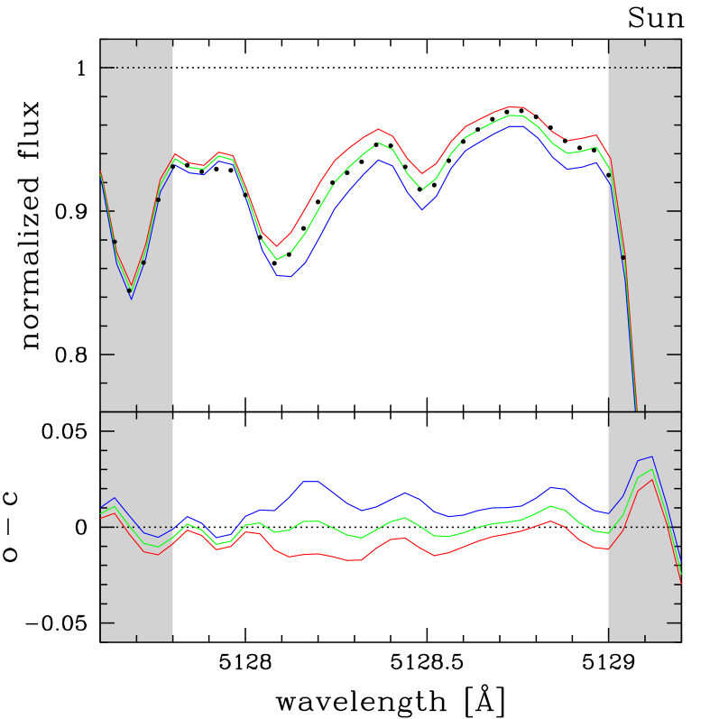
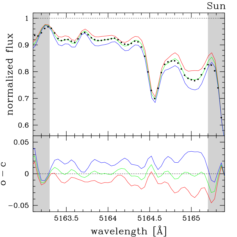
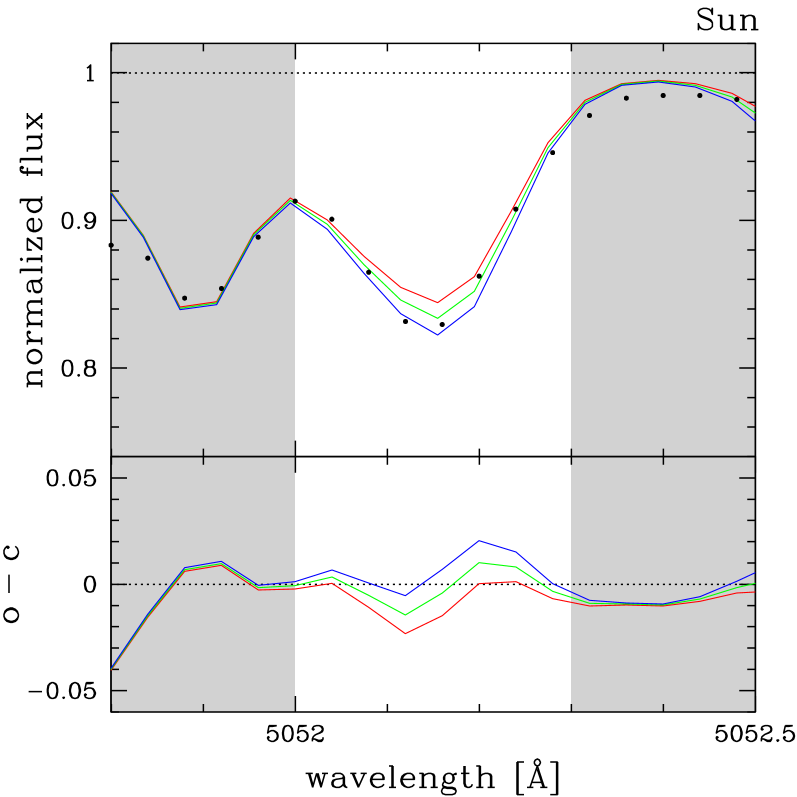
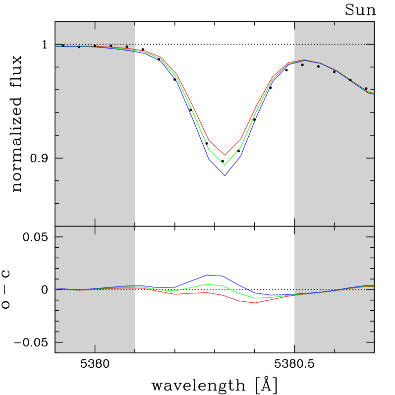
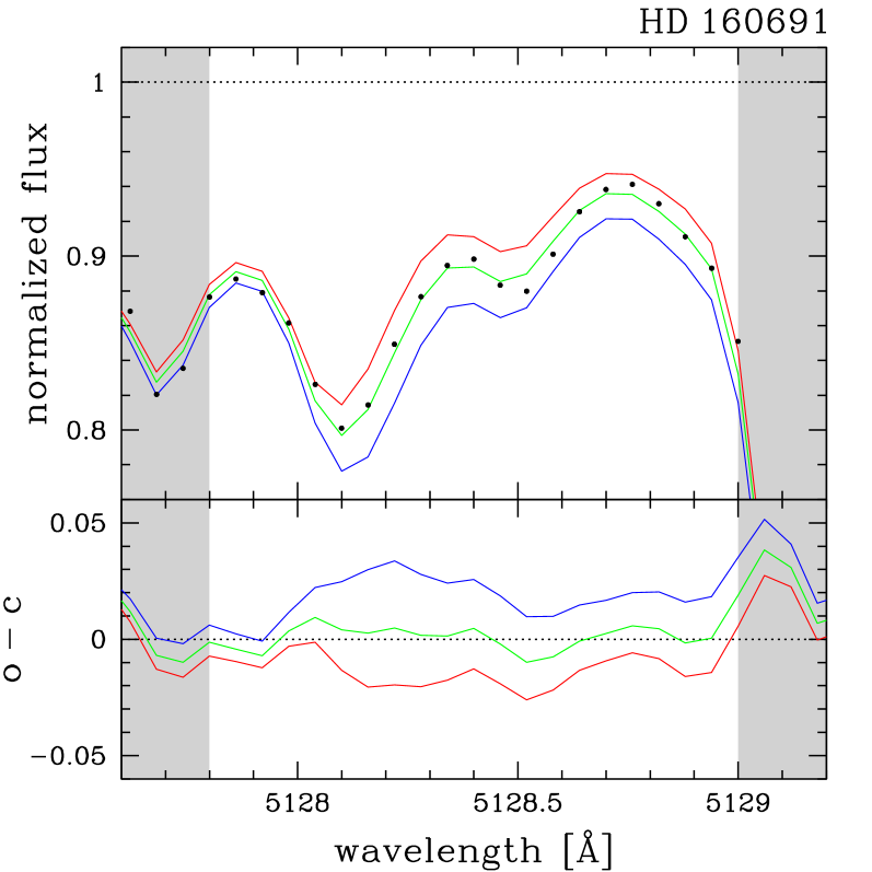
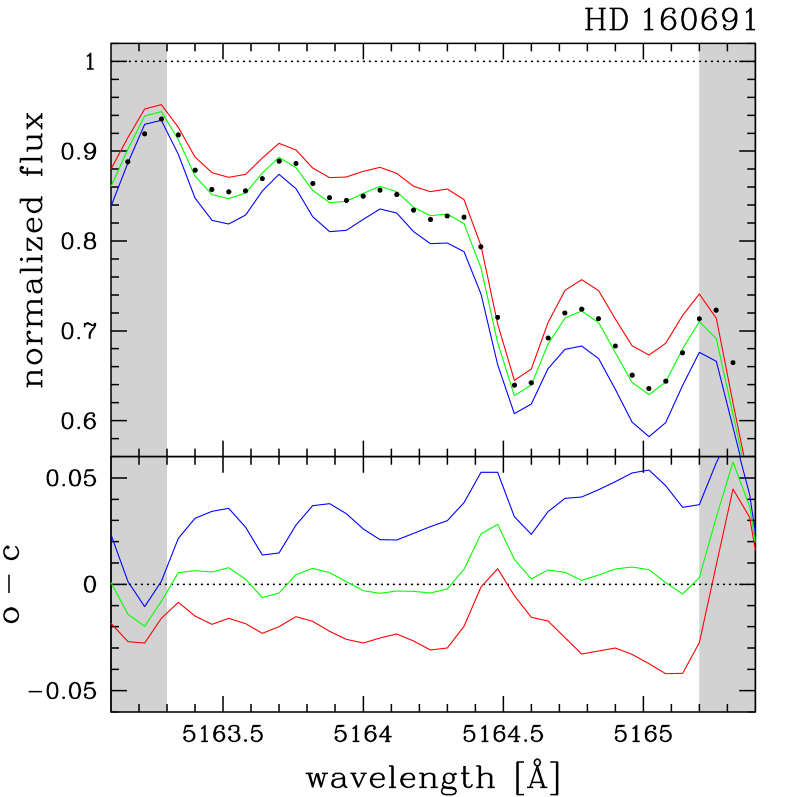
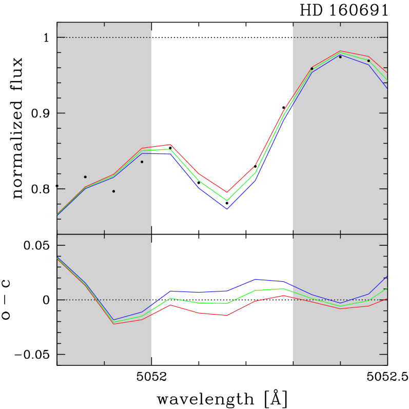
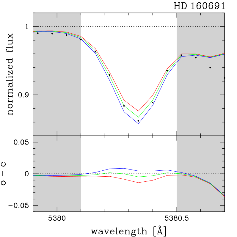
Figure 2: Spectral synthesis of the ${\rm C}_{2}$ molecular band regions ($\lambda$5128 and $\lambda$5165) and of the C atomic lines ($\lambda$5052.2 and $\lambda$5380.3) for Ganymede of the second observation run (top panels) and for one metal-rich star of the first run, HD 160691 (bottom panels). The solid lines represent three models with different values of [C/Fe]: $-$0.05 (red), 0.0 (green), and +0.05 dex (blue). The differences between observed (dots) and computed spectra (o$-$c) are also shown in the bottom of each panel.

The star HD 128620 is the primary component ($V$ = $-$0.01) of the $\alpha$ Cen triple system. The $T_{\rm eff}$ determination for very bright stars using photometric colours is normally considered risky due to systematic effects that may affect the results (such as non-linearity and detector dead time) and also, in the case of this system, due to a possible contamination by the companion. For this reason, we preferred do not include this star in our $T_{\rm eff}$ estimates based on the photometric indices. Nevertheless, our spectroscopic determination for $\alpha$ Cen A, $T_{\rm eff}^{\rm exc}$ = 5857 $\pm$ 30 K, is in good agreement with the photometric determination performed by Porto de Mello et al. (2008), $T_{\rm eff}$ = 5794 $\pm$ 34 K.

Concerning the uncertainties in $T_{\rm eff}^{\rm phot}$, on the one hand, the internal error of the weighted mean, computed using the standard deviations in the four photometric calibrations, is 31 K. On the other hand, the mean value of the standard deviations around $T_{\rm eff}^{\rm phot}$  (i.e., the dispersion of the four values of temperature around the weighted mean) is 41 K. Therefore, in this work we adopted $\sigma$($T_{\rm eff}^{\rm phot}$) = 40 K as the internal uncertainty in our photometric effective temperatures. This uncertainty intrinsically takes into account the errors in the colour indices themselves.

The stellar effective temperature can also be estimated by modelling the wing profile of the H$\alpha$ line, which is very sensitive to changes in this parameter. Lyra & Porto de Mello (2005) applied this method to solar neighbourhood stars, and values of $T_{\rm eff}^{{\rm H}\alpha}$ for our sample were used as a third $T_{\rm eff}$ indicator, with an uncertainty $\sigma$($T_{\rm eff}^{{\rm H}\alpha}$) = 50 K.

3.5 Carbon abundance from spectral synthesis

The carbon abundance was derived using the spectral synthesis method applied to molecular lines of electronic-vibrational band heads of the ${\rm C}_{2}$ Swan System at $\lambda$5128 and $\lambda$5165, and also to C atomic lines at $\lambda$5052.2 and $\lambda$5380.3. To reproduce the atomic and molecular absorption lines in the observed spectra of the sample stars, the MOOG spectral synthesis code, developed by Chris Sneden (University of Texas, USA), was used. The synthetic spectra were computed in steps of 0.02 Å, also taking into account the continuum opacity contribution in ranges of 0.5 Å. The Unsöld approximation multiplied by 6.3 was adopted in the calculations of the line damping parameters.

The model atmospheres are the same used in the spectroscopic analysis. They also include the micro-turbulence velocity and the elemental abundances of each star, both assumed to be constant in all layers. For any element X for which no abundance was determined in this work, we adopted the metallicity of the respective star to set the [X/H] ratio.

The atomic and molecular line parameters used to compute the synthetic spectra are: the central wavelength, the $gf$ values, the lower-level excitation potential, and the constant of dissociation energy $D_{0}$ (only for molecular features). Atomic and molecular data were taken, respectively, from the Vienna Atomic Line Database – VALD (Kupka et al. 1999, 2000; Piskunov et al. 1995; Ryabchikova et al. 1997) and from Kurucz (1992). In addition to ${\rm C}_{2}$, the spectral regions studied also include MgH molecular features that may contribute to the continuum formation. The oscillator strengths of ${\rm C}_{2}$ and MgH lines were revised according to the normalisation of the Hönl-London factors (Whiting & Nicholls 1974).

To account for the spectral line broadening, the synthetic spectra were computed by means of the convolution with three input parameters: $i)$ the spectroscopic instrumental broadening; $ii)$ the limb darkening of the stellar disc; and $iii)$ a composite of velocity fields, such as rotation velocity and macro-turbulence broadening, named $V_{\rm broad}$. The instrumental broadening was estimated by means of the FWHM of thorium lines present in Th-Ar spectra observed at the CTIO. The linear limb-darkening coefficient (on average $u\sim 0.7$ for all the sample stars) was individually estimated by interpolation of $T_{\rm eff}^{\rm exc}$ and $\log{g_{\rm ion}}$ in Table 1 of Díaz-Cordovéz et al. (1995). As a first estimate of $V_{\rm broad}$, the projected rotation velocity (v$\sin{i}$) of the stars was used, which was computed based on the profile of four isolated Fe I lines ($\lambda$5852.2, $\lambda$5855.1, $\lambda$5856.1, and $\lambda$5859.6) in the spectra. Small corrections in $V_{\rm broad}$ were applied when needed according to an eye-trained inspection of the synthetic spectra. The final values are listed in Table 5, where they can be compared to the stellar age and the chromospheric activity level.

Figure 2 shows two examples of synthetic spectra of the ${\rm C}_{2}$ molecular band regions around $\lambda$5128 and $\lambda$5165, and of the C atomic lines at $\lambda$5052.2 and $\lambda$5380.3 for the sunlight spectrum reflected by Ganymede (second observation run) and for the metal-rich star HD 160691. The spectral synthesis was first applied to the Ganymede spectra of both runs, then the $gf$ values of some atomic and molecular lines were revised when needed, and finally the synthesis was applied to the other stars, treated according to their observation runs. For each case, the best fit was obtained through the minimisation of the $rms$ between observed and synthetic spectra.

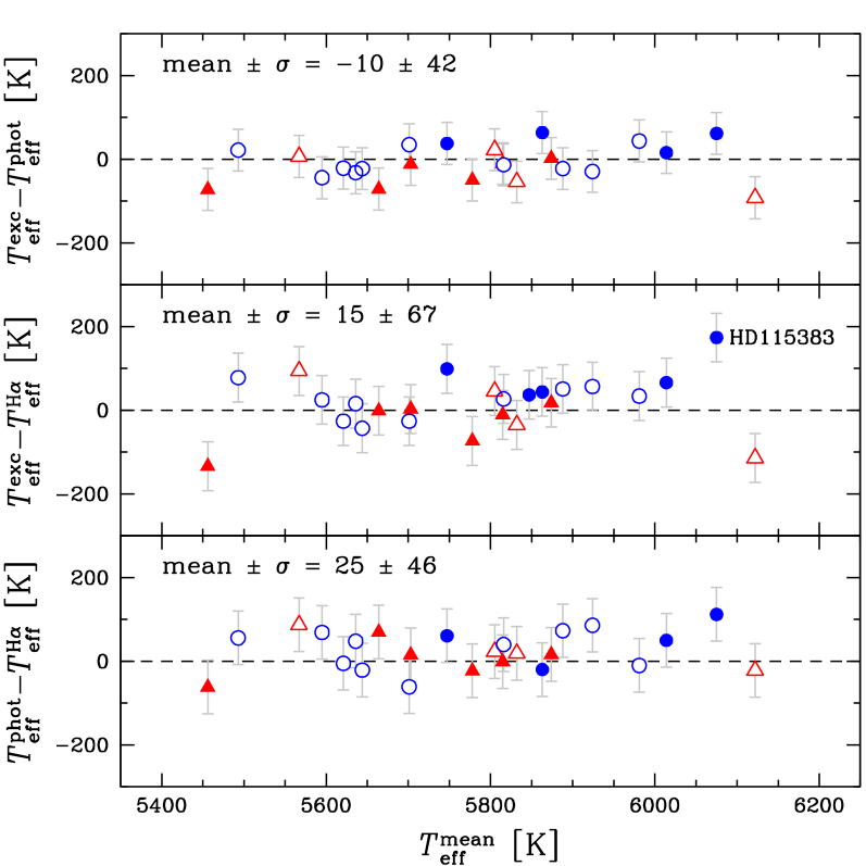
Figure 3: Comparisons of the three effective temperature indicators: the excitation vs. photometric (top panel), excitation vs. H$\alpha$ (middle panel), and photometric vs. H$\alpha$ (bottom panel) temperatures. The symbols represent the stellar groups defined in Sect. 5 (see Fig. 6).

In order to estimate the uncertainties in the [C/Fe] abundance determination, we performed a spectral synthesis of the most prominent molecular band used ($\lambda$5165) adopting model atmospheres perturbed by the errors estimated for the atmospheric parameters. This procedure resulted in: $\pm$0.03 dex due to the error in $T_{\rm eff}^{\rm exc}$; $\pm$0.01 dex due to the error in [Fe/H]; $\pm$0.02 dex due to the error in $\xi$; and $\pm$0.03 dex due to the error in $\log{g_{\rm ion}}$. The uncertainties related to errors in $V_{\rm broad}$  ($\sim$1.0 km s^-1 or smaller) and in the limb darkening coefficient are negligible. The quadratic sum of the individual contributions (also including a global error of 0.05 dex estimated based on the $rms$ minimisation of the solar spectrum) yields a total uncertainty $\sigma$([C/Fe]) = 0.07 dex.

4 Evolutionary, Kinematic, and orbital parameters

4.1 Mass and age determination

The evolutionary parameters mass and age were obtained by interpolation in the Yonsei-Yale (${\rm Y}^{2}$) evolutionary tracks and isochrones (Yi et al. 2001; Kim et al. 2002) drawn on the HR diagram and computed for different values of metallicity.

The luminosity used in the diagrams were calculated with parallaxes taken from the new reduction of the Hipparcos data (van Leeuwen 2007), bolometric corrections ($BC$) from Flower (1996), and an absolute bolometric magnitude for the Sun $M_{\rm bol}^{\odot}=4.75$ for $M_{\rm v}^{\odot}=4.82$. We estimated, for these nearby stars with precise parallaxes, a mean uncertainty of 0.01 dex in $\log(L/L_{\odot})$.

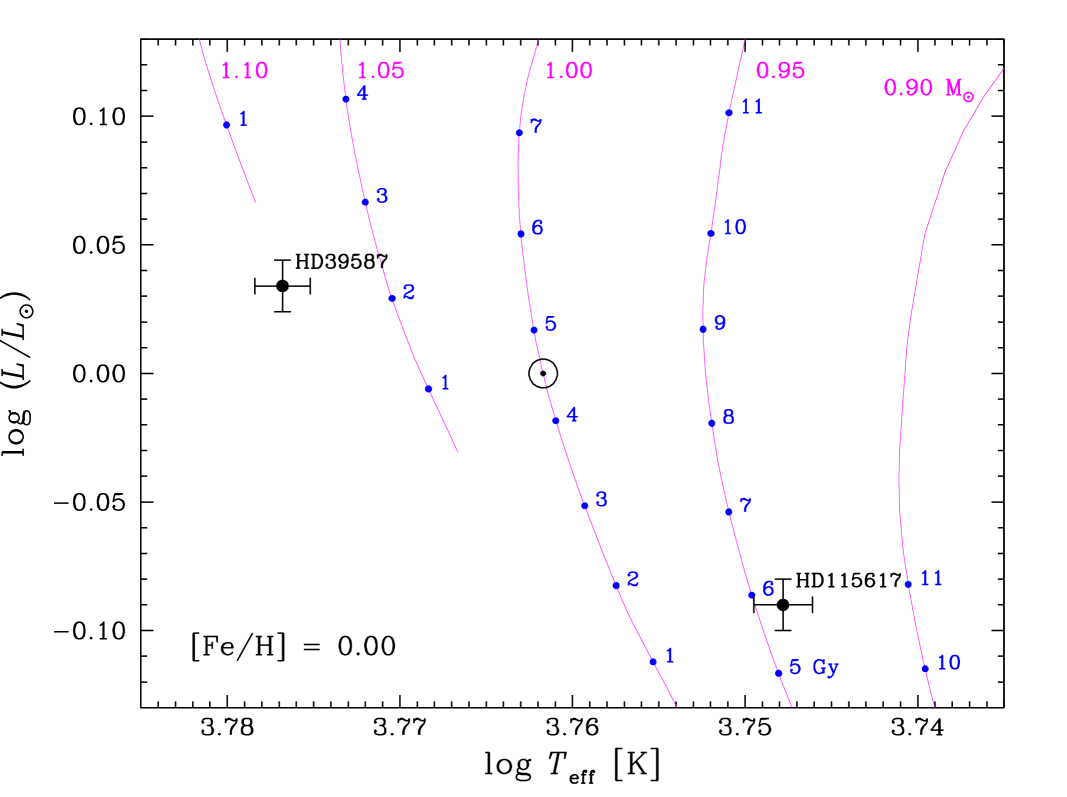
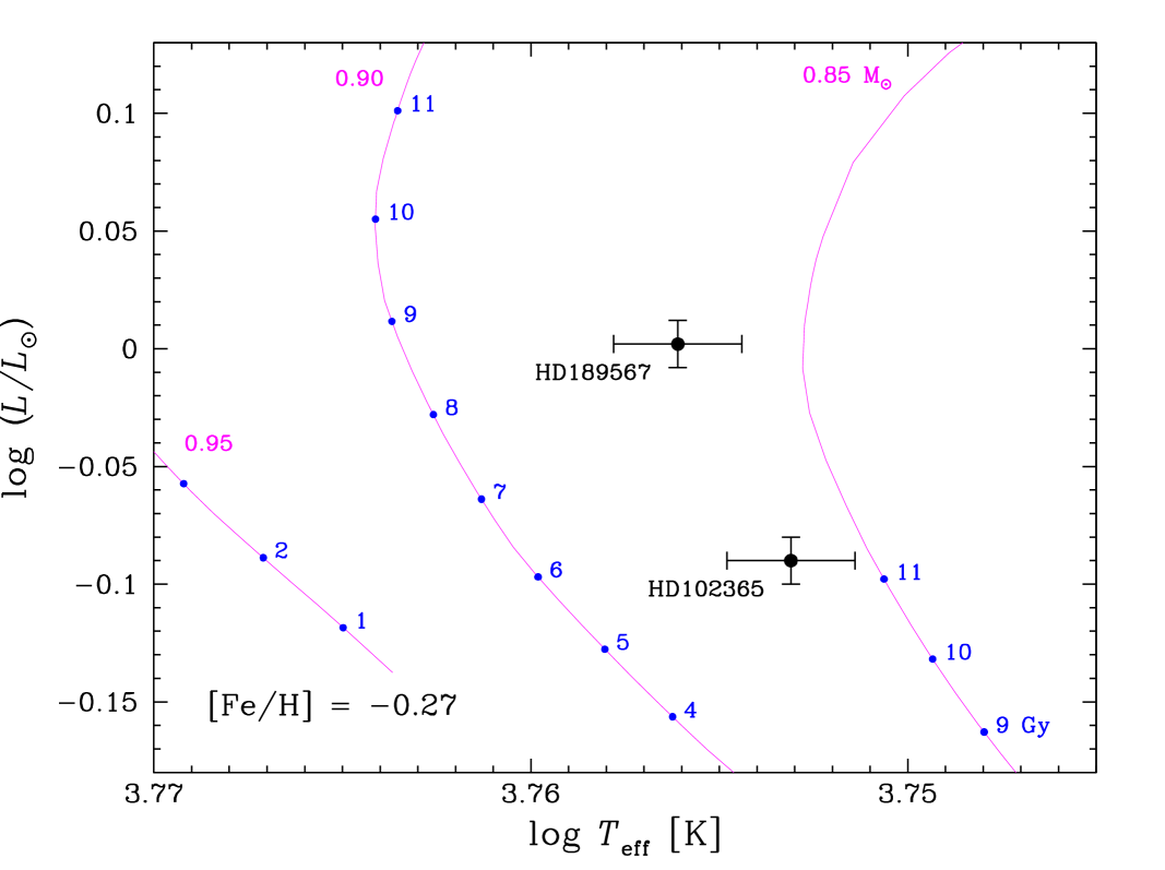
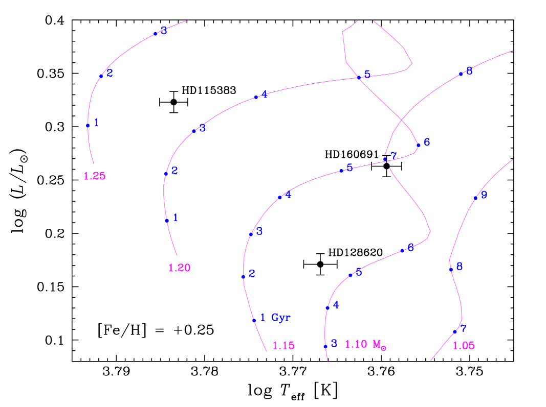
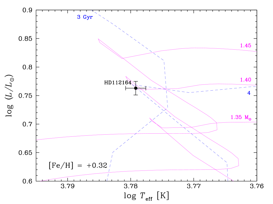
Figure 4: Evolutionary tracks (magenta solid lines) and isochrones (blue dots and dashed lines) from Yonsei-Yale, calculated for different values of metallicity, showing how to derive the stellar masses and ages. The ages in Gyr are indicated alongside the evolutionary tracks, for which the masses are indicated in ${\rm M}_{\odot}$. The Sun’s position for $T_{\rm eff}$ = 5777 K is also shown in the solar metallicity panel (top-left corner).

The effective temperature is a weighted mean ($T^{\rm mean}_{\rm eff}$) of the excitation, photometric, and H$\alpha$ temperatures. The weights are given by $1/\sigma^{2}$ for $\sigma$($T_{\rm eff}^{\rm exc}$) = 30 K, $\sigma$($T_{\rm eff}^{\rm phot}$) = 40 K, and $\sigma$($T_{\rm eff}^{{\rm H}\alpha}$) = 50 K, obtained as described in Sect. 3.2 and 3.4. The uncertainty of the weighted mean is 22 K, calculated using these three values of $\sigma$. On the other hand, the standard deviations of the three values of temperature around the weighted mean is 29 K. Therefore, we conclude that our estimates of effective temperature based on the three indicators agree with each other very well (see the comparison in Fig. 3) and that the mean value has a mean internal error $\sigma(T^{\rm mean}_{\rm eff})$ = 30 K.

Porto de Mello et al. (2008) determined the effective temperature of $\alpha$ Cen A (HD 128620) and B also using the excitation, photometric, and H$\alpha$ approaches. They found a good agreement for $\alpha$ Cen A, a solar temperature star. However, for $\alpha$ Cen B ($T_{\rm eff}$ $\sim$5200 K), the excitation effective temperature is about 100-150 K higher than the photometric and the H$\alpha$ counterparts, which the authors attributed to non-LTE effects. Although the agreement for the coolest and hottest stars in our sample is not that good, especially in the comparison of excitation and H$\alpha$ temperatures, Fig. 3 does not show any systematic difference among the three indicators, and the differences are nonetheless within 2$\sigma$ for all the $T_{\rm eff}$ range (only HD 115383 has $T_{\rm eff}^{\rm exc}$ larger than $T_{\rm eff}^{{\rm H}\alpha}$ by 3$\sigma$). This confirms that 1D LTE model atmospheres may adequately represent solar-type stars, at least in a differential analysis relative to the Sun.

We remind that the temperature used in our abundance analyses (based on the equivalent widths or synthesis of spectral features) was the excitation effective temperature, which better characterises the temperature radial profile in the stellar photosphere and the formation of absorption lines in the emergent spectrum. On the other hand, to better represent the luminosity of a star and to account for any possible effect due to small deviations from LTE, we adopted the weighted mean of the three temperature indicators.

The stars were grouped according to their values of metallicity (12 groups from [Fe/H] = $-$0.32 to +0.32 dex) and then their masses and ages were computed using evolutionary tracks and isochrones for each stellar group. The difference in metallicity between each star and its respective HR diagram is not greater than 0.02 dex. A few examples for some metallicities are shown in Fig. 4. To reproduce the Sun’s position in the diagrams, adopting $T_{\rm eff}$ = 5777 K and $age$ = 4.53 Gy (Guenther & Demarque 1997), the evolutionary tracks and isochrones were displaced in $\log(T_{\rm eff})$ and $\log(L/L_{\odot})$ by 0.001628 ($\sim$22 K in $T_{\rm eff}$) and 0.011, respectively. These values are, at any rate, of the same order or smaller than the uncertainties on these parameters.

As an independent check, we calculated the evolutionary surface gravity using the values of mass and effective temperature obtained, which we called $g_{\rm evol}$, using the following equation:

$$\log\frac{g_{\rm evol}}{g_{\odot}}=\log\frac{M}{M_{\odot}}+4\log\frac{T^{\rm mean}_{\rm eff}}{T_{\rm eff}^{\odot}}+0.4(M_{\rm bol}-M_{\rm bol}^{\odot})$$ (7)

where $M_{\rm bol}$ is the absolute bolometric magnitude for the stars. The values of $\log{g_{\rm evol}}$ are listed in Table 2 together with the ionisation surface gravity. They are in very good agreement, having a dispersion of only 0.09 dex, smaller than the uncertainty of 0.13 dex estimated for $\log{g_{\rm ion}}$.

4.2 Galactic velocities, distance, and eccentricity

The kinematic properties of our sample were investigated by computing the Galactic velocity components $U_{\rm LSR}$, $V_{\rm LSR}$, and $W_{\rm LSR}$  (see Fig. 5) with respect to the Local Standard of Rest (LSR). We developed a code that uses equations of Johnson & Soderblom (1987), parallaxes and proper motions both from the new reduction of the Hipparcos data, and radial velocities from Holmberg et al. (2007), Torres et al. (2006) for HD 114613, and Santos et al. (2004) for HD 160691. For the Sun, the adopted values of $U_{\rm LSR}$, $V_{\rm LSR}$, and $W_{\rm LSR}$ are 10.0, 5.3, and 7.2 km s^-1, respectively (Dehnen & Binney 1998).

The mean orbital distance from the Galactic centre ($R_{\rm m}$) and the orbital eccentricity ($e$) were also considered in our analysis (see Fig. 5), where $e$ = ($R_{\rm a}$$-$ $R_{\rm p}$)/($R_{\rm a}$+ $R_{\rm p}$) and $R_{\rm m}$ = ($R_{\rm a}$+ $R_{\rm p}$)/2 were computed using the perigalactic ($R_{\rm p}$) and the apogalactic ($R_{\rm a}$) orbital distances from the Geneva-Copenhagen survey (Holmberg et al. 2009). For the Sun, the adopted values are $e$ = 0.06 and $R_{\rm m}$ = 8 kpc.

5 Tree clustering analysis

We looked for statistically significant abundance groups in our sample using a hierarchical clustering analysis. To avoid missing abundance values, the analysis uses only those elements having abundances measured for all stars and was applied to the [X/H] abundance space.

We used the complete linkage method for the hierarchical clustering (Everitt et al. 2001) and euclidean distances as measures of dissimilarities in this abundance space. A hierarchical clustering algorithm works by joining similar objects in a hierarchical structure. Initially, each object is assigned to its own cluster. The algorithm proceeds iteratively, joining the two most similar clusters in each pass until there is just a single cluster. The resulting hierarchy of clusters for our data is shown in Fig. 6 (upper panel) as a dendrogram. In this plot, the most similar objects are linked together in the bottom forming clusters, which are then iteratively linked together in pairs by similarity. The vertical axis in a dendrogram measures the dissimilarity between each individual or cluster. Since we used euclidean distances in the [X/H] abundance space, the units of this axis is dex, although it measures the total dissimilarity in this abundance space and not in a single variable.

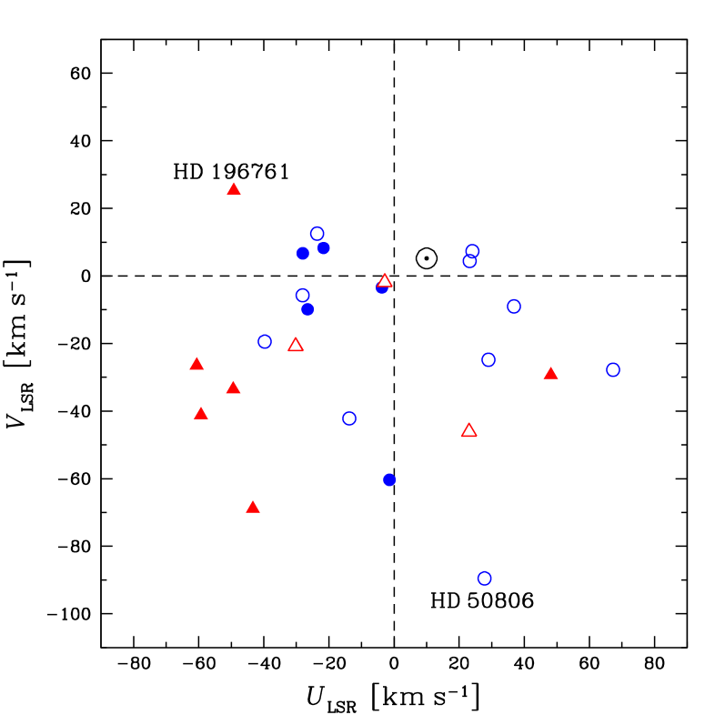
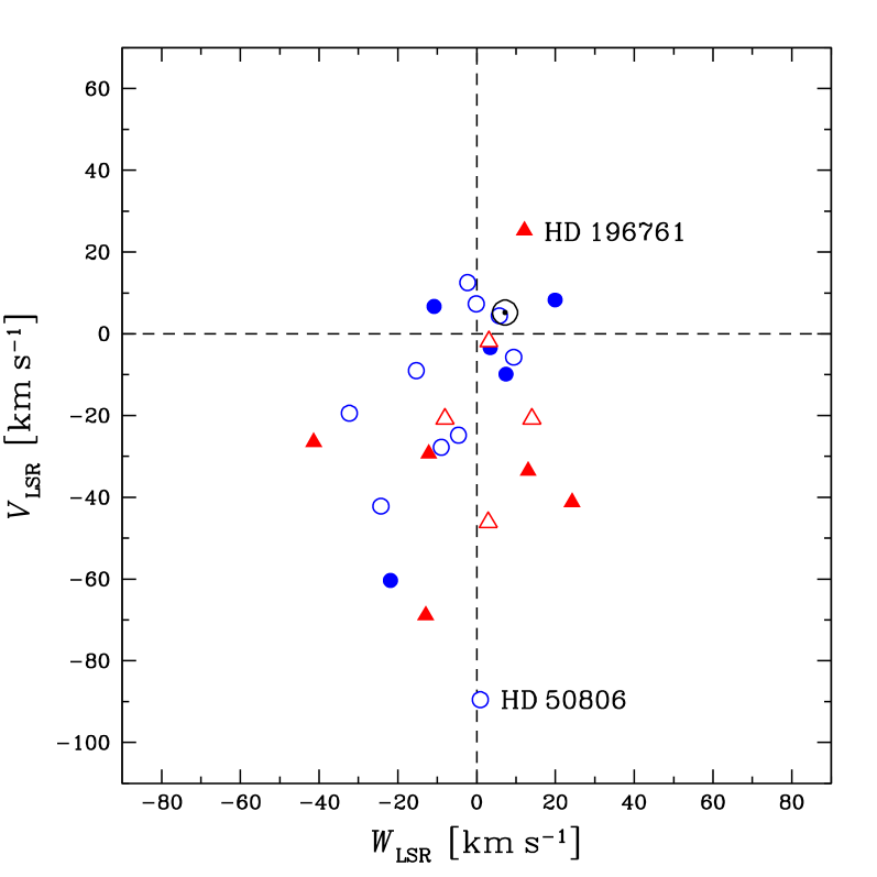
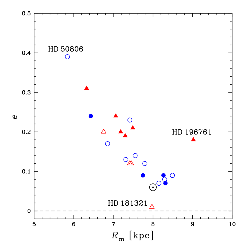
Figure 5: Galactic velocity components (left and middle panels) and orbital eccentricity as a function of the mean orbital distance from the Galactic centre (right panel) for the sample stars and the Sun. The symbols represent the stellar groups defined in Sect. 5.

Clusters can be defined by specifying a reasonable total dissimilarity value for pruning the dendrogram. There is no unambiguous or optimal way for defining this pruning value, especially because the clusters found depend on the clustering method and cluster shapes. Since our sample is quite small, we arbitrarily decided to prune our dendrogram at the total dissimilarity of 0.9 dex, which is shown in Fig. 6 by the dashed red line. This pruning value was chosen in order to have four more or less equally populated clusters. Considering the size of our sample, less than four clusters would simply limit our discussion to poor against rich stars, while a larger number of clusters would make such an analysis meaningless.

The average $\langle$[X/H]$\rangle$ behaviour of the four clusters for each element considered in this analysis is shown in the middle panel of Fig. 6. Two of these clusters have over-solar abundances, with averages +0.26 and +0.06 dex for all the elements, whereas the two others have under-solar abundance values, with averages $-$0.06 and $-$0.24 dex. We can observe in the figure that the elemental abundance patterns of the metal-poor and metal-rich groups are distinct between each other. In particular, it seems to exit a chemical distinction even between the two intermediate groups: the under-solar intermediate group has an abundance pattern that roughly follows the element by element pattern of the metal-poor group, whereas the pattern of the over-solar intermediate group resembles the scaled-solar mixture.

The clustering analysis we have presented was tentatively based on biological ideas of evolving species, in the sense that the material the stars came from is continuously changing. For this reason we made use of [X/H] abundances ratios instead of [X/Fe]. We implicitly need the time evolution that [X/H] has, because we want a time hierarchy in the output groups. A similar analysis in the [X/Fe] space can still show groups, but the hierarchical relation between these groups in a dendrogram will not necessarily show evolutionary trends, because this variable is only indirectly linked with time. Notwithstanding, we have checked this, but the output groups show no meaningful interpretation in terms of chemical evolution or abundance ratio groups. The outcome could be different if the sample were larger, but this needs to be verified with another sample, what is beyond the scope of this paper. Nevertheless, we included in Fig. 6 (bottom panel) the average $\langle$[X/Fe]$\rangle$ behaviour of the stars clustered in the [X/H] parameter space. The small variation of $\langle$[X/Fe]$\rangle$ with respect to the solar values reinforces our point above: that for this specific small sample, the [X/Fe] parameter space is dynamically very narrow and does not favour a cluster analysis.

6 Results and discussion

Table 5 lists the evolutionary (mass and age), kinematic ($U_{\rm LSR}$, $V_{\rm LSR}$, and $W_{\rm LSR}$ velocities), and orbital (mean orbital distance from the Galactic centre and orbital eccentricity) parameters computed for the program stars. They are grouped following the tree clustering analysis performed in Sect. 5.

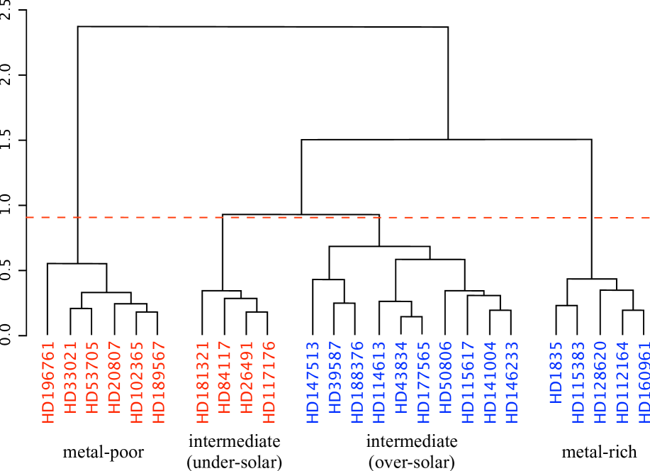
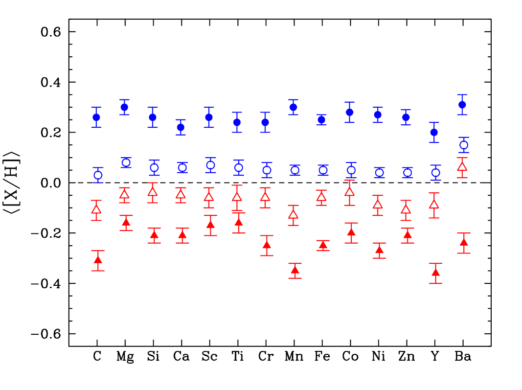
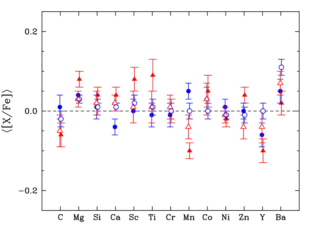
Figure 6: Dendrogram (upper panel) and mean abundance ratios $\langle$[X/H]$\rangle$ (middle panel) and $\langle$[X/Fe]$\rangle$ (bottom panel) for the four stellar groups from the tree clustering analysis (Sect. 5). They are classified as metal-poor ( $\blacktriangle$), intermediate abundance (under solar $\triangle$ or over solar $\circ$), or metal-rich ( $\bullet$) stars, and the same symbolism is adopted all over the paper. The dashed red line on the dendrogram represents a dissimilarity number of 0.9 dex.

The uncertainties in the mass and age determination may vary widely depending on the stellar position in the HR diagram. We made an estimate of these errors for a few representative stars in our sample (cool and hot dwarfs and subgiants). We took into account the errors estimated for $\log(L/L_{\odot})$, $\log(T_{\rm eff})$, and also [Fe/H] considering that the evolutionary tracks and isochrones are metallicity dependent. We found that the uncertainties in mass stand between 0.02 and 0.08 ${\rm M}_{\odot}$, whereas those in age vary from about 0.5 Gyr (or smaller) for evolved stars up to about 2.5 Gyr for cool main-sequence stars.

For HD 1835, HD 39587, HD 147513, and HD 181321 we determined an approximative value for their masses and an upper limit for their ages given their position in the HR diagram (close to the Zero Age Main Sequence). Indeed, these are very young stars: one of them, HD 1835, is likely a member of the Hyades star cluster ($\sim$600 Myr) according to López-Santiago et al. (2010); two others, HD 39587 (Soderblom & Mayor 1993; Fuhrmann 2004) and HD 147513 (Soderblom & Mayor 1993; Montes et al. 2001) belong to the Ursa Major moving group of $\sim$300 Myr (see also Castro et al. 1999); and HD 181321 is a member of the Castor moving group ($\sim$200 Myr) according to Montes et al. (2001). For these four stars, we adopted the ages of their respective moving group in our study.

The stars HD 112164 and HD 160691, indicated by asterisks (*) in Table 5, are located in a region of the HR diagram where successive evolutionary tracks and isochrones are superposed (see example in Fig. 4). Therefore, their mass and age determination may yield larger uncertainties: $\lesssim$ 0.12 ${\rm M}_{\odot}$ and $\lesssim$ 0.7 Gyr for HD 112164, and $\lesssim$ 0.04 ${\rm M}_{\odot}$ and $\lesssim$ 1.0 Gyr for HD 160691.

The $U_{\rm LSR}$, $V_{\rm LSR}$, and $W_{\rm LSR}$ velocities have a typical uncertainty of 0.3 km s^-1 or smaller. An exception is the star HD 188376, for which the large errors (2.5, 1.1, and 1.8 km s^-1, respectively) are due to a large uncertainty in its parallax. The level of activity in the chromosphere of the stars, which is related to their age, was also investigated. The table lists the flux in the centre of the H$\alpha$ line ($F^{\prime}_{{\rm H}\alpha}$), computed by Lyra & Porto de Mello (2005) and used as a chromospheric activity indicator (the larger the value of $F^{\prime}_{{\rm H}\alpha}$, the higher the level of chromospheric activity). The uncertainty for this parameter is 0.5$\times 10^{5}$ erg cm^-2 s^-1.

We note that a few stars in our sample have at least one planetary companion detected. They are HD102365, HD115617, HD117176, HD147513, and HD160691 (see The Extrasolar Planets Encyclopaedia: http://exoplanet.eu). Comparisons of properties of stars with and without planets are frequently published. In the analysis performed in this paper, however, no peculiar information distinguishing the two populations has been found.

6.1 Elemental abundances

Table 10 lists the chemical abundances relative to iron [X/Fe] obtained for the elements studied. For some elements of some stars, the abundance determination was not possible due to the poor quality or the weakness of their spectral lines (empty fields in the table). The carbon abundance ratios [C/Fe] are shown in Table 6.

We also computed the mean abundance ratios $\langle$[X/Fe]$\rangle$ of the following groups of elements: $i)$ two groups of light metals: (Mg, Si) and (Ca, Sc, Ti); $ii)$ two groups of the iron peak: (V, Cr, Co, Ni) and (Mn, Cu); $iii)$ light elements from the s-process: (Sr, Y, Zr), to which we refer as ls; and $iv)$ heavy elements from the s-process: (Ba, Ce, Nd), referred to as hs (see Table 7). They were grouped either because they have possibly the same nucleosynthetic origin or because they share a similar behaviour in the diagrams. The abundance ratio between heavy and light elements from the s-process, [hs/ls] = [hs/Fe] $-$ [ls/Fe], was also calculated.

Figure 7 shows diagrams with the abundance ratios of the program stars for individual elements and nucleosynthetic groups. The uncertainties are listed in Tables 3 and 7. As for the individual elements, the estimated errors are compared to the dispersions around the mean for groups having at least two elements. For each group of each observation run (represented by the stars HD 146233 and HD 26491), the larger values were adopted to be the uncertainties in the grouped abundance ratios. In Fig. 7, the stars are represented by different symbols according to the tree clustering analysis performed in Sect. 5.

The star HD 1835 is enriched in Ca, Sr, and Ba. The mean value of all s-process elements also suggests an over-solar abundance. Sm, the only r-process element analysed here, shows an under-solar abundance of $-$0.3 dex, but with a large error. As already mentioned, this is a very young star, a probable member of the Hyades star cluster of age $\sim$600 Myr, which is in agreement with its high level of chromospheric activity indicated by $F^{\prime}_{{\rm H}\alpha}$ in Table 5.

Table 5: Evolutionary, kinematic, and orbital parameters, separating the stars according to the classification of Sect. 5. The H$\alpha$ fluxes ($F^{\prime}_{{\rm H}\alpha}$), from Lyra & Porto de Mello (2005), are given in units of $10^{5}$ erg cm^-2 s^-1. The mean distance from the Galactic centre ($R_{\rm m}$) and the orbital eccentricity ($e$) are from Holmberg et al. (2009). The asterisk (*) indicates stars adjacent to superposed evolutionary tracks and isochrones on the HR diagram.

	$T^{\rm mean}_{\rm eff}$ [K]	[Fe/H]		$\log L/{L_{\odot}}$		$M/{M_{\odot}}$		$age$ [Gyr]		$V_{\rm broad}$ [km s-1]		$F^{\prime}_{{\rm H}\alpha}$		$U_{\rm LSR}$ [km s-1]		$V_{\rm LSR}$ [km s-1]		$W_{\rm LSR}$ [km s-1]		$R_{\rm m}$ [kpc]	$e$
Sun	5777	0	.00	0	.00	1	.00	4	.53	1	.8	3	.4	10	.0	5	.3	7	.2	8.00	0.06
metal-poor stars:
HD 20807	5874	$-$0	.22	$-$0	.02	0	.96	4	.2	$<$	2	3	.6	$-$59	.3	$-$41	.2	24	.2	7.06	0.24
HD 33021	5778	$-$0	.20	0	.35	0	.98	10	.1	4	.1	3	.8	48	.2	$-$29	.3	$-$12	.2	7.30	0.19
HD 53705	5815	$-$0	.22	0	.14	0	.93	10	.1	4	.0	1	.9	$-$43	.4	$-$68	.9	$-$12	.9	6.33	0.31
HD 102365	5664	$-$0	.28	$-$0	.09	0	.86	10	.1	$<$	2	2	.1	$-$49	.4	$-$33	.5	13	.1	7.18	0.20
HD 196761	5456	$-$0	.32	$-$0	.27	0	.80	10	.8	3	.3	4	.9	$-$49	.2	25	.3	12	.1	9.02	0.18
HD 189567	5703	$-$0	.27	0	.00	0	.87	11	.9	4	.4	2	.9	$-$60	.6	$-$26	.5	$-$41	.4	7.49	0.21
intermediate abundance (under solar) stars:
HD 26491	5805	$-$0	.09	0	.13	0	.97	8	.5	3	.5	2	.1	$-$30	.2	$-$20	.8	$-$8	.0	7.42	0.12
HD 84117	6122	$-$0	.06	0	.29	1	.12	3	.9	5	.9	0	.0	$-$30	.2	$-$20	.8	14	.1	7.45	0.12
HD 117176	5567	$-$0	.04	0	.47	1	.08	8	.2	$<$	2	1	.5	23	.1	$-$46	.2	3	.0	6.75	0.20
HD 181321	5832	$-$0	.06	$-$0	.12	$\sim$1	.02	0	.2	12	.5	14	.2	$-$2	.9	$-$1	.9	3	.1	7.97	0.01
intermediate abundance (over solar) stars:
HD 39587	5981	0	.00	0	.03	$\sim$1	.10	0	.3	9	.0	10	.3	24	.0	7	.3	$-$0	.1	8.29	0.08
HD 43834	5636	0	.11	$-$0	.08	0	.99	3	.9	$<$	2	2	.8	29	.0	$-$24	.8	$-$4	.6	7.31	0.13
HD 50806	5621	0	.02	0	.35	1	.02	9	.9	2	.0	2	.8	27	.8	$-$89	.5	0	.9	5.84	0.39
HD 114613	5701	0	.15	0	.62	1	.26	5	.1	$<$	2	1	.7	$-$28	.1	$-$5	.7	9	.4	–	–
HD 115617	5595	0	.00	$-$0	.09	0	.94	6	.8	$<$	2	4	.2	$-$13	.8	$-$42	.2	$-$24	.3	6.85	0.17
HD 141004	5924	0	.03	0	.32	1	.10	6	.3	$<$	2	1	.6	$-$39	.7	$-$19	.4	$-$32	.3	7.55	0.14
HD 146233	5816	0	.05	0	.02	1	.03	3	.4	$<$	2	2	.7	36	.8	$-$9	.0	$-$15	.3	7.79	0.12
HD 147513	5888	0	.04	$-$0	.02	$\sim$1	.05	0	.3	$<$	2	7	.0	23	.2	4	.4	5	.8	8.15	0.07
HD 177565	5644	0	.08	$-$0	.06	1	.00	4	.2	2	.3	3	.8	67	.3	$-$27	.8	$-$9	.0	7.41	0.23
HD 188376	5493	0	.00	0	.90	1	.53	2	.7	$<$	2	0	.5	$-$23	.6	12	.5	$-$2	.3	8.49	0.09
metal-rich stars:
HD 1835	5863	0	.21	0	.00	$\sim$1	.15	0	.6	5	.9	7	.7	$-$26	.5	$-$9	.9	7	.4	7.74	0.09
HD 112164	6014	0	.32	0	.76	1	.40*	3	.5*	4	.6	1	.4	$-$1	.4	$-$60	.4	$-$21	.9	6.43	0.24
HD 115383	6075	0	.23	0	.32	1	.22	2	.9	7	.0	8	.0	$-$28	.1	6	.7	$-$10	.8	8.27	0.09
HD 128620	5847	0	.23	0	.17	1	.11	4	.4	$<$	2	4	.7	$-$21	.7	8	.3	19	.9	8.31	0.07
HD 160691	5747	0	.27	0	.26	1	.12*	6	.2*	$<$	2	2	.4	$-$3	.7	$-$3	.4	3	.4	–	–

Two other very young stars are HD 39587 and HD 147513, both members of the kinematic Ursa Major group. They are clearly overabundant in the s-process elements, especially Ba, and underabundant in C, which is in agreement with the results of Porto de Mello & da Silva (1997a) and Castro et al. (1999). These stars were proposed by Porto de Mello & da Silva (1997a) to be barium stars, originated in a phenomenon in which the more massive component of a binary system evolves as a thermally pulsing asymptotic giant branch (TP-AGB) star and the material produced in the He-burning envelope, enriched in s-process elements, is dredged-up to the surface and then accreted by its companion by wind mass transfer. The initially more massive star is now a white dwarf whereas the companion has become the primary barium star. At present, HD 39587 is a single-lined spectroscopic and astrometric binary, with a low mass companion of 0.15 ${\rm M}_{\odot}$ (König et al. 2002), and HD 147513 has a common proper motion companion, a DA2 white dwarf, at an angular separation of 345$\arcsec$ (Holberg et al. 2002). The barium-star scenario was not supported by Castro et al. (1999), who proposed that the two stars simply have usual Ba abundances for their age and that probably all the Ursa Major group members are Ba-enriched, either due to a primordial origin or because they are young (see discussion in Sect. 6.4).

HD 181321 and HD 188376 are two other Ba-rich stars. HD 188376 is the most evolved and massive star analysed here, clearly in the evolutionary stage of a subgiant. The other star, HD 181321, is the youngest and has the highest level of chromospheric activity in our sample. Indeed, our determination for $V_{\rm broad}$ is 12.5 km s^-1, indicating a fast-rotating star. It has solar atmospheric parameters, excepting a high value of micro-turbulence velocity ($\xi$ = 2.3 km s^-1). The kinematic and orbital parameters are also very close to the solar values. In other words, this star has, on the one hand, about the same effective temperature, metallicity, surface gravity, mass, Galactic orbit, and space velocities as the Sun. On the other hand, it is very young and significantly enriched in Ba, strengthening the relation between Ba abundance and age (see Sect. 6.4).

The high microturbulence velocity of the star HD 181321 is probably prompted by the strengthened convection and turbulence in its upper photosphere, which is subjected to large non-thermal energy influxes from the chromosphere. The UV radiation excess from the chromosphere of an active star can scape to the photosphere and cause departures from LTE due to an ionisation imbalance. The induced overionisation is commonly manifested by differences either in excitation and photometric effective temperatures, or in ionisation and evolutionary surface gravities (see Porto de Mello et al. 2008; Ribas et al. 2010). For HD 181321, our determination of $T_{\rm eff}^{\rm exc}$ and $T_{\rm eff}^{\rm phot}$ are in very good agreement with each other. Therefore, only the difference in surface gravity and the large value of microturbulence velocity are possible signs that an overionisation is taking place in the photosphere of this active star. A full non-LTE analysis and a photospheric and chromospheric modelling would probably settle the issue, but this goes beyond the scope of this paper.

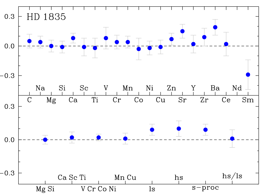
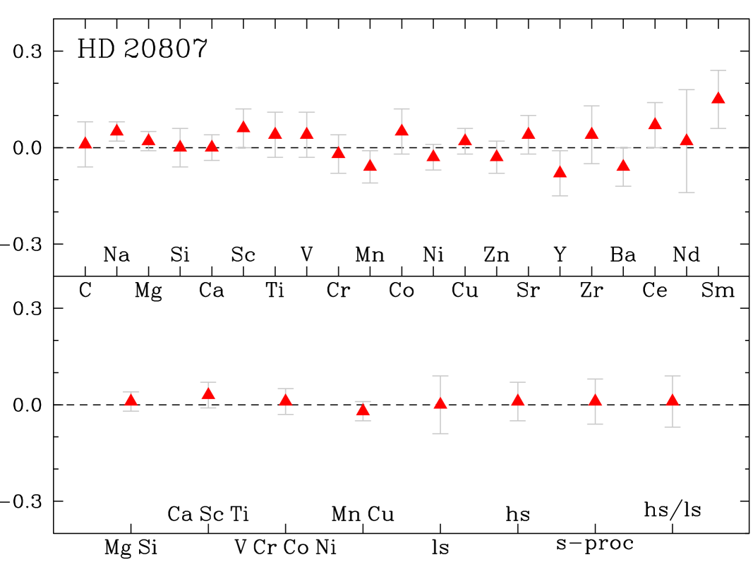
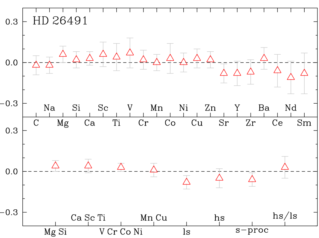
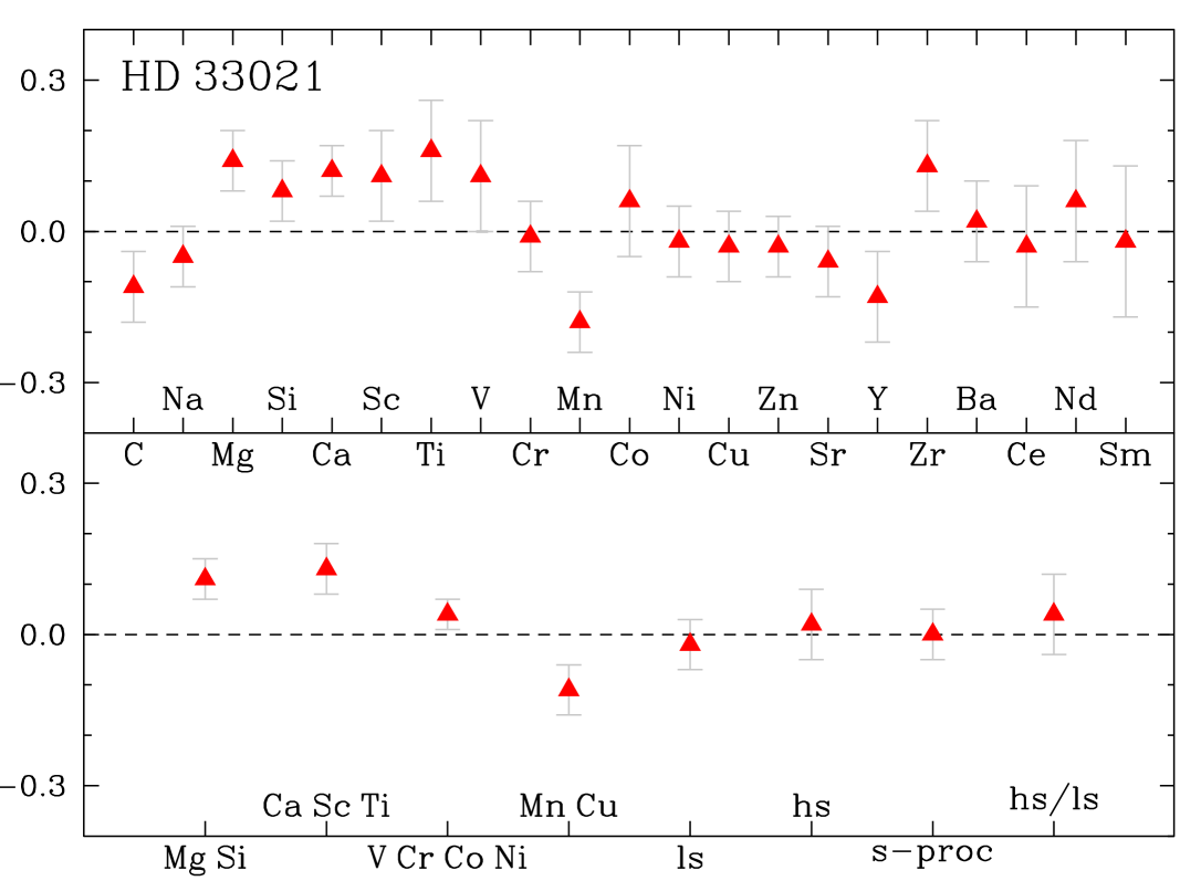
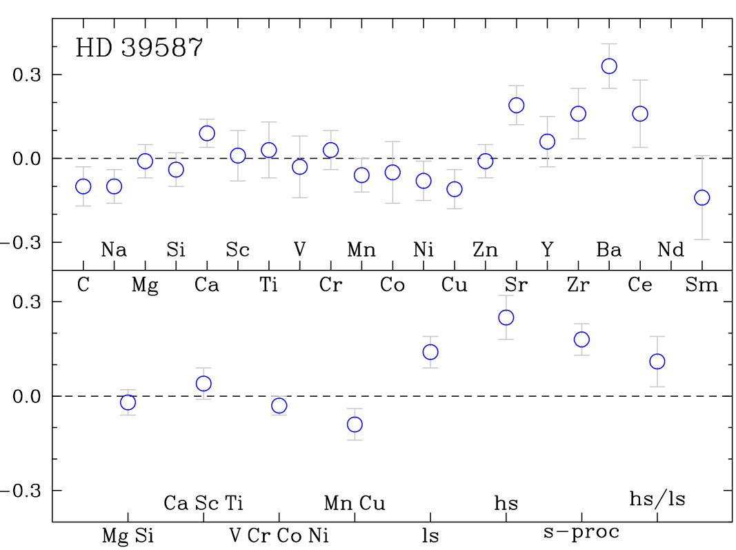
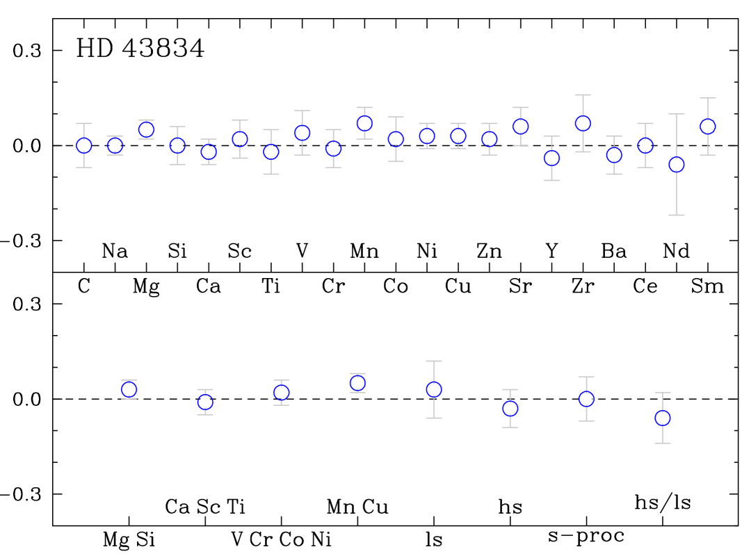
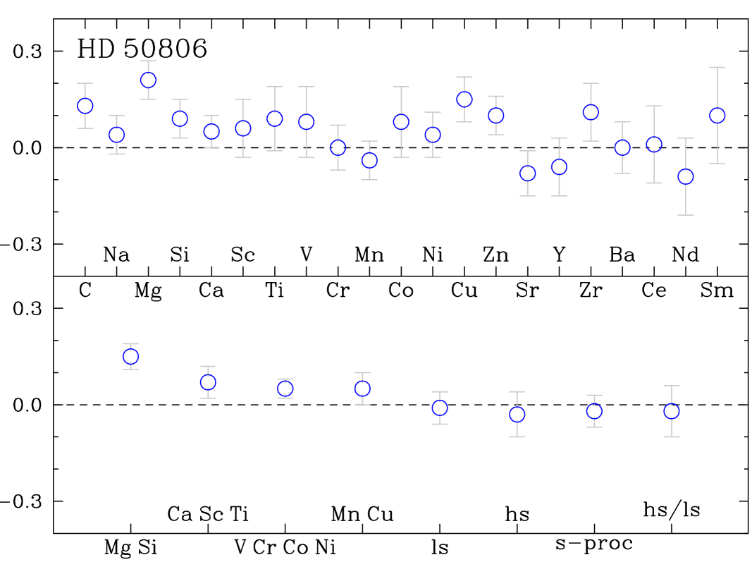
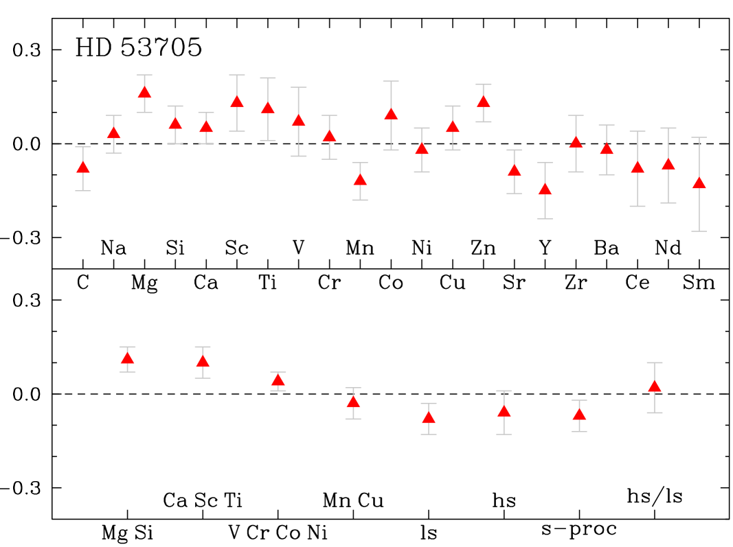
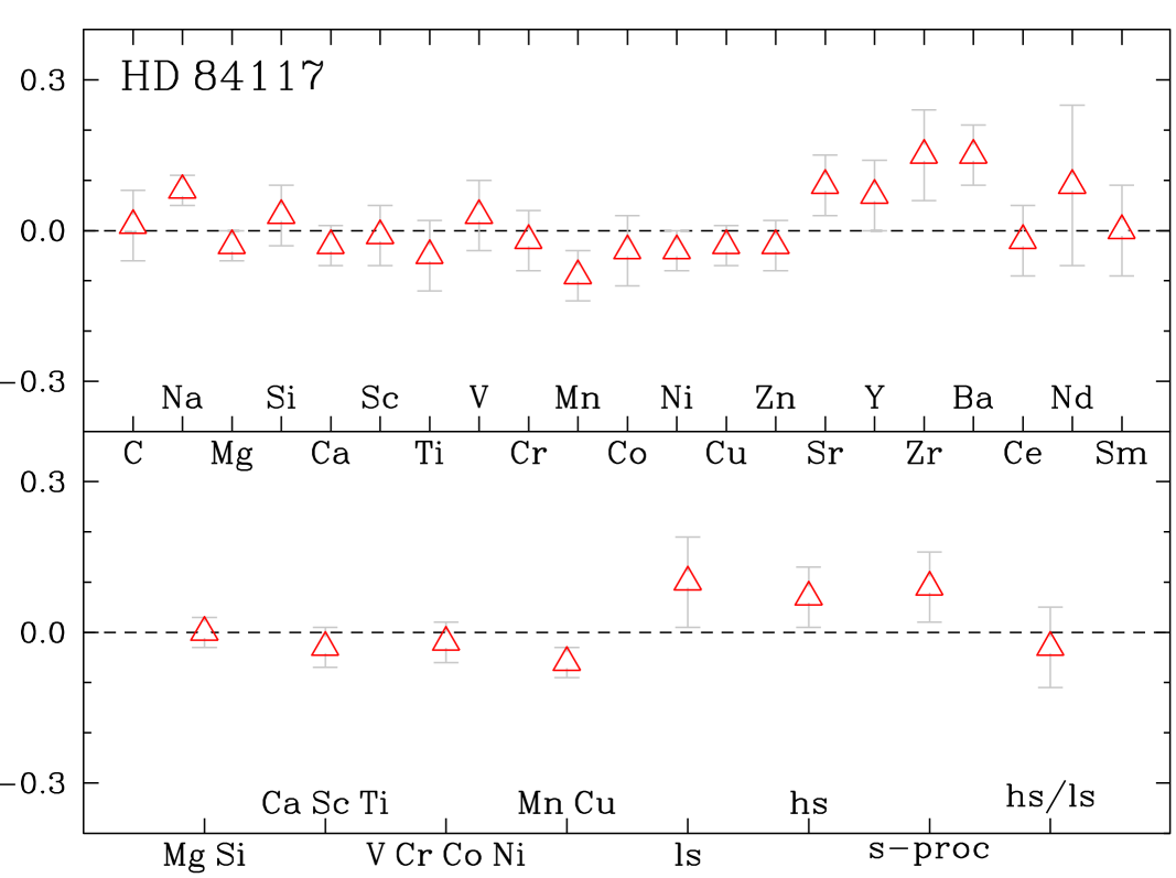
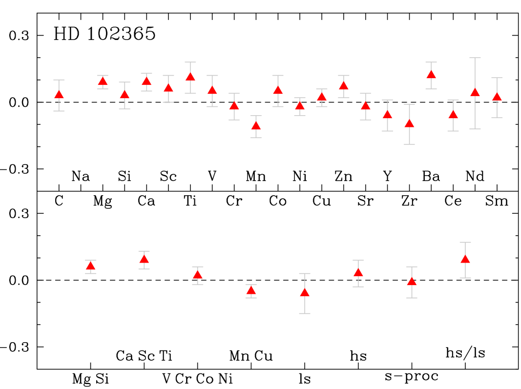
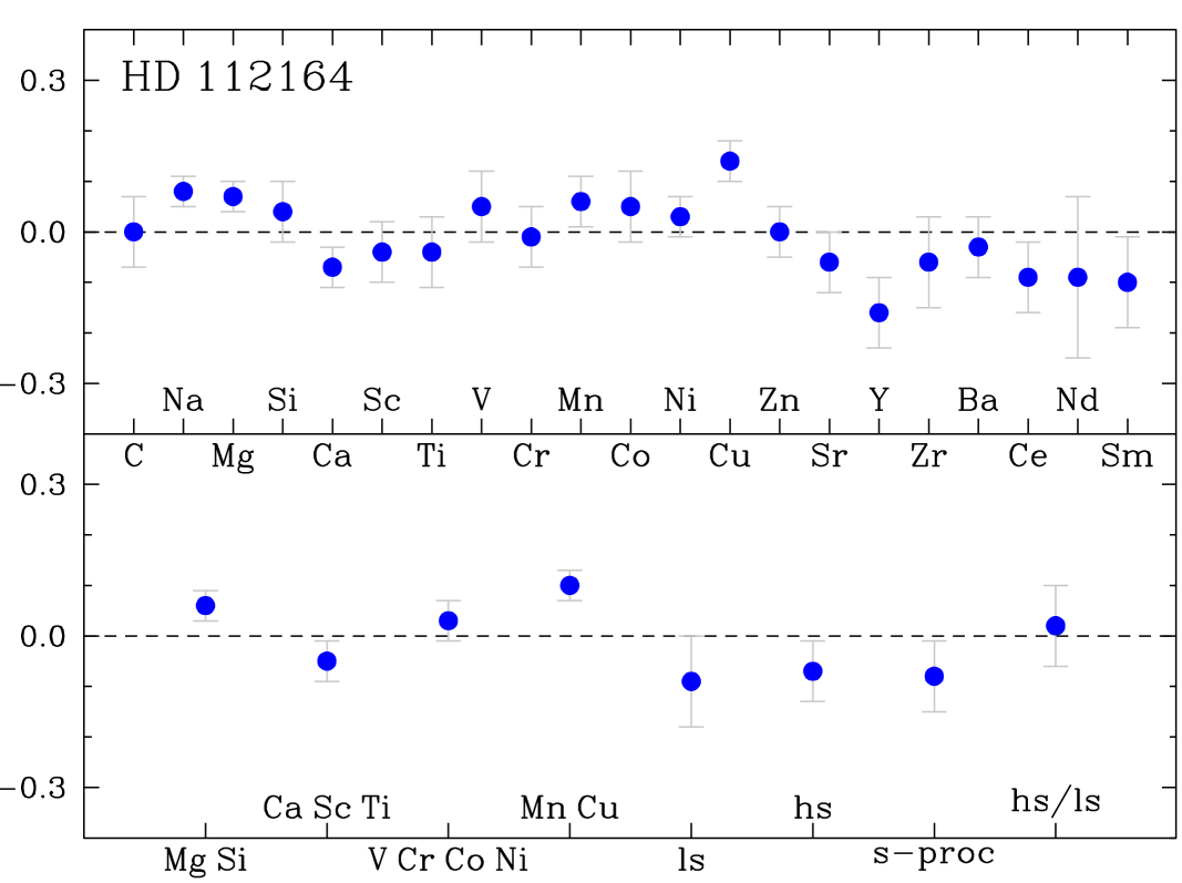
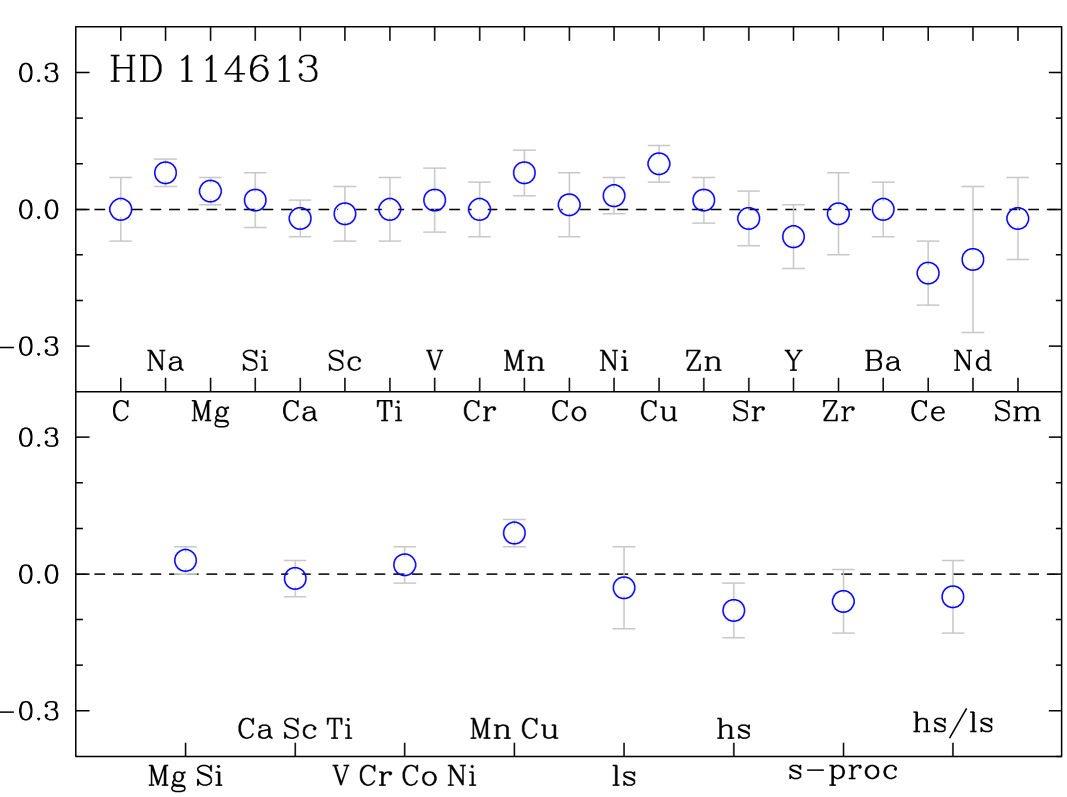
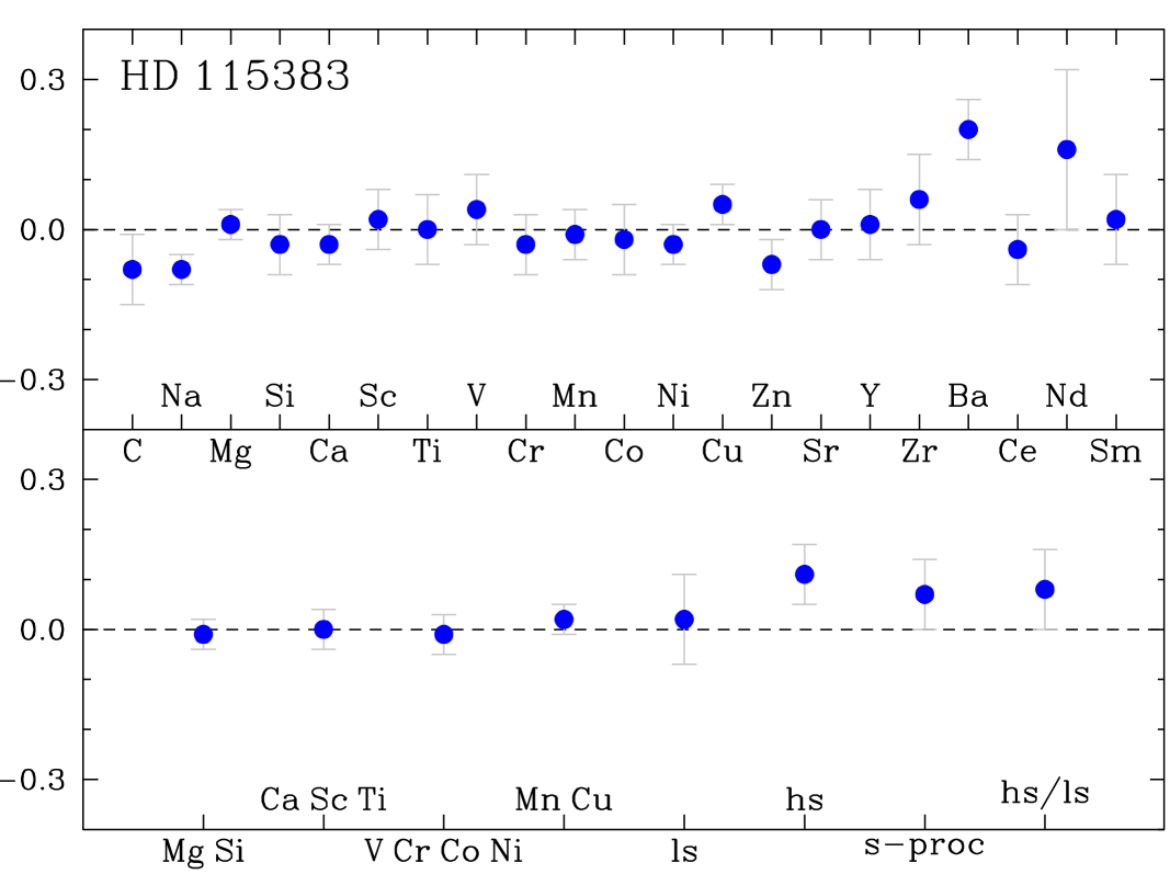
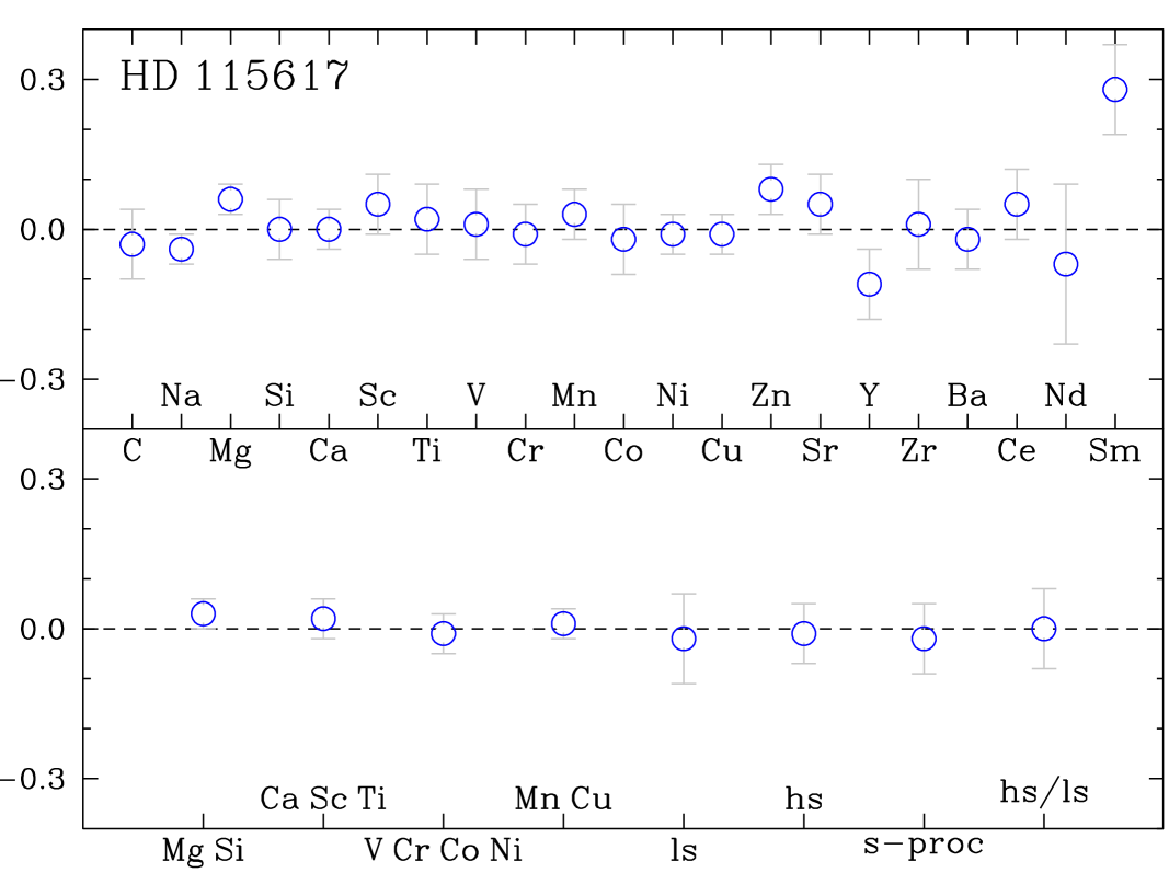
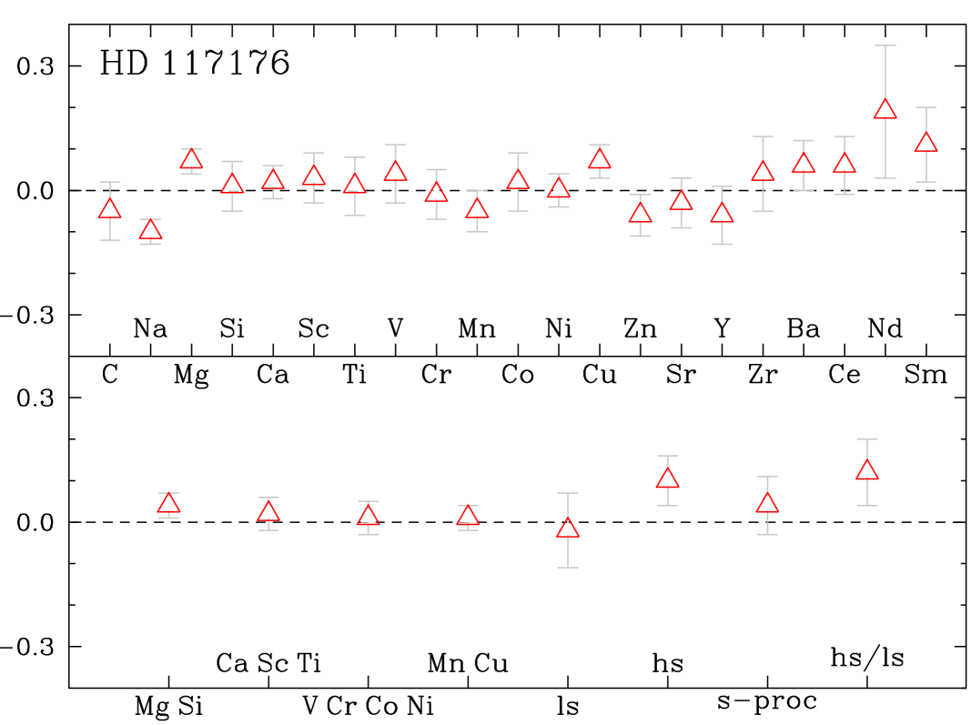
Figure 7: Abundance ratios [X/Fe] for individual elements (top of each panel) and $\langle$[X/Fe]$\rangle$ for the nucleosynthetic groups (bottom of each panel). The uncertainties adopted are those listed in Tables 3 and 7. The symbols represent the stellar classification defined in Sect. 5 (see Fig. 6).

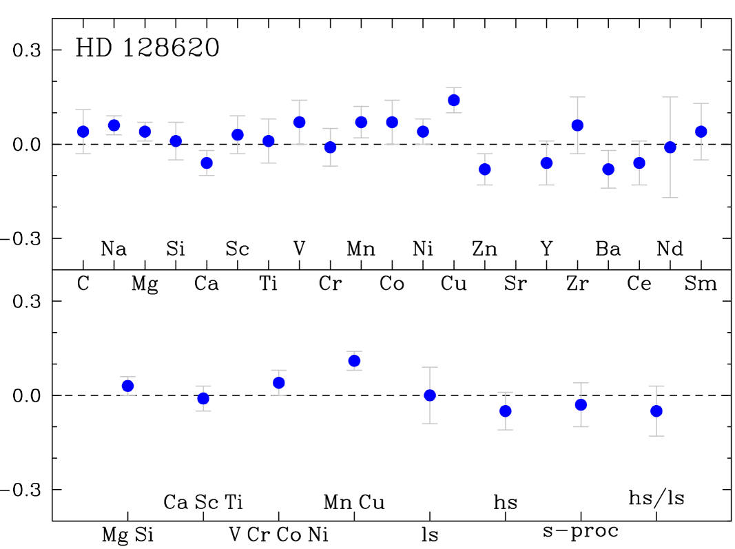
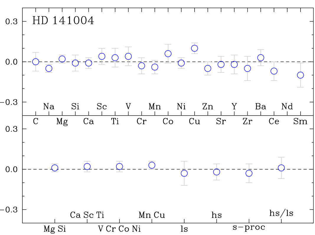
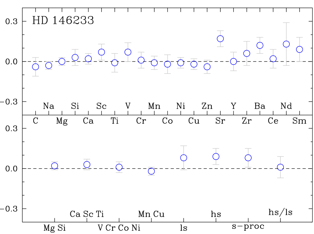
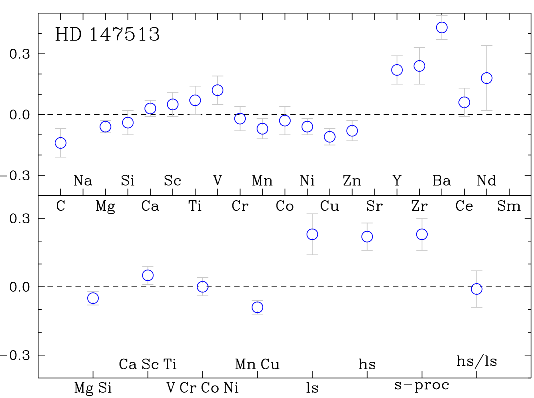
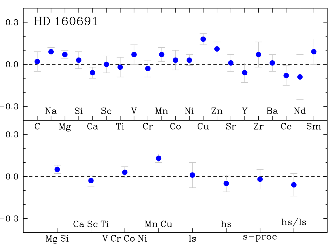
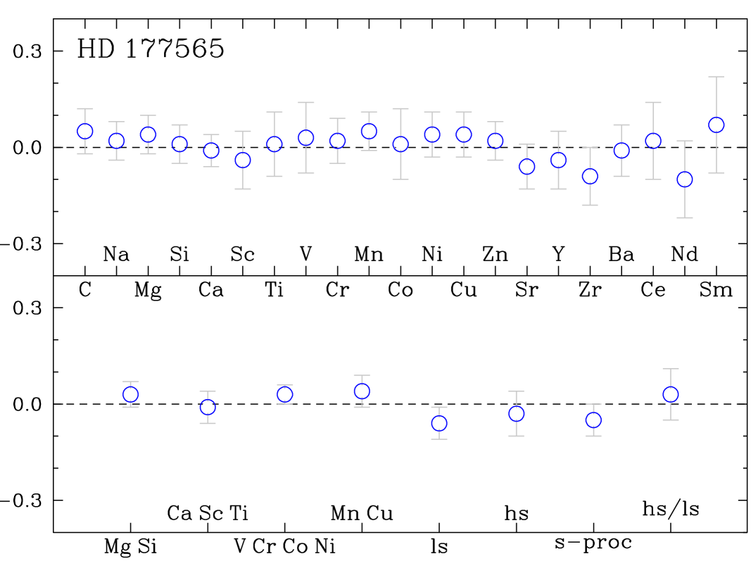
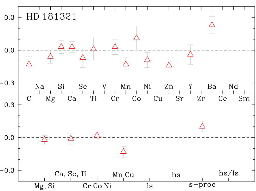
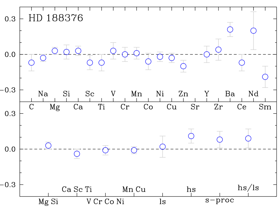
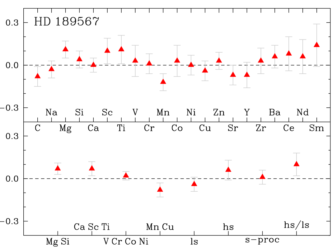
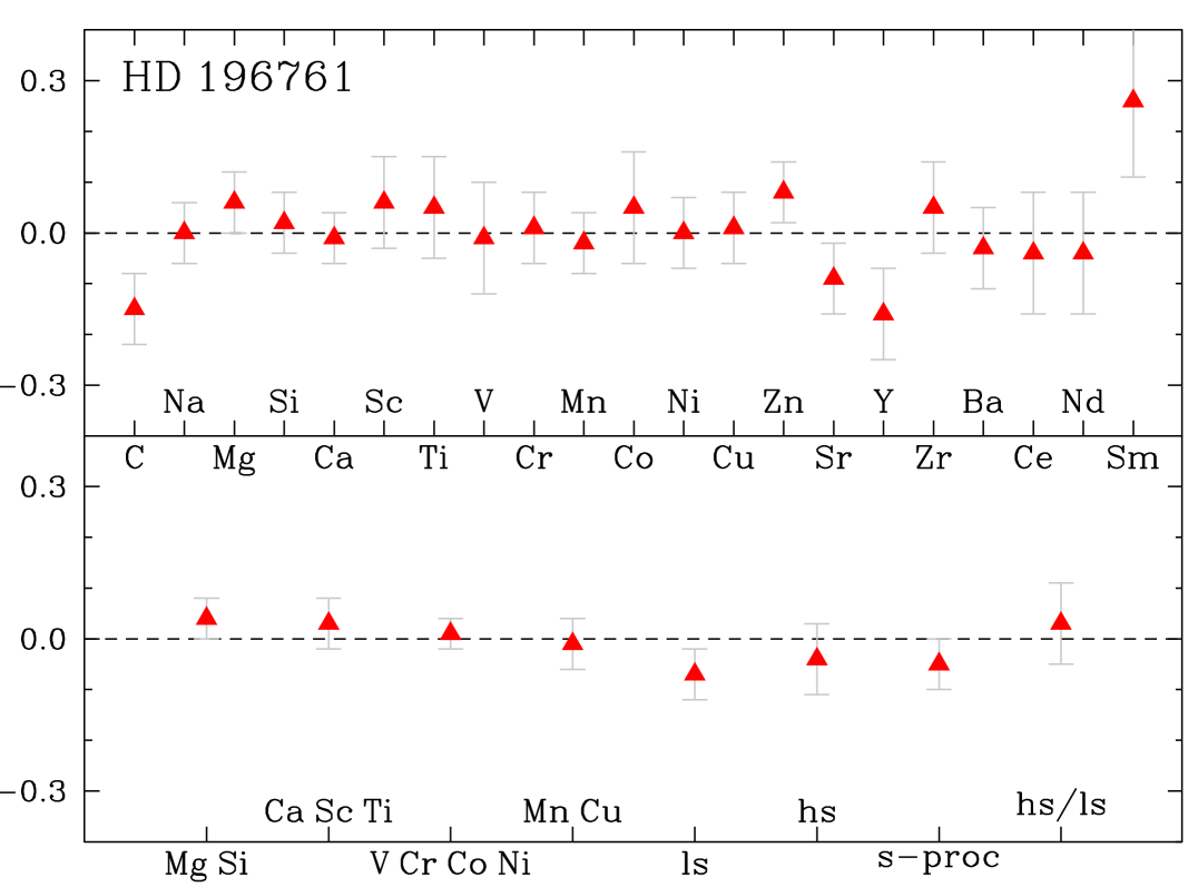
Figure 7: continued.

It is also very worthwhile to investigate the chemical abundances in stars that share similar values of age, metallicity, and Galactic orbit ($R_{\rm m}$ and $e$). These subgroup of stars are supposed to share the same physical conditions of the Galaxy at the time and galactocentric position of their birth. An example of this includes the stars HD 43834, HD 84117, HD 141004, and HD 146233, which also have ages, metallicities, and Galactic orbits close to the solar values (they were all classified as intermediate abundance stars in the tree clustering analysis, one in slight underabundance and the three others in slight overabundance with respect to the Sun). In spite of this, only HD 43834 and HD 141004 show solar abundances, within the uncertainties, for all (or almost all) elements. HD 84117 is deficient in Mn and enriched in Na and in elements of the s-process (Sr, Y, Zr, and Ba). HD 146233, proposed by Porto de Mello & da Silva (1997b) as the closest solar twin ever known at that time, is actually (as also proposed by these authors) enriched in some elements of the s-process (Sr and Ba) and possibly enriched in Sc, V, and Sm. Thus, possibly, the investigation of a larger sample of stars at a similar level of detail as done here could reveal that non-solar abundance ratios are present even for stars sharing the same place and time of birth. Whether this reflects intrinsic heterogeneities in their natal interstellar clouds (in principle a reasonable hypothesis since the elements reflecting non-solar ratios are related to different nucleosynthetic processes operating in different timescales) or else is evidence for considerable radial migration in the Galaxy is a question we plan to address in a subsequent work involving a larger sample.

Still concerning the relations involving the stellar groups from the clustering analysis and the kinematic and orbital parameters of our sample, we can see in Fig. 5 that the group of metal-poor and old stars seems to have larger velocities in the direction of the Galactic centre ($|$$U_{\rm LSR}$$|>$ 40 km s^-1) and larger eccentricities ($e\gtrsim 0.2$) than the other stars. The star HD 50806 appears to have a singular position in this figure (in particular, it has the most eccentric orbit among the sample stars), which is probably related to its membership in the transition population of thin-thick disc stars. The limitation of our sample does not allow to verify the results of Rocha-Pinto et al. (2006) that metal-poor and old stars show more orbital radial spread in the Galaxy.

6.2 Abundance trends as a function of [Fe/H]

Through the analysis of Fig. 8 we investigate possible trends in the abundance ratios as a function of the stellar metallicity. These trends are more clearly identified if the elements are grouped together, either based on their nucleosynthetic origin or because they share similar trends in the diagrams. For this reason, we show in the bottom panels of this figure the mean abundance $\langle$[X/Fe]$\rangle$ of a few groups of elements as a function of the metallicity (the same groups plotted in Fig. 7 and listed in Table 7). The stars are also identified according to the tree clustering analysis. We have fitted linear regressions on the diagrams in three ranges of metallicity: for stars poorer than the Sun, for stars of solar metallicity or richer, and for all the sample stars. We have then computed the cross-correlation coefficients in these three metallicity ranges and plotted the regressions of the more significant trends (only if $|\,r\,|\geq 0.5$).

Table 6: Carbon abundance ratios derived from the spectral synthesis of the two atomic lines ($\lambda$5052.2 and $\lambda$5380.3) and the two ${\rm C}_{2}$ band heads ($\lambda$5128 and $\lambda$5165) studied. Column 6 shows the final values adopted.

Star	[C/Fe] $\lambda 5052$		[C/Fe] $\lambda 5380$		[C/Fe] $\lambda 5128$		[C/Fe] $\lambda 5165$		[C/Fe]
HD 1835	0	.07	0	.05	0	.02	0	.04	0	.05
HD 20807	0	.06	0	.05	$-$0	.11	0	.05	0	.01
HD 26491	0	.01	0	.01	$-$0	.06	$-$0	.04	$-$0	.02
HD 33021	$-$0	.05	$-$0	.04	$-$0	.14	$-$0	.19	$-$0	.11
HD 39587	$-$0	.07	$-$0	.07	$-$0	.12	$-$0	.12	$-$0	.10
HD 43834	$-$0	.04	0	.01	0	.01	0	.02	0	.00
HD 50806	0	.21	0	.13	0	.08	0	.08	0	.13
HD 53705	$-$0	.07	$-$0	.04	$-$0	.14	$-$0	.07	$-$0	.08
HD 84117	0	.09	0	.07	$-$0	.06	$-$0	.06	0	.01
HD 102365	0	.07	0	.12	$-$0	.08	0	.02	0	.03
HD 112164	$-$0	.01	$-$0	.01	0	.00	0	.02	0	.00
HD 114613	$-$0	.01	$-$0	.02	0	.03	0	.00	0	.00
HD 115383	$-$0	.12	$-$0	.09	$-$0	.05	$-$0	.05	$-$0	.08
HD 115617	$-$0	.11	$-$0	.04	0	.00	0	.04	$-$0	.03
HD 117176	$-$0	.06	$-$0	.04	$-$0	.06	$-$0	.04	$-$0	.05
HD 128620	0	.01	0	.04	0	.03	0	.07	0	.04
HD 141004	$-$0	.03	$-$0	.03	0	.00	0	.07	0	.00
HD 146233	$-$0	.04	$-$0	.05	$-$0	.07	0	.01	$-$0	.04
HD 147513	$-$0	.15	$-$0	.11	$-$0	.18	$-$0	.10	$-$0	.14
HD 160691	0	.01	$-$0	.01	0	.02	0	.06	0	.02
HD 177565	0	.05	0	.10	0	.02	0	.03	0	.05
HD 181321	–		$-$0	.10	$-$0	.15	$-$0	.15	$-$0	.13
HD 188376	$-$0	.16	$-$0	.06	$-$0	.02	$-$0	.05	$-$0	.07
HD 189567	0	.00	$-$0	.05	$-$0	.15	$-$0	.10	$-$0	.08
HD 196761	–		$-$0	.13	$-$0	.20	$-$0	.13	$-$0	.15

The overall trend of our abundance ratios as a function of the stellar metallicity normally follows what has been suggested in the literature concerning the nucleosynthetic origin of the elements and their abundance evolution in time (Chen et al. 2000; Reddy et al. 2003; Bensby et al. 2005; Chen et al. 2008; Neves et al. 2009). The light metals Ca, Sc, and Ti are predominantly produced by Type II Supernovae (SN II) at the beginning of the enrichment history of the Galactic disc. On the other hand, iron and the iron-peak elements V, Cr, Co, and Ni are predominantly synthesised by Type Ia Supernovae (SN Ia) in longer time scales. Therefore, it is expected that the abundance ratio of these light metals with respect to iron progressively decrease from metal-poor to metal-rich stars, whereas the abundance ratio of iron-peak elements with respect to iron, all produced at the same rate, remains constant and close to zero in the whole range of metallicity. Indeed, this is exactly what is observed in Fig. 8 for [Ca, Sc, Ti/Fe] and [V, Cr, Co, Ni/Fe], to within our stated abundance uncertainties.

The light metals Mg and Si may not only be produced by SN II considering that [Mg, Si/Fe] flattens out for metallicities higher than $-$0.1 dex. The same behaviour was found by Chen et al. (2000) and Neves et al. (2009), who suggested that SN Ia is possibly contributing. The star HD 50806 is clearly enriched in Mg (and in other elements as well) according to Fig. 8, probably reflecting its membership to the thin-thick disc transition.

The situation of Mn, Cu, and Zn is somewhat more complex. The hypothesis of production in SN Ia still stands, but this is probably not the unique source. Allen & Porto de Mello (2011), in their study of s-process enriched stars, suggested that SN Ia is the main source of production of manganese, in opposition to the conclusions of Feltzing et al. (2007), who suggested that this element is mainly produced by SN II. Our results in Fig. 8, which show an increasing trend of [Mn/Fe] as a function of [Fe/H] (see also the bottom panel of Fig. 6, in which there is a sequential crescent ordination of $\langle$[X/Fe]$\rangle$ from the metal-poor clustering group to the metal-rich one), seem to support the idea of an extra nucleosynthetic source for the Mn yields. Such an increasing trend is also usually attributed to a metallicity dependence in the production of Mn in both SN Ia and SN II. In this work, Mn and Cu were plotted together through the mean abundance ratio [Mn, Cu/Fe]. Both these elements have abundances that increase with metallicity, though for Cu this trend is not as significant as for Mn, and seems to happen only for higher metallicities, being constant and close to zero for [Fe/H] $<$ 0. Cu and Zn, although being adjacent elements in the periodic table, stand in the transition between iron-peak and s-process elements, and their behaviour is in sharp contrast. A decreasing trend in [Zn/Fe] vs. [Fe/H] is seen for stars poorer than the Sun, in agreement with Fig. 1 of Allen & Porto de Mello (2011).

Table 7: Groups of chemical elements and uncertainties in the mean abundance ratios $\langle$[X/Fe]$\rangle$. The estimated errors are compared to the dispersions around the mean. For each group, the larger value of each observation run was adopted.

Nucleosynthetic group		HD 146233		HD 26491
		$\sigma_{\rm est}$	$\sigma_{\rm disp}$	$\sigma_{\rm est}$	$\sigma_{\rm disp}$
light metals	Mg, Si	0.03	0.02	0.04	0.03
light metals	Ca, Sc, Ti	0.03	0.04	0.05	0.01
iron peak	V, Cr, Co, Ni	0.03	0.04	0.02	0.03
iron peak	Mn, Cu	0.03	0.01	0.05	0.02
light s-process	Sr, Y, Zr	0.04	0.09	0.05	0.01
heavy s-process	Ba, Ce, Nd	0.06	0.06	0.06	0.07

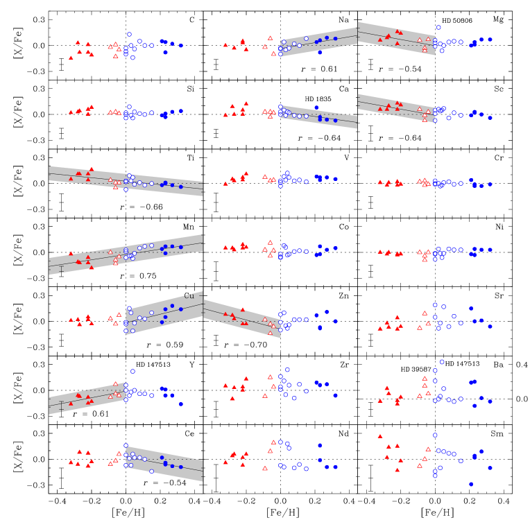
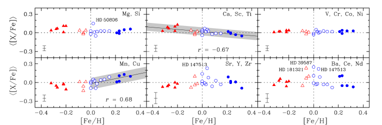
Figure 8: Abundance ratios as a function of the stellar metallicity for individual elements (top panels) and for nucleosynthetic groups (bottom panels). The ordinate axis has a different scale for [Ba/Fe] due to its larger abundances. The linear regressions (solid line), the 95% confidence intervals (hashed area), and the cross-correlation coefficients are also shown for $|\,r\,|\geq 0.5$. The symbols follow the classification of Sect. 5 (see Fig. 6).

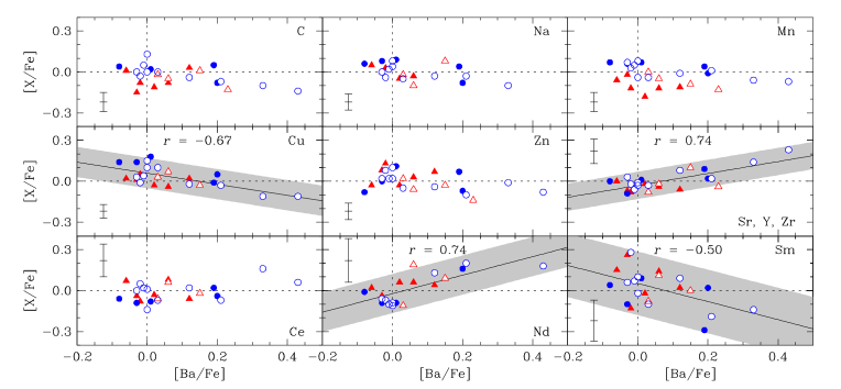
Figure 9: Abundance ratios as a function of [Ba/Fe]. For the elements of the light s-process (Sr, Y, and Zr) the mean abundance ratios are plotted. The linear regressions (solid line), the 95% confidence intervals (hashed area), and the cross-correlation coefficients are also shown for $|\,r\,|\geq 0.5$. The symbols follow the classification of Sect. 5 (see Fig. 6).

The elements C and Na were not grouped together with other elements. C is synthesised in several different sites and behaves similarly to O and N, with [C/Fe] decreasing with increasing metallicity. This negative trend is mostly observed in the metal-poor regime ([Fe/H] $<-$0.3), hence not seen in Fig. 8 given the limited metallicity range of our program stars. Nevertheless, our results agree very well with the recent C abundance determination performed by da Silva et al. (2011) for solar-like dwarfs. Na is probably produced, among other processes, in the core of massive stars and ejected by SN II into the interstellar medium. Here we found that [Na/Fe] is constant and nearly close to zero in the range of metal-poor stars, with a possible increasing trend for higher metallicities. Chen et al. (2000) suggested that maybe [Na/Fe] is close to zero for the whole metallicity range of disc stars. Neves et al. (2009), however, found that [Na/Fe] is close to zero for thin disc stars for [Fe/H] between $-$0.2 and +0.2, but above solar for other values of metallicity.

The [X/Fe] abundance ratios of elements of the s-process, mainly produced in TP-AGB of intermediate or low mass stars, and the r-process, produced in sites with high neutron density such as the final stages of massive stars (SN II, neutron stars), are supposed, respectively, to progressively increase and decrease from metal-poor stars to higher metallicities. These facts reflect the production of these elements in different time scales with respect to iron, the former products of long-lived AGB stars, the latter arising from short-lived massive stars which explode as supernovae. This is not clearly observed in the diagrams of Fig. 8 for Sm and the s-process elements because of the short metallicity range. An interesting result of the analysis of these diagrams are the properties involving some Ba-enriched stars, which we discuss in the next section.

6.3 Abundance trends as a function of [Ba/Fe]

A few stars in our sample are remarkably enriched in Ba by more than 3$\sigma$, especially HD 39587 and HD 147513. For this reason we also investigated the behaviour of the abundance ratios [X/Fe] or $\langle$[X/Fe]$\rangle$ as a function of [Ba/Fe] for some elements or groups of elements showing some kind of relation with the production of barium (see Fig. 9). Once more, we computed the cross-correlations coefficients and we plotted in the figure the regressions of the most significant trends ($|\,r\,|\geq 0.5$).

Castro et al. (1999) proposed the existence of an anticorrelation between the abundances of Cu and the s-process elements. They found that [Cu/Fe] decreases with the increasing of [Ba/Fe], suggesting a relation between the destruction of Cu and the production of Ba (and other s-process elements). In the recent analysis of Ba-enriched stars of Allen & Porto de Mello (2011), the authors have not supported this scenario, arguing that Cu seems to be little (or not at all) affected by the s-process, even though they have acknowledged that some Ba-rich stars do present anticorrelated abundances of Cu and the s-process elements. Our results point to a statistically significant decrease in the abundances of Cu with increasing [Ba/Fe], in accordance with Castro et al. (1999).

Two other iron-peak elements, Mn and Zn, are also shown in Fig. 9 and no clear correlation is observed. This may indicate that Mn and Cu do not share the same nucleosynthetic origin. Indeed, Allen & Porto de Mello (2011) found that the synthesis of Cu receives a larger contribution from not so massive stars than Zn, a result roughly in line with those of Castro et al. (1999) and ours. Such results point towards the necessity of both more extensive observations of the abundances of Cu and Zn, and more protracted theoretical efforts, in order that a better understanding of the complex chemical history of these two elements may be achieved.

Castro et al. (1999) also proposed an anticorrelation in the abundances of C and Na with respect to [Ba/Fe]. Our results do not seem to support this anticorrelation, though our most Ba-rich stars, the Ursa Major group members HD39587 and HD147513, are markedly C-deficient. Porto de Mello & da Silva (1997a) attributed the [C/Fe] deficiency of a barium star to the ${}^{13}{\rm C}(\alpha,n)^{16}{\rm O}$ reaction that occurred in the hot-bottom envelope of its companion during the TP-AGB phase. However, HD39587 and HD147513 are no longer regarded as true barium stars.

Figure 9 shows an evident expected correlation for the light s-process elements (Sr, Y, and Zr). Correlations involving Nd, another heavy element of the s-process may also exist, but its abundance determination has larger uncertainties. An anticorrelation between [Sm/Fe] and [Ba/Fe] also seems to exist. Sm is a good representative of the r-process elements, and despite the very large uncertainties in the determination of such elements, usually showing very few lines in the spectra of solar-type stars, an interpretation in which this anticorrelation is due to ever more efficient production of s-process elements in AGB stars, as compared to the production of the r-process in SN II, seems warranted.

6.4 Abundance trends as a function of age

One of the motivations of the present paper is to explore the abundance ratios of elements due to different nucleosynthetic processes and the stellar ages, taking advantage of the reasonably precise ages that can be attributed to our program stars. Figure 10 shows the diagrams [X/Fe] and $\langle$[X/Fe]$\rangle$ as a function of the stellar age, and Fig. 11 explores the relation between the abundance ratios [X₁/X₂] of different elements and age. Similarly to Fig. 8, we have fitted linear regressions on the diagrams in three ranges of stellar age: for stars younger than the Sun ($age<$ 4.53 Gyr), for stars older than the Sun, and for all the sample stars. We have then computed the cross-correlation coefficients in these three ranges of stellar age and plotted the regressions of the more significant trends (only if $|\,r\,|\geq 0.5$). In these figures there are positive, negative, or flat abundance trends in the three ranges of age. We notice, however, that the age of the Sun, used as a reference, was arbitrarily chosen. The exact value of the transition age when the abundance behaviour changes is not clear from these plots (it is a value between 4 and 6 Gyr).

In spite of the long recognition (though not undisputed) of the so-called age-metallicity relation (see Fig. 12), the individual abundances in Fig. 10 and those in Fig. 8 do not share exactly the same behaviour, leading us to suggest in the following that the age-metallicity relation may be a multidimensional concept. For this reason, we regrouped the elements according to their abundance behaviour with age (see the bottom panels of Fig. 10).

Carbon and sodium do not seem to present any important trends of [X/Fe] with age. The positive trends observed for Mg, Sc, and Ti (less clearly seen for Si and Ca) are simply the result of the Galactic chemical evolution. The production rate of these elements by SN II decrease with time since the formation of the Galactic disc (equivalently to increasing with age) compared to the increased production of Fe by the longer-lived SN Ia as we approach more recent epochs. Silicon perhaps shows no trend at all; Mg seems to have a more or less positive linear trend with increasing age; in their turn Ca, Sc, and Ti sport a more complex behaviour. The statistical significance of the behaviour of Ca is slight, and not much confidence should be placed in the apparent [Ca/Fe] decrease with time, followed by an increase towards more recent times. Taken at face value, this would appear to lend support to the suggestion that some fraction of the Ca synthesis might be due to SN Ia, in unison with their production of Fe. Sc and Ti seem to have a significant decrease with time with respect to Fe, but this decrease stops at a time close to the solar age and flattens thereafter towards present times.

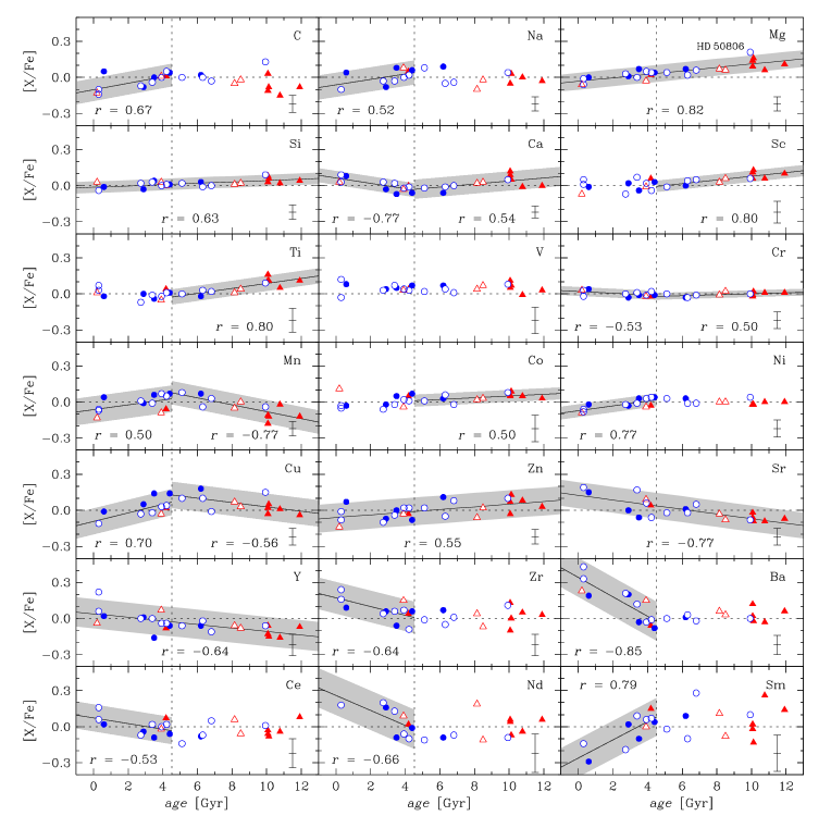
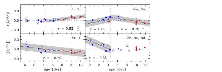
Figure 10: Abundance ratios as a function of the stellar age for individual elements (top panels) and for nucleosynthetic groups (bottom panels). The vertical dashed line indicates the adopted solar age (4.53 Gyr). The linear regressions (solid line), the 95% confidence intervals (hashed area), and the cross-correlation coefficients are also shown for $|\,r\,|\geq 0.5$. The symbols follow the classification of Sect. 5 (see Fig. 6).

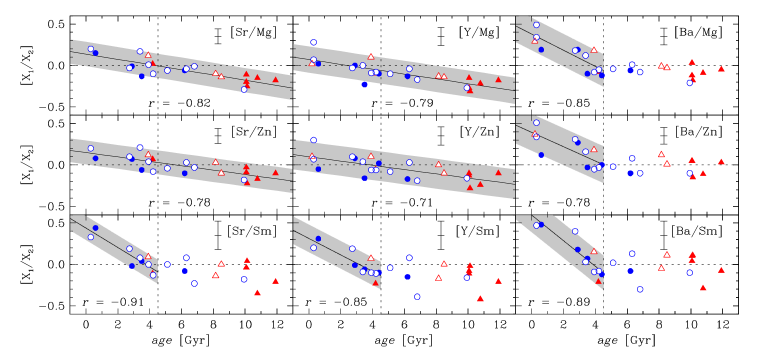
Figure 11: Abundance ratios as a function of the stellar age. The vertical dashed line indicates the adopted solar age (4.53 Gyr). The linear regressions (solid line), the 95% confidence intervals (hashed area), and the cross-correlation coefficients are also shown for $|\,r\,|\geq 0.5$. The symbols follow the classification of Sect. 5 (see Fig. 6).

Among the Fe-peak elements, no important trend is seen in the [X/Fe] relation with age for V, Cr, Co, and Zn; only a dubious one for Ni in the interval of young stars. Yet, again, Cu and Mn suggest more underlying complexity. Even though the statistical significance of the linear regressions is slight, the abundance ratios to Fe of both these elements seem first to increase towards the present epoch, and then decrease (a behaviour that is reinforced when these two elements are plotted together through the mean abundance ratio [Mn, Cu/Fe]). Recalling that Allen & Porto de Mello (2011) have found that Mn is mostly due to SN Ia, our result could imply that the relative yield of Mn to Fe in SN Ia decreases with time (and consequently the overall metallicity). The situation for Cu is less straightforward, as usual. Allen & Porto de Mello (2011) suggest that little of the synthesis of Mn, Cu, and Zn is owed to the main s-process, leaving the action of AGB stars an unlikely source of such a behaviour. These same authors assert that the action of the so-called weak s-process, sited at the He-burning core of massive stars, has a non negligible contribution to the synthesis of Mn, Cu, and Zn. One possible explanation for the decrease of the abundance ratios of [Mn/Fe] and [Cu/Fe] towards more recent times is a decreasing yield of the weak s-process in their synthesis, as contrasted to the production of Fe by SN Ia. Clearly, an understanding of the detailed chemical evolution of elements, in both the dimensions of metallicity and age, of the Fe-peak and its transition with the heavier elements deserves closer scrutiny, both observationally and theoretically.

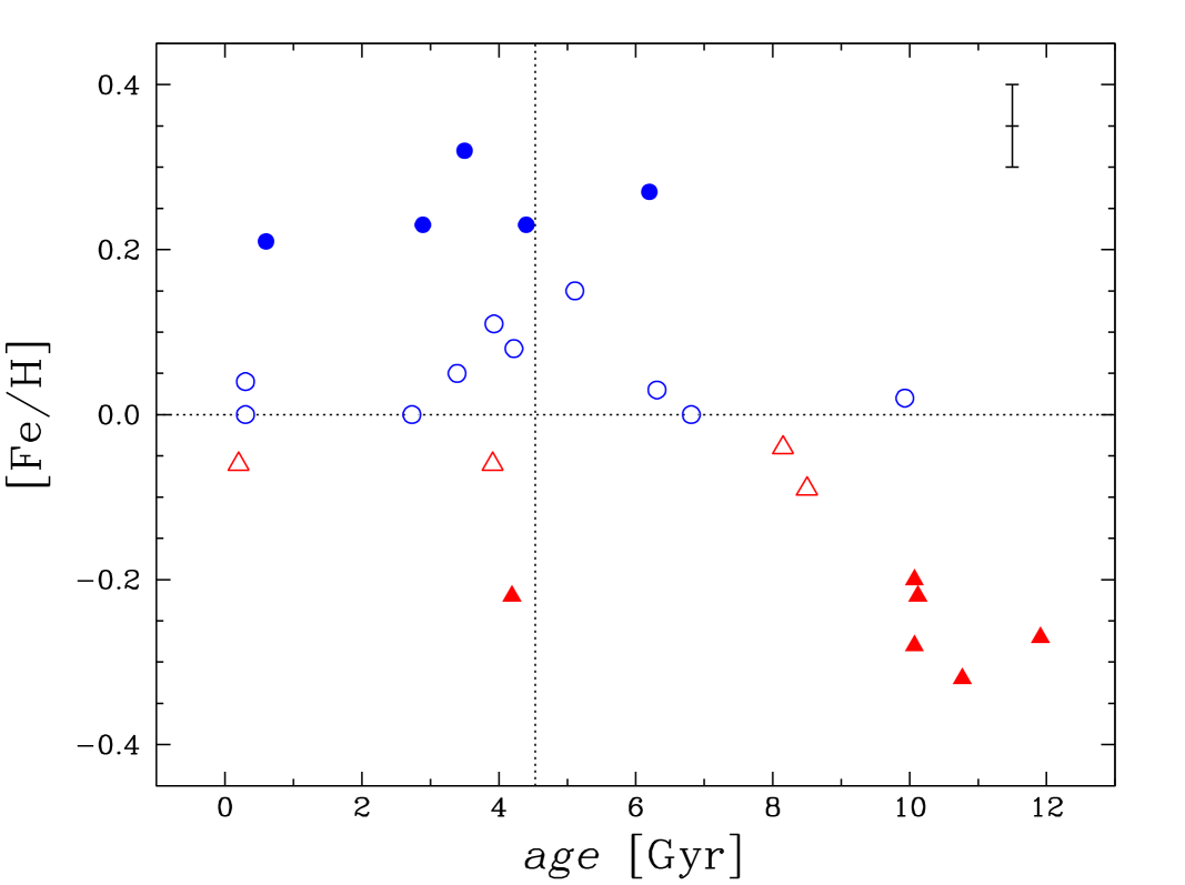
Figure 12: Stellar metallicity as a function of age. The symbols follow the classification of Sect. 5 (see Fig. 6).

We next turn to the [X/Fe]-age relation for the s-process elements. These present particular interest, since Castro et al. (1999) suggested, also using data from Edvardsson et al. (1993), that [Ba/H] has a steeper decrease with age than [Fe/H], and therefore that [Ba/Fe] increases towards modern times (see also Bensby et al. 2007). This fact might be interpreted, again, as a consequence of the larger yield of the s-process element synthesis by the long-lived AGB stars in relation to the not as-long-lived production of Fe by SN Ia. Do the other s-process elements show a behaviour similar to barium? Apparently this is so, but not in a straightforward way. The lighter s-process elements Sr and Y seem to have a linear trend of [X/Fe] with age (clearly seen for Sr), increasing towards present times, as expected. The [Zr/Fe], [Ce/Fe], and [Nd/Fe] ratio, however, appears flat in the old age regime, possibly increasing only for stars younger than the Sun. The [Ba/Fe] ratio behaves similarly but the increase towards younger ages is much sharper and more significant. At face value, these results point towards the evolution of the relative yields of such s-process elements with time (and metallicity) in AGB stars, apparently favouring the heavier species Ba and Nd over lighter ones. The simultaneous analysis of the [Cu/Fe] and [s-process/Fe] ratios, epitomised, for example, by the [Ba/Fe] relation with age, suggests an anticorrelation of Cu and Ba towards younger stars, as found by Castro et al. (1999), adding to the controversy surrounding the chemical evolution of copper.

Finally, a positive trend with increasing age is observed for [Sm/Fe] in stars younger than the Sun, again reflecting the smaller number of SN II than SN Ia in the present in comparison with the past (in this case the epoch of the Sun’s formation). Significant positive trends are also observed for Ni and Cu in the regime of younger stars.

Concerning the four groups yielded by the tree clustering analysis and their relation with age, we can only state that, as expected, the old stars in our sample are also metal-poor, whereas young stars tend to be metal-rich. Once more, the case of the star HD 50806 is evidenced. Although classified in the intermediate group of stars with slightly over-solar abundances ($\langle$[X/H]$\rangle$ = +0.06 dex), it is situated close to the group of metal-poor stars ($\langle$[X/H]$\rangle$ = $-$0.24 dex) in Fig. 10, which is maybe a consequence of its population membership.

The bottom panels of Fig. 10 shows the average of the [X/Fe] relations with age for selected groups of elements. Thus we see that grouping Sc and Ti reinforces the relation with age already shown by each element individually, and the same is seen for the grouping of Sr and Y. Similarly, averaging the [X/Fe] relations with age for Zr, Ba, and Nd produces a very steep increase towards present epochs, after a flat relation from the birth of the Galactic disc up to the solar age.

These results prompted us to investigate the specifics of the [X₁/X₂] ratios with age, where X₁ and X₂ designate elements other than Fe. In Fig. 11 we explore the time evolution of some elements that displayed a particular clear [X/Fe] relation with age. Thus, it is apparent that the [Ba/Mg] and [Ba/Zn] increase steeply towards present epochs, for stars younger than the Sun, reinforcing their individual and opposite behaviour in the [X/Fe]-age diagrams. Also, both [Sr/Mg] and [Y/Mg] increase linearly and significantly from the oldest to the youngest stars; the same is seen in the [Sr/Zn] and [Y/Zn] ratios. Investigating the [X₁/X₂] ratios of s-process to r-process elements, we found steep increases in the [Ba/Sm], [Sr/Sm], and [Y/Sm] ratios towards younger stars, but only for objects younger than the Sun. Significant age relations are, therefore, evidenced in the [X₁/X₂] ratios of diverse elements, representing a wide range of nucleosynthetic processes and tentatively allowing the proposition that the age-metallicity relation is a more complex constraint to Galactic chemo-dynamical models than hitherto recognised.

6.5 Abundance trends with condensation temperature

Our determination of multi-elemental abundances also provides the study of possible trends in the abundance ratios [X/Fe] as a function of the condensation temperature ($T_{\rm C}$) of each element. Values of 50% $T_{\rm C}$  (the temperature when 50% of an element is in the condensed phase) for a solar-system composition gas were taken from Lodders (2003) and Lodders et al. (2009).

For a few stars in our sample we have found some correlations of [X/Fe] with $T_{\rm C}$  (even after corrections due to Galactic chemical evolution effects were applied). However, no clear correlation seems to exist when comparing the slopes for refractory elements (those with $T_{\rm C}$ $\gtrsim$ 900 K) with several stellar parameters ($T^{\rm mean}_{\rm eff}$, [Fe/H], $\log{g}$, $\xi$, mass, and age). The one involving the metallicity was proposed by Ramirez et al. (2010) in the sense that higher-metallicity stars present more negative slopes. Our results agree with their paper, but the number of metal-rich stars in our sample is too small to confirm their conclusions.

7 Conclusions

In this work we have performed a multi-elemental, differentially with respect to the Sun, spectroscopic analysis of a sample of 25 solar-type stars in the solar neighbourhood. We have derived their atmospheric parameters (from various nearly independent criteria and with low internal errors), masses, ages, kinematical and orbital parameters, and elemental abundances (derived with very low internal uncertainties) based on equivalent widths or spectral synthesis.

Despite small in size, our sample was carefully selected to undergo an homogeneous and detailed analysis based on spectra with high resolution and high signal-to-noise ratio. We have: (i) checked the effective temperatures based on the excitation equilibrium of neutral iron lines against those from photometric calibrations and from the H$\alpha$ wings profile, (ii) checked the surface gravities computed through the ionisation equilibrium between Fe I and Fe II lines against those computed based on the evolutionary parameters, (iii) derived masses and ages from evolutionary tracks and isochrones computed considering the metallicity of each star, and (iv) applied a differential spectroscopic analysis relative to the Sun, hence minimising the systematic errors and yielding a mean uncertainty of 0.06 dex in the abundance ratios. We thus expect that our determinations have achieved a high level of precision and accuracy.

We have also applied a statistical study to our abundance results using the method of tree clustering analysis, through which we looked for groupings of stars that share similar abundances in the [X/H] space. Although our sample has a limited range in metallicity, it covers a broad range in age. The detailed abundance pattern was then investigated through correlations with kinematics, Galactic orbits, and stellar ages. Our conclusions are thus summarised:

• Four groups were identified, two having over-solar abundances (with averages +0.26 and +0.06 dex on [X/H]), and two with under-solar abundance values (on average $-$0.06 and $-$0.24 dex). Possible non-solar abundance ratios, even for stars which share the same age, Galactic orbit, and metallicity as the Sun, are suggested. Whether these are due to heterogeneity in the stellar natal clouds, or by dynamical migration within the Galactic disc, should be investigated with larger samples. In particular, the results of Rocha-Pinto et al. (2006) that metal-poor and old stars show more orbital radial spread in the Galaxy could not be verified given the limitation of our sample;

• The presence of Ba-enriched stars in our sample prompted us to investigate in detail the relation of some elements with Ba. An anticorrelation between [Cu/Fe] and [Ba/Fe] was found, in line with similar claims in the literature. The [Sm/Fe] abundance ratios seem to be anticorrelated with [Ba/Fe], barely at the 95% confidence level. On the other hand, previous suggestions of [C/Fe] and [Na/Fe] anticorrelations with [Ba/Fe] could not be confirmed. Even though the possible connected chemical evolution of Mn, Cu, and Zn has been recently discussed in the literature, no significant trend of [Mn/Fe] and [Zn/Fe] with [Ba/Fe] is suggested;

• The consideration of the [X/Fe] ratios with age revealed much differing behaviour of the elements, suggesting that the age-metallicity relation has more underlying complexity than commonly recognised. The [Mg/Fe], [Sc/Fe], and [Ti/Fe] decrease towards younger ages. The [Cu/Fe] and [Mn/Fe] ratios initially increase towards younger stars up to the solar age, and then decrease towards the youngest objects, a result that may speak of differing yields in the SN Ia production of these elements, related to metallicity and age, as well as a possible influence of the evolution with time of the weak s-process yields, operating off of massive stars. The steepest relation with age was found for the [Ba/Fe] ratio, but only for ages younger than the solar one, and a similar but less evident behaviour is seen for Zr, Ce, and Nd. Other heavy s-process elements, however, such as Sr and Y, show a linearly increasing [X/Fe] towards younger ages, particularly clearer for Sr. [Sm/Fe] significantly decreases for stars younger than the Sun. Thus, the [Cu/Ba] ratio clearly decreases towards younger stars, and the same is seen at a significant level for [Sm/Ba];

• Considering the average of elements with similar behaviour with age considerably reinforces the aforementioned results, particularly for the [Sc,Ti/Fe], [Mn,Cu/Fe], [Sr,Y/Fe], and [Zr,Ba,Nd/Fe] relations;

• The consideration of element ratios not directly involving Fe shows some marked behaviour. Particularly, the [Ba/Mg], [Ba/Zn], [Ba/Sm], [Sr/Sm], and [Y/Sm] steeply increase towards younger ages for stars younger than the Sun. Also, the [Sr/Mg] and [Y/Mg] ratios linearly increase towards younger ages, and the same is seen for [Sr/Zn] and [Y/Zn];

• Possible correlations of the abundances, the condensation temperatures of the different elements, and the presence of exoplanets in our program stars was deeply investigated, but no significant correlation was found.

The detailed consideration of precise element abundances derived from high-quality atmospheric parameters and spectroscopic data, tied to masses, kinematics, and ages for solar-type stars, generally provides a wealth of interesting data, contributing towards a broader understanding of the evolution of the Galaxy in its chemical and dynamical aspects.

Table 8: Atomic line parameters of the elements used in the analysis. Oscillator strengths ($\log{gf}$) and raw $EW$s (before the conversion set out by Eq. 1 and  2), given in mÅ, of both the Ganymede spectra observed in the first (Gany 1) and second (Gany 2) runs are listed (except for C, for which the analysis is based on spectral synthesis). Lines with missing $gf$ values represent the elements with hyperfine structure (Mg, Sc, V, Mn, Co, and Cu) and the detailed line splitting is shown in Table 9.

$\lambda$ [Å]	Id.	$\chi$ [eV]	Gany 1				Gany 2				$\lambda$ [Å]	Id.	$\chi$ [eV]	Gany 1				Gany 2
			$\log{gf}$		$EW$		$\log{gf}$		$EW$					$\log{gf}$		$EW$		$\log{gf}$		$EW$
5052.167	C I	7.68	$-$1	.48		–	$-$1	.62		–	4926.147	Ti I	0.82		–		–	$-$2	.17	7	.0
5380.322	C I	7.68	$-$1	.78		–	$-$1	.84		–	5022.871	Ti I	0.83	$-$0	.52	77	.3	$-$0	.35	79	.2
6154.230	Na I	2.10	$-$1	.52	42	.3	$-$1	.52	40	.8	5024.842	Ti I	0.82	$-$0	.66	71	.5	$-$0	.48	73	.8
6160.753	Na I	2.10	$-$1	.23	61	.8	$-$1	.29	59	.9	5071.472	Ti I	1.46		–		–	$-$0	.77	31	.3
4571.102	Mg I	0.00		–	107	.8		–	110	.3	5113.448	Ti I	1.44	$-$0	.86	30	.3	$-$0	.88	27	.6
4730.038	Mg I	4.34		–	78	.2		–	70	.9	5145.464	Ti I	1.46	$-$0	.67	38	.8	$-$0	.64	37	.6
5711.095	Mg I	4.34		–	119	.2		–	106	.4	5147.479	Ti I	0.00		–		–	$-$1	.98	42	.4
5785.285	Mg I	5.11	$-$1	.87	50	.5	$-$1	.82	55	.3	5152.185	Ti I	0.02		–		–	$-$2	.03	39	.1
5517.533	Si I	5.08	$-$2	.42	15	.7	$-$2	.51	13	.0	5192.969	Ti I	0.02	$-$1	.10	88	.3	$-$1	.02	84	.4
5621.607	Si I	5.08		–		–	$-$2	.61	10	.5	5211.206	Ti I	0.84	$-$2	.10	9	.1	$-$2	.07	9	.2
5665.563	Si I	4.92	$-$1	.98	42	.2	$-$1	.96	41	.8	5219.700	Ti I	0.02	$-$2	.32	27	.9	$-$2	.23	30	.0
5684.484	Si I	4.95		–		–	$-$1	.60	62	.3	5295.780	Ti I	1.07		–		–	$-$1	.60	13	.2
5690.433	Si I	4.93	$-$1	.80	52	.9	$-$1	.81	50	.6	5426.236	Ti I	0.02		–		–	$-$2	.97	7	.8
5701.108	Si I	4.93	$-$1	.90	46	.3	$-$1	.97	41	.0	5471.197	Ti I	1.44		–		–	$-$1	.48	9	.6
5708.405	Si I	4.95		–		–	$-$1	.35	79	.1	5490.150	Ti I	1.46		–		–	$-$1	.00	22	.6
5753.622	Si I	5.61		–		–	$-$1	.24	50	.8	5648.567	Ti I	2.49	$-$0	.40	11	.5	$-$0	.39	11	.1
5772.149	Si I	5.08		–		–	$-$1	.56	57	.7	5679.937	Ti I	2.47	$-$0	.65	6	.9	$-$0	.63	7	.0
5793.080	Si I	4.93	$-$1	.91	46	.0	$-$1	.94	42	.6	5739.464	Ti I	2.25	$-$0	.67	10	.5	$-$0	.75	8	.6
6125.021	Si I	5.61		–		–	$-$1	.50	34	.1	5866.452	Ti I	1.07		–		–	$-$0	.82	49	.6
6131.577	Si I	5.61	$-$1	.67	25	.8	$-$1	.65	26	.6	6064.629	Ti I	1.05		–		–	$-$1	.88	9	.7
6131.858	Si I	5.61	$-$1	.66	26	.6	$-$1	.64	27	.0	6091.177	Ti I	2.27		–		–	$-$0	.44	15	.9
6142.494	Si I	5.62	$-$1	.44	37	.5	$-$1	.45	36	.3	6092.798	Ti I	1.89	$-$1	.31	6	.0	$-$1	.28	6	.1
6145.020	Si I	5.61	$-$1	.40	40	.8	$-$1	.36	41	.8	6098.694	Ti I	3.06		–		–	$-$0	.16	6	.1
6243.823	Si I	5.61	$-$1	.22	52	.5	$-$1	.19	52	.7	6126.224	Ti I	1.07		–		–	$-$1	.40	23	.5
6244.476	Si I	5.61	$-$1	.26	49	.5	$-$1	.25	48	.6	6258.104	Ti I	1.44	$-$1	.46	54	.6	$-$0	.43	52	.3
5261.708	Ca I	2.52		–		–	$-$0	.65	99	.4	4568.345	Ti II	1.22	$-$2	.85	33	.6	$-$2	.85	32	.3
5581.979	Ca I	2.52		–		–	$-$0	.68	97	.2	4583.415	Ti II	1.16	$-$2	.85	36	.2	$-$2	.84	35	.1
5590.126	Ca I	2.52	$-$0	.78	96	.3	$-$0	.73	93	.9	4657.209	Ti II	1.24		–		–	$-$2	.31	55	.8
5867.572	Ca I	2.93	$-$1	.62	25	.3	$-$1	.59	25	.1	4798.539	Ti II	1.08	$-$2	.75	45	.4	$-$2	.70	44	.7
6161.295	Ca I	2.52	$-$1	.18	71	.6	$-$1	.08	69	.7	5211.544	Ti II	2.59	$-$1	.59	32	.1	$-$1	.54	33	.2
6163.754	Ca I	2.52		–		–	$-$1	.25	83	.4	5336.783	Ti II	1.58	$-$1	.77	71	.5	$-$1	.63	73	.4
6166.440	Ca I	2.52	$-$1	.18	71	.5	$-$1	.02	76	.9	5381.020	Ti II	1.57	$-$1	.91	65	.1	$-$1	.95	59	.5
6169.044	Ca I	2.52	$-$0	.75	99	.4	$-$0	.70	97	.0	5418.756	Ti II	1.58	$-$2	.21	49	.7	$-$2	.17	49	.4
6169.564	Ca I	2.52	$-$0	.51	117	.6	$-$0	.53	119	.8	5657.436	V I	1.06		–		–		–	9	.4
6449.820	Ca I	2.52		–		–	$-$0	.32	127	.8	5668.362	V I	1.08		–	8	.7		–	6	.7
6455.605	Ca I	2.52		–		–	$-$1	.43	53	.7	5670.851	V I	1.08		–	21	.1		–	21	.7
6471.688	Ca I	2.52		–		–	$-$0	.64	101	.5	5727.661	V I	1.05		–	10	.9		–	12	.5
6499.654	Ca I	2.52		–		–	$-$0	.86	87	.2	6090.216	V I	1.08		–	35	.6		–	34	.4
4743.817	Sc I	1.45		–		–		–	8	.5	6135.370	V I	1.05		–	12	.6		–	11	.5
5356.091	Sc I	1.86		–		–		–	1	.8	6150.154	V I	0.30		–	12	.6		–	11	.0
5392.075	Sc I	1.99		–		–		–	7	.0	6199.186	V I	0.29		–	15	.1		–	14	.0
5484.611	Sc I	1.85		–		–		–	3	.2	6216.358	V I	0.28		–		–		–	37	.0
5671.826	Sc I	1.45		–		–		–	19	.3	6274.658	V I	0.27		–		–		–	8	.7
6239.408	Sc I	0.00		–		–		–	9	.0	6285.165	V I	0.28		–	10	.4		–	16	.2
5318.346	Sc II	1.36		–		–		–	18	.2	4575.092	Cr I	3.37		–		–	$-$0	.88	13	.6
5357.190	Sc II	1.51		–	5	.4		–	5	.2	4616.120	Cr I	0.98		–		–	$-$1	.31	91	.9
5526.815	Sc II	1.77		–	77	.9		–	77	.6	4626.174	Cr I	0.97		–		–	$-$1	.47	84	.8
5657.874	Sc II	1.51		–	69	.8		–	69	.2	4708.019	Cr I	3.17		–		–	$-$0	.06	58	.1
5684.189	Sc II	1.51		–	40	.8		–	41	.2	4737.355	Cr I	3.09		–		–	$-$0	.06	62	.0
6245.660	Sc II	1.51		–	38	.0		–	35	.6	4756.137	Cr I	3.10	0	.09	74	.6	0	.03	66	.4
6320.867	Sc II	1.50		–	9	.1		–	8	.4	4801.047	Cr I	3.12	$-$0	.28	51	.5	$-$0	.28	46	.2
4518.023	Ti I	0.83	$-$0	.49	76	.2		–		–	4936.335	Cr I	3.11	$-$0	.35	48	.5	$-$0	.32	47	.2
4548.765	Ti I	0.83	$-$0	.55	73	.7		–		–	4964.916	Cr I	0.94		–		–	$-$2	.50	41	.6
4562.625	Ti I	0.02		–		–	$-$2	.73	11	.7	5200.207	Cr I	3.38	$-$0	.58	24	.6	$-$0	.50	26	.8
4617.254	Ti I	1.75		–		–	0	.23	64	.6	5214.144	Cr I	3.37	$-$0	.77	17	.7	$-$0	.73	18	.4
4758.120	Ti I	2.25	0	.44	56	.0	0	.26	43	.3	5238.964	Cr I	2.71	$-$1	.43	16	.6	$-$1	.36	17	.9
4759.272	Ti I	2.25	0	.47	58	.0	0	.25	45	.9	5247.566	Cr I	0.96	$-$1	.73	83	.1	$-$1	.61	85	.1
4778.259	Ti I	2.24	$-$0	.38	18	.0	$-$0	.38	17	.2	5272.007	Cr I	3.45		–		–	$-$0	.36	30	.3

Table 8: continued.

$\lambda$ [Å]	Id.	$\chi$ [eV]	Gany 1				Gany 2				$\lambda$ [Å]	Id.	$\chi$ [eV]	Gany 1				Gany 2
			$\log{gf}$		$EW$		$\log{gf}$		$EW$					$\log{gf}$		$EW$		$\log{gf}$		$EW$
5287.183	Cr I	3.44	$-$0	.90	12	.0	$-$0	.86	12	.6	5225.525	Fe I	0.11	$-$4	.81	77	.7	$-$4	.72	75	.1
5296.691	Cr I	0.98		–		–	$-$1	.40	93	.5	5242.491	Fe I	3.63	$-$1	.26	86	.0	$-$1	.16	87	.7
5300.751	Cr I	0.98	$-$2	.13	63	.3	$-$2	.11	56	.7	5243.773	Fe I	4.26	$-$1	.13	62	.1	$-$1	.05	63	.8
5304.183	Cr I	3.46		–		–	$-$0	.72	16	.0	5247.049	Fe I	0.09	$-$5	.00	70	.4	$-$4	.93	70	.0
5318.810	Cr I	3.44	$-$0	.66	19	.3	$-$0	.65	18	.8	5250.216	Fe I	0.12	$-$4	.86	75	.4	$-$4	.95	62	.4
5628.621	Cr I	3.42		–		–	$-$0	.82	14	.6	5320.040	Fe I	3.64	$-$2	.47	23	.6	$-$2	.44	23	.5
5648.279	Cr I	3.82	0	.90	5	.7		–		–	5321.109	Fe I	4.43	$-$1	.24	47	.1	$-$1	.21	45	.8
5784.976	Cr I	3.32	$-$0	.45	34	.0	$-$0	.39	33	.8	5332.908	Fe I	1.56	$-$3	.07	92	.2	$-$2	.84	95	.7
5787.965	Cr I	3.32		–		–	$-$0	.12	50	.4	5379.574	Fe I	3.69	$-$1	.60	64	.9	$-$1	.56	62	.6
6330.097	Cr I	0.94	$-$2	.88	30	.0	$-$2	.90	26	.9	5389.486	Fe I	4.41	$-$0	.63	84	.4	$-$0	.56	83	.3
4588.203	Cr II	4.07		–		–	$-$0	.73	71	.7	5395.222	Fe I	4.44	$-$1	.73	22	.9	$-$1	.73	21	.8
4592.049	Cr II	4.07	$-$1	.30	50	.1	$-$1	.23	50	.8	5412.791	Fe I	4.43	$-$1	.76	21	.9	$-$1	.75	21	.4
5305.855	Cr II	3.83		–		–	$-$2	.06	27	.7	5432.946	Fe I	4.44	$-$0	.79	72	.7	$-$0	.69	74	.4
5308.377	Cr II	4.07		–		–	$-$1	.81	27	.1	5436.297	Fe I	4.39	$-$1	.36	42	.5	$-$1	.31	42	.8
5313.526	Cr II	4.07		–		–	$-$1	.61	34	.9	5473.168	Fe I	4.19	$-$1	.99	21	.9	$-$1	.96	22	.2
5502.025	Cr II	4.17		–		–	$-$1	.87	21	.8	5483.108	Fe I	4.15	$-$1	.46	49	.1	$-$1	.45	47	.1
4626.538	Mn I	4.71		–	30	.5		–	26	.8	5491.845	Fe I	4.19	$-$2	.19	15	.2	$-$2	.23	13	.8
4739.113	Mn I	2.94		–	61	.6		–	63	.3	5494.474	Fe I	4.07	$-$1	.89	31	.1	$-$1	.94	27	.6
5004.892	Mn I	2.92		–		–		–	18	.2	5522.454	Fe I	4.21	$-$1	.50	44	.2	$-$1	.44	44	.8
5394.670	Mn I	0.00		–		–		–	81	.8	5560.207	Fe I	4.43	$-$1	.12	54	.3	$-$1	.09	53	.0
5399.479	Mn I	3.85		–		–		–	40	.0	5577.013	Fe I	5.03	$-$1	.52	11	.9	$-$1	.49	12	.5
5413.684	Mn I	3.86		–	24	.9		–	25	.7	5587.573	Fe I	4.14	$-$1	.54	45	.7	$-$1	.56	41	.8
5420.350	Mn I	2.14		–	86	.6		–	90	.3	5635.824	Fe I	4.26	$-$1	.58	37	.8	$-$1	.55	37	.1
5432.548	Mn I	0.00		–	52	.3		–	53	.8	5636.705	Fe I	3.64	$-$2	.51	22	.4	$-$2	.52	21	.1
5537.765	Mn I	2.19		–	41	.1		–	37	.3	5638.262	Fe I	4.22	$-$0	.89	78	.8	$-$0	.79	79	.4
6013.497	Mn I	3.07		–	87	.0		–	86	.9	5641.436	Fe I	4.26	$-$1	.04	67	.6	$-$0	.99	66	.1
6021.803	Mn I	3.07		–	97	.0		–	99	.0	5646.697	Fe I	4.26	$-$2	.38	9	.2	$-$2	.48	5	.5
4523.400	Fe I	3.65	$-$1	.85	51	.4		–		–	5650.019	Fe I	5.10	$-$0	.78	39	.5	$-$0	.82	35	.8
4537.676	Fe I	3.27	$-$2	.96	17	.6		–		–	5652.319	Fe I	4.26	$-$1	.79	27	.6	$-$1	.79	26	.1
4556.925	Fe I	3.25	$-$2	.69	28	.8		–		–	5661.348	Fe I	4.28	$-$1	.88	23	.3	$-$1	.81	24	.6
4585.343	Fe I	4.61	$-$1	.57	22	.6	$-$1	.59	21	.1	5680.240	Fe I	4.19	$-$2	.34	11	.5	$-$2	.30	12	.1
4593.555	Fe I	3.94	$-$2	.03	29	.2	$-$2	.00	29	.1	5701.557	Fe I	2.56	$-$2	.20	90	.2	$-$2	.13	86	.6
4598.125	Fe I	3.28	$-$1	.61	82	.2	$-$1	.61	76	.3	5705.473	Fe I	4.30	$-$1	.35	48	.0	$-$1	.44	40	.8
4602.000	Fe I	1.61	$-$3	.32	74	.7	$-$3	.21	73	.1	5731.761	Fe I	4.26	$-$1	.13	62	.4	$-$1	.14	58	.0
4741.535	Fe I	2.83	$-$2	.21	73	.2	$-$2	.08	73	.8	5738.240	Fe I	4.22	$-$2	.12	16	.6	$-$2	.19	14	.2
4749.961	Fe I	4.56	$-$1	.17	44	.4	$-$1	.28	36	.2	5775.069	Fe I	4.22	$-$1	.21	60	.0	$-$1	.11	62	.1
4793.961	Fe I	3.05	$-$3	.40	11	.4	$-$3	.54	8	.5	5778.463	Fe I	2.59	$-$3	.53	22	.5	$-$3	.47	23	.7
4794.355	Fe I	2.42	$-$3	.88	14	.8	$-$3	.86	14	.5	5784.666	Fe I	3.40	$-$2	.59	29	.1	$-$2	.53	29	.4
4798.273	Fe I	4.19	$-$1	.48	45	.4	$-$1	.43	45	.5	5811.916	Fe I	4.14	$-$2	.40	11	.2	$-$2	.36	11	.8
4798.743	Fe I	1.61	$-$4	.19	33	.5	$-$4	.22	35	.1	5814.805	Fe I	4.28	$-$1	.85	24	.6	$-$1	.85	23	.4
4808.147	Fe I	3.25	$-$2	.65	31	.2	$-$2	.59	33	.8	5835.098	Fe I	4.26	$-$2	.11	16	.0	$-$2	.10	15	.7
4907.733	Fe I	3.43	$-$1	.80	65	.8	$-$1	.76	63	.5	5849.681	Fe I	3.69	$-$2	.98	8	.3	$-$2	.90	9	.5
4908.032	Fe I	3.93	$-$1	.56	39	.7	$-$1	.77	40	.2	5852.222	Fe I	4.55	$-$1	.26	40	.5	$-$1	.16	43	.2
4911.788	Fe I	3.93	$-$1	.72	45	.6	$-$1	.61	48	.3	5855.086	Fe I	4.61	$-$1	.58	22	.9	$-$1	.49	25	.3
4961.915	Fe I	3.63	$-$2	.38	26	.9	$-$2	.31	28	.6	5856.096	Fe I	4.29	$-$1	.64	33	.7	$-$1	.52	37	.3
4962.565	Fe I	4.18	$-$1	.33	54	.5	$-$1	.25	55	.3	5859.596	Fe I	4.55	$-$0	.70	72	.7	$-$0	.60	74	.4
4969.916	Fe I	4.22	$-$0	.89	77	.6	$-$0	.78	79	.5	5916.249	Fe I	2.45	$-$2	.97	57	.0	$-$2	.89	56	.8
5023.189	Fe I	4.28	$-$1	.47	41	.7	$-$1	.37	44	.3	5927.786	Fe I	4.65	$-$1	.12	43	.0	$-$1	.05	44	.5
5025.091	Fe I	4.26	$-$1	.87	23	.6	$-$1	.83	24	.1	5929.666	Fe I	4.55	$-$1	.17	45	.4	$-$1	.18	42	.4
5025.313	Fe I	4.28	$-$1	.97	19	.2	$-$1	.78	25	.3	5930.173	Fe I	4.65	$-$0	.33	91	.9	$-$0	.26	91	.2
5054.647	Fe I	3.64	$-$2	.09	40	.8	$-$1	.92	44	.4	5956.692	Fe I	0.86	$-$4	.63	53	.4	$-$4	.54	53	.5
5067.162	Fe I	4.22	$-$0	.98	72	.9	$-$0	.90	74	.7	6005.551	Fe I	2.59	$-$3	.50	24	.2	$-$3	.48	23	.6
5072.677	Fe I	4.22	$-$1	.09	66	.0	$-$0	.98	67	.9	6007.968	Fe I	4.65	$-$0	.73	66	.0	$-$0	.71	63	.3
5109.649	Fe I	4.30	$-$0	.77	81	.1	$-$0	.68	83	.3	6012.212	Fe I	2.22	$-$3	.82	26	.0	$-$3	.79	25	.5
5127.359	Fe I	0.93	$-$3	.57	96	.3	$-$3	.30	101	.1	6078.499	Fe I	4.79	$-$0	.36	82	.1	$-$0	.29	81	.9
5127.680	Fe I	0.05	$-$5	.97	24	.3	$-$5	.84	27	.8	6079.014	Fe I	4.65	$-$1	.04	47	.6	$-$0	.98	48	.6
5196.065	Fe I	4.26	$-$0	.90	75	.4	$-$0	.78	77	.3	6082.708	Fe I	2.22	$-$3	.58	37	.8	$-$3	.53	37	.3
5197.929	Fe I	4.30	$-$1	.52	38	.5	$-$1	.50	37	.0	6093.666	Fe I	4.61	$-$1	.37	32	.4	$-$1	.34	31	.6
5213.818	Fe I	3.94	$-$2	.75	7	.7	$-$2	.67	8	.9	6098.250	Fe I	4.56		–		–	$-$1	.75	19	.5
5223.188	Fe I	3.63	$-$2	.29	31	.4	$-$2	.26	31	.0	6120.249	Fe I	0.92	$-$5	.81	6	.7	$-$5	.86	5	.8

Table 8: continued.

$\lambda$ [Å]	Id.	$\chi$ [eV]	Gany 1				Gany 2				$\lambda$ [Å]	Id.	$\chi$ [eV]	Gany 1				Gany 2
			$\log{gf}$		$EW$		$\log{gf}$		$EW$					$\log{gf}$		$EW$		$\log{gf}$		$EW$
6137.002	Fe I	2.20	$-$2	.93	72	.4	$-$2	.83	71	.2	6455.001	Co I	3.63		–		–		–	14	.4
6151.616	Fe I	2.18	$-$3	.35	51	.7	$-$3	.30	50	.6	4935.831	Ni I	3.94	$-$0	.41	64	.4	$-$0	.37	72	.0
6159.382	Fe I	4.61	$-$1	.86	13	.7	$-$1	.84	13	.7	4946.029	Ni I	3.80	$-$1	.18	30	.5	$-$1	.22	27	.5
6173.340	Fe I	2.22	$-$2	.95	70	.3	$-$2	.93	66	.1	4953.200	Ni I	3.74	$-$0	.82	51	.8	$-$0	.67	56	.1
6187.987	Fe I	3.94	$-$1	.71	48	.1	$-$1	.64	48	.4	5010.934	Ni I	3.63	$-$0	.92	51	.8	$-$0	.91	49	.1
6199.508	Fe I	2.56	$-$4	.25	5	.8	$-$4	.34	4	.3	5032.723	Ni I	3.90	$-$1	.20	25	.6	$-$1	.09	28	.8
6200.321	Fe I	2.61	$-$2	.45	76	.4	$-$2	.37	74	.6	5094.406	Ni I	3.83	$-$1	.14	31	.3	$-$1	.06	33	.1
6213.428	Fe I	2.22	$-$2	.68	84	.4	$-$2	.59	82	.1	5197.157	Ni I	3.90	$-$1	.15	27	.8	$-$1	.09	28	.8
6219.287	Fe I	2.20	$-$2	.52	93	.3	$-$2	.47	88	.3	5220.300	Ni I	3.74	$-$1	.30	27	.6	$-$1	.23	29	.4
6226.730	Fe I	3.88	$-$2	.10	31	.0	$-$2	.08	29	.5	5392.330	Ni I	4.15	$-$1	.24	15	.7	$-$1	.31	13	.3
6240.645	Fe I	2.22	$-$3	.37	49	.2	$-$3	.34	46	.6	5435.866	Ni I	1.99	$-$2	.47	54	.2	$-$2	.38	54	.1
6265.131	Fe I	2.18	$-$2	.65	87	.9	$-$2	.53	86	.8	5452.860	Ni I	3.84	$-$1	.48	17	.5	$-$1	.48	18	.5
6271.283	Fe I	3.33	$-$2	.70	27	.8	$-$2	.67	27	.8	5494.876	Ni I	4.10	$-$1	.11	21	.7	$-$1	.07	22	.7
6297.792	Fe I	2.22	$-$2	.77	79	.9	$-$2	.34	96	.5	5587.853	Ni I	1.93	$-$2	.37	62	.4	$-$2	.32	60	.4
6315.813	Fe I	4.07	$-$1	.66	43	.9	$-$1	.67	41	.2	5625.312	Ni I	4.09	$-$0	.59	47	.6	$-$0	.63	42	.9
6322.691	Fe I	2.59	$-$2	.47	77	.0	$-$2	.31	79	.0	5628.354	Ni I	4.09		–		–	$-$1	.28	15	.8
6358.687	Fe I	0.86		–		–	$-$3	.79	87	.8	5637.128	Ni I	4.09	$-$0	.80	36	.1	$-$0	.80	34	.8
6380.750	Fe I	4.19		–		–	$-$1	.30	53	.9	5748.346	Ni I	1.68	$-$3	.26	30	.7	$-$3	.22	30	.5
6385.726	Fe I	4.73		–		–	$-$1	.94	9	.1	5846.986	Ni I	1.68	$-$3	.40	24	.7	$-$3	.33	26	.3
6392.538	Fe I	2.28		–		–	$-$3	.98	17	.3	6086.276	Ni I	4.26	$-$0	.44	47	.7	$-$0	.44	45	.4
6393.612	Fe I	2.43		–		–	$-$1	.60	132	.8	6176.807	Ni I	4.09	$-$0	.26	66	.9	$-$0	.28	61	.6
6430.856	Fe I	2.18		–		–	$-$2	.01	117	.8	6177.236	Ni I	1.83	$-$3	.44	18	.4	$-$3	.52	14	.8
6498.945	Fe I	0.96		–		–	$-$4	.58	48	.4	6186.709	Ni I	4.10	$-$0	.90	31	.6	$-$0	.87	31	.6
4576.339	Fe II	2.84	$-$3	.13	66	.0	$-$3	.03	66	.3	6191.187	Ni I	1.68	$-$2	.30	80	.2	$-$2	.18	79	.3
4656.981	Fe II	2.89		–		–	$-$3	.59	41	.2	6327.604	Ni I	1.68	$-$3	.07	41	.2	$-$3	.04	39	.8
4720.149	Fe II	3.20	$-$4	.49	6	.0	$-$4	.57	6	.0	6370.357	Ni I	3.54		–		–	$-$1	.75	18	.5
4993.358	Fe II	2.81	$-$3	.74	40	.0	$-$3	.69	40	.8	6378.256	Ni I	4.15		–		–	$-$0	.77	34	.3
5197.576	Fe II	3.23	$-$2	.45	81	.4	$-$2	.32	82	.3	5218.209	Cu I	3.82		–	54	.1		–	55	.8
5234.630	Fe II	3.22	$-$2	.36	86	.1	$-$2	.23	86	.8	5220.086	Cu I	3.82		–	17	.3		–	17	.2
5264.812	Fe II	3.33	$-$2	.98	52	.5	$-$2	.96	50	.7	5782.136	Cu I	1.64		–	79	.9		–	85	.0
5325.560	Fe II	3.22	$-$3	.16	49	.0	$-$3	.15	47	.3	4810.537	Zn I	4.08	$-$0	.33	76	.1	$-$0	.27	79	.0
5414.075	Fe II	3.22	$-$3	.60	29	.1	$-$3	.54	31	.0	4607.338	Sr I	0.00	0	.02	48	.8	0	.12	48	.1
5425.257	Fe II	3.20	$-$3	.23	46	.5	$-$3	.25	43	.6	4883.690	Y II	1.08		–		–	0	.06	62	.8
5427.826	Fe II	6.72		–		–	$-$1	.31	6	.7	4900.124	Y II	1.03	$-$0	.29	55	.0	$-$0	.07	60	.1
6084.111	Fe II	3.20	$-$3	.75	24	.1	$-$3	.78	22	.7	5087.426	Y II	1.08	$-$0	.43	46	.9	$-$0	.33	48	.5
6149.249	Fe II	3.89	$-$2	.76	38	.5	$-$2	.73	38	.6	5200.415	Y II	0.99	$-$0	.70	39	.0	$-$0	.71	36	.5
6247.562	Fe II	3.89	$-$2	.37	56	.4	$-$2	.37	53	.9	5289.820	Y II	1.03	$-$1	.77	5	.4		–		–
6369.463	Fe II	2.89	$-$4	.14	20	.9	$-$4	.15	20	.3	5402.780	Y II	1.84	$-$0	.48	15	.6	$-$0	.61	15	.0
6383.715	Fe II	5.55		–		–	$-$2	.07	10	.7	4739.454	Zr I	0.65	0	.00	7	.5	0	.04	7	.9
6385.458	Fe II	5.55		–		–	$-$2	.44	5	.1	4613.921	Zr II	0.97	$-$0	.62	37	.1	$-$0	.61	35	.7
6416.928	Fe II	3.89	$-$2	.65	43	.5	$-$2	.69	40	.5	5112.279	Zr II	1.66	$-$0	.75	10	.2	$-$0	.81	12	.3
6456.391	Fe II	3.90		–		–	$-$2	.24	59	.4	5853.688	Ba II	0.60	$-$1	.01	64	.0	$-$0	.84	65	.6
4749.662	Co I	3.05		–	50	.0		–	40	.0	6141.727	Ba II	0.70	0	.13	120	.0	0	.24	119	.6
4792.862	Co I	3.25		–	34	.9		–	34	.0	6496.908	Ba II	0.60	$-$0	.05	101	.0	$-$0	.07	106	.2
4813.479	Co I	3.21		–	48	.0		–	48	.6	4523.080	Ce II	0.52	0	.24	21	.4		–		–
5212.691	Co I	3.51		–	18	.4		–	20	.4	4562.367	Ce II	0.48	0	.37	27	.9		–		–
5280.629	Co I	3.63		–		–		–	20	.6	4628.160	Ce II	0.52	0	.21	20	.4	0	.27	21	.8
5342.708	Co I	4.02		–	32	.1		–	32	.1	4773.959	Ce II	0.92	0	.32	12	.7	0	.31	12	.1
5359.192	Co I	4.15		–	11	.0		–	10	.4	5274.236	Ce II	1.04	0	.48	14	.3	0	.40	12	.0
5381.772	Co I	4.24		–	9	.9		–	6	.0	5089.831	Nd II	0.20	$-$1	.31	2	.7	$-$1	.23	3	.5
5454.572	Co I	4.07		–		–		–	18	.2	5319.820	Nd II	0.55	$-$0	.21	14	.6	$-$0	.17	15	.1
5647.234	Co I	2.28		–	15	.1		–	14	.8	4566.233	Sm II	0.33	$-$0	.19	12	.3	$-$0	.19	12	.0
6000.678	Co I	3.62		–	4	.3		–	5	.8

Table 9: Oscillator strengths ($\log{gf}$) for lines with hyperfine structure computed based on the Ganymede spectra observed in the first (Gany 1) and second (Gany 2) runs.

$\lambda$ [Å]	$\log{gf}$				$\lambda$ [Å]	$\log{gf}$				$\lambda$ [Å]	$\log{gf}$		$\lambda$ [Å]	$\log{gf}$		$\lambda$ [Å]	$\log{gf}$
	Gany 1		Gany 2			Gany 1		Gany 2			Gany 1	Gany 2		Gany 1	Gany 2		Gany 1	Gany 2
Mg I : 4571.102					Sc II : 5657.874					V I : 6274.658			Mn I : 5537.765			Co I : 5381.772
4571.078	$-$6	.67	$-$6	.49	5657.808	$-$1	.33	$-$1	.32	6274.640	–	$-$2.09	5537.691	$-$2.76	$-$2.79	5381.695	$-$0.47	$-$0.69
4571.087	$-$6	.71	$-$6	.53	5657.841	$-$1	.23	$-$1	.22	6274.658	–	$-$2.09	5537.710	$-$2.64	$-$2.67	5381.738	$-$0.55	$-$0.77
4571.096	$-$5	.81	$-$5	.63	5657.874	$-$1	.44	$-$1	.43	6274.676	–	$-$2.09	5537.798	$-$2.61	$-$2.64	5381.772	$-$0.63	$-$0.85
Mg I : 4730.038					5657.893	$-$1	.33	$-$1	.32	V I : 6285.165			5537.764	$-$2.64	$-$2.67	5381.799	$-$0.74	$-$0.96
4730.031	$-$3	.13	$-$3	.10	Sc II : 5684.189					6285.147	$-$2.11	$-$1.86	5537.802	$-$2.28	$-$2.31	5381.824	$-$0.69	$-$0.91
4730.038	$-$3	.17	$-$3	.14	5684.123	$-$1	.72	$-$1	.71	6285.165	$-$2.11	$-$1.86	Mn I : 6013.497			Co I : 5454.572
4730.046	$-$2	.27	$-$2	.24	5684.156	$-$1	.62	$-$1	.61	6285.183	$-$2.11	$-$1.86	6013.474	$-$0.75	$-$0.67	5454.495	–	$-$0.38
Mg I : 5711.095					5684.189	$-$1	.83	$-$1	.82	Mn I : 4626.538			6013.486	$-$0.96	$-$0.88	5454.538	–	$-$0.45
5711.074	$-$2	.69	$-$2	.69	5684.208	$-$1	.72	$-$1	.71	4626.464	$-$0.94	$-$0.99	6013.501	$-$1.10	$-$1.02	5454.572	–	$-$0.54
5711.083	$-$2	.73	$-$2	.73	Sc II : 6245.660					4626.504	$-$0.14	$-$0.19	6013.519	$-$0.77	$-$0.69	5454.599	–	$-$0.64
5711.091	$-$1	.83	$-$1	.83	6245.661	$-$1	.78	$-$1	.81	4626.530	$-$0.39	$-$0.44	6013.537	$-$1.35	$-$1.27	5454.624	–	$-$0.59
Sc I : 4743.817					6245.642	$-$1	.89	$-$1	.92	4626.565	$-$0.19	$-$0.24	Mn I : 6021.803			Co I : 5647.234
4743.751		–	$-$0	.37	6245.609	$-$1	.68	$-$1	.71	4626.573	$-$0.49	$-$0.54	6021.764	$-$1.37	$-$1.24	5647.191	$-$2.18	$-$2.17
4743.784		–	$-$0	.28	6245.576	$-$1	.77	$-$1	.80	Mn I : 4739.113			6021.780	$-$1.22	$-$1.09	5647.200	$-$2.25	$-$2.24
4743.817		–	$-$0	.49	Sc II : 6320.867					4739.099	$-$1.30	$-$1.23	6021.797	$-$0.39	$-$0.26	5647.234	$-$2.34	$-$2.33
4743.836		–	$-$0	.38	6320.884	$-$2	.52	$-$2	.57	4739.113	$-$1.44	$-$1.37	6021.806	$-$0.60	$-$0.47	5647.261	$-$2.44	$-$2.43
Sc I : 5356.091					6320.865	$-$2	.63	$-$2	.68	4739.126	$-$1.60	$-$1.53	6021.814	$-$0.47	$-$0.34	5647.291	$-$2.39	$-$2.38
5356.025		–	$-$0	.67	6320.832	$-$2	.42	$-$2	.47	4739.145	$-$1.15	$-$1.08	Co I : 4749.662			Co I : 6000.678
5356.058		–	$-$0	.58	6320.799	$-$2	.52	$-$2	.57	4739.167	$-$2.50	$-$2.43	4749.641	$-$0.63	$-$0.77	6000.607	$-$2.21	$-$2.09
5356.091		–	$-$0	.79	V I : 5657.436					Mn I : 5004.892			4749.675	$-$0.81	$-$0.85	6000.649	$-$1.50	$-$1.38
5356.110		–	$-$0	.68	5657.418		–	$-$1	.34	5004.878	–	$-$2.08	4749.704	$-$0.92	$-$1.06	6000.678	$-$1.38	$-$1.26
Sc I : 5392.075					5657.436		–	$-$1	.34	5004.892	–	$-$2.22	4749.729	$-$0.88	$-$1.02	6000.717	$-$1.55	$-$1.43
5392.009		–	0	.04	5657.454		–	$-$1	.34	5004.905	–	$-$2.38	4749.764	$-$2.28	$-$2.42	6000.752	$-$1.54	$-$1.42
5392.042		–	0	.13	V I : 5668.362					5004.924	–	$-$1.93	Co I : 4792.862			Co I : 6455.001
5392.075		–	$-$0	.08	5668.344	$-$1	.37	$-$1	.47	5004.946	–	$-$3.28	4792.811	$-$2.12	$-$2.11	6454.931	–	$-$0.56
5392.084		–	0	.03	5668.362	$-$1	.37	$-$1	.47	Mn I : 5394.670			4792.827	$-$1.46	$-$1.45	6454.979	–	$-$1.35
Sc I : 5484.611					5668.380	$-$1	.37	$-$1	.47	5394.617	–	$-$3.93	4792.840	$-$0.95	$-$0.94	6455.001	–	$-$1.22
5484.545		–	$-$0	.45	V I : 5670.851					5394.645	–	$-$4.01	4792.855	$-$0.53	$-$0.52	6455.022	–	$-$1.38
5484.578		–	$-$0	.36	5670.833	$-$0	.93	$-$0	.97	5394.670	–	$-$4.12	4792.864	$-$0.50	$-$0.49	6455.044	–	$-$1.31
5484.611		–	$-$0	.57	5670.851	$-$0	.93	$-$0	.97	5394.689	–	$-$4.27	Co I : 4813.479			Cu I : 5218.209
5484.630		–	$-$0	.46	5670.869	$-$0	.93	$-$0	.97	5394.703	–	$-$4.36	4813.428	$-$1.50	$-$1.44	5218.059	$-$1.50	$-$1.40
Sc I : 5671.826					V I : 5727.661					Mn I : 5399.479			4813.451	$-$1.02	$-$0.96	5218.061	$-$1.02	$-$0.92
5671.760		–	$-$0	.17	5727.075	0	.71	0	.80	5399.435	–	$-$0.91	4813.469	$-$0.48	$-$0.42	5218.063	$-$1.15	$-$1.03
5671.793		–	$-$0	.07	5727.057	0	.71	0	.80	5399.446	–	$-$1.10	4813.481	$-$0.41	$-$0.35	5218.065	$-$0.43	$-$0.35
5671.826		–	$-$0	.28	5727.038	0	.71	0	.80	5399.479	–	$-$1.01	4813.492	$-$0.54	$-$0.48	5218.069	$-$0.65	$-$0.55
5671.845		–	$-$0	.17	V I : 6090.216					5399.502	–	$-$0.63	Co I : 5212.691			5218.071	$-$0.65	$-$0.55
Sc I : 6239.408					6090.234	$-$0	.65	$-$0	.63	5399.536	–	$-$1.26	5212.614	$-$1.66	$-$1.60	5218.074	$-$0.31	$-$0.21
6239.342		–	$-$1	.83	6090.216	$-$0	.65	$-$0	.63	Mn I : 5413.684			5212.656	$-$0.96	$-$0.90	Cu I : 5220.086
6239.375		–	$-$1	.73	6090.198	$-$0	.65	$-$0	.63	5413.613	$-$1.84	$-$1.81	5212.685	$-$0.83	$-$0.77	5220.080	$-$2.26	$-$2.25
6239.408		–	$-$1	.94	V I : 6135.370					5413.653	$-$1.04	$-$1.01	5212.724	$-$1.00	$-$0.94	5220.082	$-$1.78	$-$1.77
6239.427		–	$-$1	.83	6135.352	$-$1	.25	$-$1	.27	5413.679	$-$1.29	$-$1.26	5212.759	$-$0.99	$-$0.93	5220.084	$-$1.91	$-$1.90
Sc II : 5318.346					6135.370	$-$1	.25	$-$1	.27	5413.714	$-$0.93	$-$0.90	Co I : 5280.629			5220.086	$-$1.20	$-$1.19
5318.280		–	$-$2	.30	6135.388	$-$1	.25	$-$1	.27	5413.722	$-$1.39	$-$1.36	5280.559	–	$-$0.35	5220.090	$-$1.41	$-$1.40
5318.313		–	$-$2	.20	V I : 6150.154					Mn I : 5420.350			5280.607	–	$-$1.14	5220.092	$-$1.41	$-$1.40
5318.346		–	$-$2	.41	6150.136	$-$1	.99	$-$2	.03	5420.277	$-$2.32	$-$2.26	5280.629	–	$-$1.01	5220.095	$-$1.09	$-$1.08
5318.365		–	$-$2	.30	6150.154	$-$1	.99	$-$2	.03	5420.301	$-$2.24	$-$2.16	5280.650	–	$-$1.17	Cu I : 5782.136
Sc II : 5357.190					6150.172	$-$1	.99	$-$2	.03	5420.334	$-$3.10	$-$3.02	5280.672	–	$-$1.10	5782.032	$-$3.58	$-$3.48
5357.124	$-$2	.71	$-$2	.76	V I : 6199.186					5420.376	$-$2.00	$-$1.92	Co I : 5342.708			5782.042	$-$3.89	$-$3.79
5357.157	$-$2	.61	$-$2	.66	6199.168	$-$1	.91	$-$1	.92	5420.429	$-$1.91	$-$1.83	5342.647	$-$0.12	$-$0.10	5782.054	$-$3.19	$-$3.09
5357.190	$-$2	.82	$-$2	.87	6199.186	$-$1	.91	$-$1	.92	Mn I : 5432.548			5342.690	$-$0.19	$-$0.17	5782.064	$-$3.24	$-$3.14
5357.209	$-$2	.71	$-$2	.76	6199.204	$-$1	.91	$-$1	.92	5432.512	$-$4.37	$-$4.31	5342.724	$-$0.28	$-$0.26	5782.073	$-$3.54	$-$3.44
Sc II : 5526.815					V I : 6216.358					5432.540	$-$4.45	$-$4.39	5342.751	$-$0.38	$-$0.36	5782.084	$-$2.84	$-$2.74
5526.749	$-$0	.97	$-$0	.95	6216.340		–	$-$1	.38	5432.565	$-$4.56	$-$4.50	5342.776	$-$0.33	$-$0.31	5782.086	$-$3.19	$-$3.09
5526.782	$-$0	.87	$-$0	.85	6216.358		–	$-$1	.38	5432.584	$-$4.71	$-$4.65	Co I : 5359.192			5782.098	$-$3.19	$-$3.09
5526.815	$-$1	.08	$-$1	.06	6216.376		–	$-$1	.38	5432.598	$-$4.80	$-$4.74	5359.115	$-$0.51	$-$0.53	5782.113	$-$2.84	$-$2.74
5526.834	$-$0	.97	$-$0	.95									5359.158	$-$0.59	$-$0.61	5782.124	$-$2.84	$-$2.74
													5359.192	$-$0.67	$-$0.69	5782.153	$-$2.74	$-$2.64
													5359.219	$-$0.78	$-$0.80	5782.173	$-$2.39	$-$2.29
													5359.244	$-$0.73	$-$0.75

Table 10: Elemental abundance relative to iron. Our results for carbon abundances are presented in Table 6.

Star	[Na/Fe]		[Mg/Fe]		[Si/Fe]		[Ca/Fe]		[Sc/Fe]		[Ti/Fe]		[V/Fe]		[Cr/Fe]		[Mn/Fe]		[Co/Fe]
HD 1835	0	.04	0	.00	$-$0	.01	0	.08	$-$0	.01	$-$0	.02	0	.08	0	.04	0	.04	$-$0	.03
HD 20807	0	.05	0	.02	0	.00	0	.00	0	.06	0	.04	0	.04	$-$0	.02	$-$0	.06	0	.05
HD 26491	$-$0	.02	0	.06	0	.02	0	.03	0	.06	0	.04	0	.07	0	.02	0	.00	0	.03
HD 33021	$-$0	.05	0	.14	0	.08	0	.12	0	.11	0	.16	0	.11	$-$0	.01	$-$0	.18	0	.06
HD 39587	$-$0	.10	$-$0	.01	$-$0	.04	0	.09	0	.01	0	.03	$-$0	.03	0	.03	$-$0	.06	$-$0	.05
HD 43834	0	.00	0	.05	0	.00	$-$0	.02	0	.02	$-$0	.02	0	.04	$-$0	.01	0	.07	0	.02
HD 50806	0	.04	0	.21	0	.09	0	.05	0	.06	0	.09	0	.08	0	.00	$-$0	.04	0	.08
HD 53705	0	.03	0	.16	0	.06	0	.05	0	.13	0	.11	0	.07	0	.02	$-$0	.12	0	.09
HD 84117	0	.08	$-$0	.03	0	.03	$-$0	.03	$-$0	.01	$-$0	.05	0	.03	$-$0	.02	$-$0	.09	$-$0	.04
HD 102365		–	0	.09	0	.03	0	.09	0	.06	0	.11	0	.05	$-$0	.02	$-$0	.11	0	.05
HD 112164	0	.08	0	.07	0	.04	$-$0	.07	$-$0	.04	$-$0	.04	0	.05	$-$0	.01	0	.06	0	.05
HD 114613	0	.08	0	.04	0	.02	$-$0	.02	$-$0	.01	0	.00	0	.02	0	.00	0	.08	0	.01
HD 115383	$-$0	.08	0	.01	$-$0	.03	$-$0	.03	0	.02	0	.00	0	.04	$-$0	.03	$-$0	.01	$-$0	.02
HD 115617	$-$0	.04	0	.06	0	.00	0	.00	0	.05	0	.02	0	.01	$-$0	.01	0	.03	$-$0	.02
HD 117176	$-$0	.10	0	.07	0	.01	0	.02	0	.03	0	.01	0	.04	$-$0	.01	$-$0	.05	0	.02
HD 128620	0	.06	0	.04	0	.01	$-$0	.06	0	.03	0	.01	0	.07	$-$0	.01	0	.07	0	.07
HD 141004	$-$0	.05	0	.02	$-$0	.01	$-$0	.01	0	.04	0	.03	0	.04	$-$0	.03	$-$0	.04	0	.06
HD 146233	$-$0	.03	0	.00	0	.03	0	.02	0	.07	$-$0	.01	0	.07	0	.01	$-$0	.01	$-$0	.02
HD 147513		–	$-$0	.06	$-$0	.04	0	.03	0	.05	0	.07	0	.12	$-$0	.02	$-$0	.07	$-$0	.03
HD 160691	0	.09	0	.07	0	.03	$-$0	.06	0	.00	$-$0	.02	0	.07	$-$0	.03	0	.07	0	.03
HD 177565	0	.02	0	.04	0	.01	$-$0	.01	$-$0	.04	0	.01	0	.03	0	.02	0	.05	0	.01
HD 181321		–	$-$0	.06	0	.03	0	.03	$-$0	.07	0	.01		–	0	.03	$-$0	.13	0	.11
HD 188376	$-$0	.03	0	.03	0	.02	0	.03	$-$0	.07	$-$0	.07	0	.03	0	.00	0	.01	$-$0	.06
HD 189567	$-$0	.03	0	.11	0	.04	0	.00	0	.10	0	.11	0	.03	0	.01	$-$0	.12	0	.03
HD 196761	0	.00	0	.06	0	.02	$-$0	.01	0	.06	0	.05	$-$0	.01	0	.01	$-$0	.02	0	.05
	[Ni/Fe]		[Cu/Fe]		[Zn/Fe]		[Sr/Fe]		[Y/Fe]		[Zr/Fe]		[Ba/Fe]		[Ce/Fe]		[Nd/Fe]		[Sm/Fe]
HD 1835	$-$0	.02	$-$0	.01	0	.07	0	.15	0	.02	0	.09	0	.19	0	.02		–	$-$0	.29
HD 20807	$-$0	.03	0	.02	$-$0	.03	0	.04	$-$0	.08	0	.04	$-$0	.06	0	.07	0	.02	0	.15
HD 26491	0	.00	0	.03	0	.02	$-$0	.08	$-$0	.08	$-$0	.07	0	.03	$-$0	.06	$-$0	.11	$-$0	.08
HD 33021	$-$0	.02	$-$0	.03	$-$0	.03	$-$0	.06	$-$0	.13	0	.13	0	.02	$-$0	.03	0	.06	$-$0	.02
HD 39587	$-$0	.08	$-$0	.11	$-$0	.01	0	.19	0	.06	0	.16	0	.33	0	.16		–	$-$0	.14
HD 43834	0	.03	0	.03	0	.02	0	.06	$-$0	.04	0	.07	$-$0	.03	0	.00	$-$0	.06	0	.06
HD 50806	0	.04	0	.15	0	.10	$-$0	.08	$-$0	.06	0	.11	0	.00	0	.01	$-$0	.09	0	.10
HD 53705	$-$0	.02	0	.05	0	.13	$-$0	.09	$-$0	.15	0	.00	$-$0	.02	$-$0	.08	$-$0	.07	$-$0	.13
HD 84117	$-$0	.04	$-$0	.03	$-$0	.03	0	.09	0	.07	0	.15	0	.15	$-$0	.02	0	.09	0	.00
HD 102365	$-$0	.02	0	.02	0	.07	$-$0	.02	$-$0	.06	$-$0	.10	0	.12	$-$0	.06	0	.04	0	.02
HD 112164	0	.03	0	.14	0	.00	$-$0	.06	$-$0	.16	$-$0	.06	$-$0	.03	$-$0	.09	$-$0	.09	$-$0	.10
HD 114613	0	.03	0	.10	0	.02	$-$0	.02	$-$0	.06	$-$0	.01	0	.00	$-$0	.14	$-$0	.11	$-$0	.02
HD 115383	$-$0	.03	0	.05	$-$0	.07	0	.00	0	.01	0	.06	0	.20	$-$0	.04	0	.16	0	.02
HD 115617	$-$0	.01	$-$0	.01	0	.08	0	.05	$-$0	.11	0	.01	$-$0	.02	0	.05	$-$0	.07	0	.28
HD 117176	0	.00	0	.07	$-$0	.06	$-$0	.03	$-$0	.06	0	.04	0	.06	0	.06	0	.19	0	.11
HD 128620	0	.04	0	.14	$-$0	.08		–	$-$0	.06	0	.06	$-$0	.08	$-$0	.06	$-$0	.01	0	.04
HD 141004	$-$0	.01	0	.10	$-$0	.05	$-$0	.02	$-$0	.02	$-$0	.05	0	.03	$-$0	.07		–	$-$0	.10
HD 146233	$-$0	.01	$-$0	.02	$-$0	.04	0	.17	0	.00	0	.06	0	.12	0	.02	0	.13	0	.09
HD 147513	$-$0	.06	$-$0	.11	$-$0	.08		–	0	.22	0	.24	0	.43	0	.06	0	.18		–
HD 160691	0	.03	0	.18	0	.11	0	.01	$-$0	.06	0	.07	0	.01	$-$0	.08	$-$0	.09	0	.09
HD 177565	0	.04	0	.04	0	.02	$-$0	.06	$-$0	.04	$-$0	.09	$-$0	.01	0	.02	$-$0	.10	0	.07
HD 181321	$-$0	.09		–	$-$0	.14		–	$-$0	.04		–	0	.23		–		–		–
HD 188376	$-$0	.02	$-$0	.03	$-$0	.10		–	0	.00	0	.04	0	.21	$-$0	.07	0	.20	$-$0	.19
HD 189567	0	.00	$-$0	.04	0	.03	$-$0	.07	$-$0	.07	0	.03	0	.06	0	.08	0	.06	0	.14
HD 196761	0	.00	0	.01	0	.08	$-$0	.09	$-$0	.16	0	.05	$-$0	.03	$-$0	.04	$-$0	.04	0	.26