Non-intersecting squared Bessel paths at a hard-edge tacnode

Abstract

The squared Bessel process is a $1$-dimensional diffusion process related to the squared norm of a higher dimensional Brownian motion. We study a model of $n$ non-intersecting squared Bessel paths, with all paths starting at the same point $a>0$ at time $t=0$ and ending at the same point $b>0$ at time $t=1$. Our interest lies in the critical regime $ab=1/4$, for which the paths are tangent to the hard edge at the origin at a critical time $t^{*}\in(0,1)$. The critical behavior of the paths for $n\to\infty$ is studied in a scaling limit with time $t=t^{*}+O(n^{-1/3})$ and temperature $T=1+O(n^{-2/3})$. This leads to a critical correlation kernel that is defined via a new Riemann-Hilbert problem of size $4\times 4$. The Riemann-Hilbert problem gives rise to a new Lax pair representation for the Hastings-McLeod solution to the inhomogeneous Painlevé II equation $q^{\prime\prime}(x)=xq(x)+2q^{3}(x)-\nu,$ where $\nu=\alpha+1/2$ with $\alpha>-1$ the parameter of the squared Bessel process. These results extend our recent work with Kuijlaars and Zhang [13] for the homogeneous case $\nu=0$.

Keywords: Squared Bessel process, non-intersecting paths, Painlevé II equation, determinantal point process, Riemann-Hilbert problem, Deift-Zhou steepest descent analysis, correlation kernel (Christoffel-Darboux kernel), multiple orthogonal polynomials, modified Bessel function.

1 Introduction

The motivation of this paper is the recent surge of interest in a model of non-intersecting Brownian motions at a tacnode. The model is illustrated in the third picture of Figure 1, where we have two groups of Brownian motions which are asymptotically supported inside two touching ellipses in the time-space plane. The interest lies in the microscopic behavior of the paths near the touching point of these two ellipses, i.e., near the tacnode.

The tacnode model was recently studied via different methods by several groups of authors. The model is studied in a discrete symmetric setting by Adler, Ferrari and Van Moerbeke [2]. A different approach in this case is due to Johansson [24]. Further developments are the study of a double Aztec diamond model by Adler, Johansson and van Moerbeke [3], and the non-symmetric tacnode by Ferrari and Veto [15]. Another model with a tacnode but with very different properties is discussed in [4].

In a joint work with Kuijlaars and Zhang [13] we study the continuous non-symmetric version of the tacnode model. Our results in [13] express the critical correlation kernel in terms of a certain Riemann-Hilbert problem (RH problem) of size $4\times 4$, related to a new Lax pair representation for the Hastings-McLeod solution to the Painlevé II equation. Recall that the standard RH problem for the Painlevé II equation has only size $2\times 2$ [16]; see also [25] for a Lax pair with $3\times 3$ matrices.

Recently Duits and Geudens [14] use the $4\times 4$ RH problem from [13] to describe a new critical phenomenon in the two-matrix model. Interestingly the kernels in [13, 14] are built from (basically) the same $4\times 4$ RH problem but in an essentially different way.

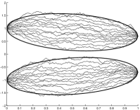
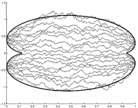
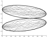
Figure 1: $n=20$ non-intersecting Brownian motions at temperature $T=1$ with two starting and two ending positions in the case of (a) large, (b) small, and (c) critical separation between the endpoints. The horizontal axis stands for the time, $t\in[0,1]$, and the vertical axis shows the positions of the Brownian motions at time $t$. For $n\to\infty$ the Brownian motions fill a prescribed region in the time-space plane which is bounded by the boldface lines in the figure. In the case (c), the limiting support consists of two touching ellipses which touch each other at a critical point which is a tacnode.

The goal of this paper is to extend the approach of [13] to a hard-edge situation. To this end we consider a model of non-intersecting squared Bessel paths [12], see also [31, 32, 27, 28, 29]. In the critical case we can get a situation where the limiting hull of the paths is touching the hard edge at a certain critical time $t^{*}$. This is shown in the third and fourth picture of Figure 2. We will refer to the touching point as a hard-edge tacnode. (This is an analogue of the higher-order tacnode in the classification scheme in [33, p. 72].) We will see that the microscopic behavior of the paths near the hard-edge tacnode is again expressed by a limiting kernel defined in terms of a $4\times 4$ RH problem, which is now related to the Hastings-McLeod solution to the inhomogeneous Painlevé II equation.

Our scaling limit near the hard-edge tacnode will be more general than the one in [13]. In the latter paper we used a $O(n^{-2/3})$ scaling of the endpoints, or equivalently of the temperature $T$. In the present paper we will use an extra $O(n^{-1/3})$ scaling of the time $t$, similarly to [2, 14, 24]. At the level of the RH problem this leads to an extra parameter $\tau$, as in [14]. While the extension of the RH problem with the parameter $\tau$ was already known to the authors of [13], the solvability of the extended RH problem is a quite non-trivial fact. This solvability was recently established by Duits and Geudens in the symmetric case [14]. We will make use of their ideas. We note that the solvability of the extended RH problem in the general non-symmetric case has not been settled yet.

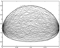
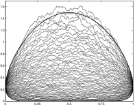
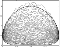
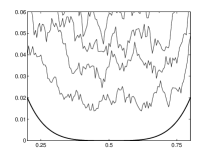
Figure 2: $n=50$ non-intersecting squared Bessel paths at temperature $T=1$ starting in $a>0$ and ending in $b>0$ with (a) $a=b=2$, (b) $a=b=0.25$, and (c) $a=b=0.5$, illustrating the case of large, small and critical ending positions, respectively. In the case (c), the paths are tangent to the hard edge at time $t^{*}=1/2$ (hard-edge tacnode) with a fourth order contact. A magnified picture near the hard-edge tacnode is shown in (d).

Now we describe our model in more detail, following [12]. Let $X(\tau)$ be a squared Bessel process with parameter $\alpha>-1$, i.e., a diffusion process (a strong Markov process on $\mathbb{R}$ with continuous sample paths) with transition probability density [26, 30]

$$p_{\tau}^{\alpha}(x,y) =\frac{1}{2\tau}\left(\frac{y}{x}\right)^{\alpha/2}e^{-\frac{x+y}{2\tau}}I_{\alpha}\left(\frac{\sqrt{xy}}{\tau}\right), \qquad x,y>0,$$ (1.1)

$$p_{\tau}^{\alpha}(0,y) =\frac{y^{\alpha}}{(2\tau)^{\alpha+1}\Gamma(\alpha+1)}e^{-\frac{y}{2\tau}}, \qquad y>0,$$ (1.2)

where $\tau$ stands for the time, $x,y$ for the position and where

$$I_{\alpha}(z)=\sum_{k=0}^{\infty}\frac{(z/2)^{2k+\alpha}}{k!\Gamma(k+\alpha+1)}$$ (1.3)

is the modified Bessel function of the first kind of order $\alpha$; see [1, p.375]. If $d=2(\alpha+1)$ is an integer, the squared Bessel process behaves like the square of the distance to the origin of a $d$-dimensional Brownian motion. Some applications of this diffusion process in mathematical finance and other fields can be found in [26], see also [19, 28, 29, 34].

We will consider $n$ independent squared Bessel processes $X_{j}(\tau)$, $j=1,\ldots,n$. It is then convenient to perform a rescaling of the time $\tau\mapsto t$ by

$$\tau=\frac{T}{2n}t.$$ (1.4)

The proportionality parameter $T>0$ can be interpreted as the temperature. It has a natural physical interpretation, in the sense that high temperature corresponds to a large variance of the squared Bessel process and vice versa.

We consider a model of $n$ independent squared Bessel processes, starting in $a>0$ at time $t=0$, ending in $b>0$ at time $t=1$, and conditioned (in the sense of Doob) not to intersect in the whole time interval $t\in(0,1)$. This model was studied by Kuijlaars, Martínez-Finkelshtein and Wielonsky [31, 32] for $b=0$ and for general $a,b>0$ in the non-critical case in [12]. We also mention the large deviation principle recently established for a closely related model in [20].

Let us fix the temperature $T=1$. There are three cases to distinguish, see Figure 2. If $ab>1/4$ then the paths do not reach the hard edge at the origin. If $ab<1/4$ then they hit the hard edge and stick to it during a certain time interval $[t_{1},t_{2}]$. Finally, for the critical separation $ab=1/4$ the paths are touching to the hard edge at one particular time $t=t^{*}\in[0,1]$, given by

$$t^{*}=\frac{\sqrt{a}}{\sqrt{a}+\sqrt{b}}.$$ (1.5)

These three cases are illustrated in Figure 2(a)–(c).

\begin{overpic}[scale={0.27}]{PhaseDiagram}\put(42.0,50.0){Case III} \put(13.5,50.0){Case II} \put(77.0,50.0){Case II} \put(46.0,26.0){Case I} \end{overpic}

Figure 3: Phase diagram in the $(t,T)$ plane for the non-intersecting squared Bessel paths with $a=b=1/2$. The critical tacnode point is located at $(t,T)=(1/2,1)$.

In this paper we find it convenient to take fixed endpoints $a,b$ satisfying $ab=1/4$. We consider the time $t\in[0,1]$ and temperature $T>0$ to be varying. Figure 3 shows the phase diagram in the $(t,T)$-plane if $a=b=1/2$. The diagram shows three regions. Case I corresponds to temperature $T<1$. Then the paths do not reach the hard edge and at each fixed time $t\in(0,1)$ they are asymptotically distributed on the interval $[p,q]=[p(t),q(t)]$ with [12, Sec. 4.3]

$$\sqrt{p}:= (1-t)\sqrt{a}+t\sqrt{b}-\sqrt{2t(1-t)T}>0,$$ (1.6)

$$\sqrt{q}:= (1-t)\sqrt{a}+t\sqrt{b}+\sqrt{2t(1-t)T}.$$ (1.7)

The limiting density of the paths on $[p,q]$ is the Marcenko-Pastur density [12, Remark 1].

In Cases II and III we have $T>1$, with the paths reaching the hard edge in Case III and staying away from it in Case II. The limiting density is a transformation of the one in [7]; it is different from the Marcenko-Pastur density. We note that the limiting density and support are always independent of $\alpha$.

The critical curves in the phase diagram are exactly like in the corresponding model of non-intersecting Brownian motions [11, Sec. 1.9], thanks to [12, Remark 1]. But the nature of the phase transitions is different due to the presence of the hard edge.

At the transition of Cases I and II we expect a phase transition in terms of the inhomogeneous Painlevé II equation (2.13) with $\nu=\alpha+1/2$. This transition may not be felt in the correlation kernel but should certainly manifest itself in the critical limits of the recurrence coefficients of the multiple orthogonal polynomials, as in [11]. At the transition of Cases II and III we expect the same phase transition as in [32]. We note that the transition curve is given by the equation [11, Sec. 1.9]

$$T=\frac{a(1-t)^{2}+bt^{2}}{t(1-t)}.$$ (1.8)

The topic of the present paper is the multi-critical tacnode point $(t,T)=(t^{*},1)$ which lies at the transition of each of the Cases I, II and III in the phase diagram.

2 Statement of results

2.1 A new $4\times 4$ Riemann-Hilbert problem

We introduce a new $4\times 4$ RH problem, which is a variant of the RH problem in [13, 14]. The RH problem generalizes the one in [13, 14] in the sense that it contains non-trivial ‘Stokes multipliers’ $e^{\nu\pi i}$ and $e^{-\nu\pi i}$. As in [14] we also have an extra parameter $\tau$.

The RH problem will have jumps on a contour in the complex plane consisting of $10$ rays emanating from the origin. More precisely, let us fix two numbers $\varphi_{1},\varphi_{2}$ such that

$$0<\varphi_{1}<\varphi_{2}<\pi/2.$$ (2.1)

Then we define the half-lines $\Gamma_{k}$, $k=0,\ldots,9$, by

$$\Gamma_{0}=\mathbb{R}_{+},\quad\Gamma_{1}=e^{i\varphi_{1}}\mathbb{R}_{+},\quad\Gamma_{2}=e^{i\varphi_{2}}\mathbb{R}_{+},\quad\Gamma_{3}=e^{i(\pi-\varphi_{2})}\mathbb{R}_{+},\quad\Gamma_{4}=e^{i(\pi-\varphi_{1})}\mathbb{R}_{+},$$ (2.2)

and

$$\Gamma_{5+k}=-\Gamma_{k},\qquad k=0,\ldots,4.$$ (2.3)

All rays $\Gamma_{k}$, $k=0,\ldots,9$, are oriented towards infinity, as shown in Figure 4. We also denote by $\Omega_{k}$ the region in $\mathbb{C}$ which lies between the rays $\Gamma_{k}$ and $\Gamma_{k+1}$, for $k=0,\ldots,9$, where we identify $\Gamma_{10}:=\Gamma_{0}$.

Using this definition of the rays $\Gamma_{k}$, we now consider the following RH problem.

Figure 4: The figure shows the jump contours $\Gamma_{k}$ in the complex $\zeta$-plane and the corresponding jump matrix $J_{k}$ on $\Gamma_{k}$, $k=0,\ldots,9$, in the RH problem for $M=M(\zeta)$. We denote by $\Omega_{k}$ the region between the rays $\Gamma_{k}$ and $\Gamma_{k+1}$.

RH problem 2.1.

We look for a $4\times 4$ matrix valued function $M(\zeta)$ (which also depends parametrically on $\nu>-1/2$ and on the complex parameters $r_{1},r_{2},s,\tau\in\mathbb{C}$) satisfying

• $M(\zeta)$ is analytic for $\zeta\in\mathbb{C}\setminus\left(\bigcup_{k=0}^{9}\Gamma_{k}\right)$.

• For $\zeta\in\Gamma_{k}$, the limiting values

  $$M_{+}(\zeta)=\lim_{z\to\zeta,\,z\textrm{ on $+$-side of }\Gamma_{k}}M(z),\qquad M_{-}(\zeta)=\lim_{z\to\zeta,\,z\textrm{ on $-$-side of }\Gamma_{k}}M(z)$$

  exist, where the $+$-side and $-$-side of $\Gamma_{k}$ are the sides which lie on the left and right of $\Gamma_{k}$, respectively, when traversing $\Gamma_{k}$ according to its orientation. These limiting values satisfy the jump relation

  $$M_{+}(\zeta)=M_{-}(\zeta)J_{k}(\zeta),\qquad k=0,\ldots,9,$$ (2.4)

  where the jump matrix $J_{k}(\zeta)$ for each ray $\Gamma_{k}$ is shown in Figure 4.

• As $\zeta\to\infty$ we have

  $$M(\zeta)=\left(I+\frac{M_{1}}{\zeta}+\frac{M_{2}}{\zeta^{2}}+O\left(\frac{1}{\zeta^{3}}\right)\right)\operatorname{diag}((-\zeta)^{-1/4},\zeta^{-1/4},(-\zeta)^{1/4},\zeta^{1/4})\\ \times\mathcal{A}\operatorname{diag}\left(e^{-\theta_{1}(\zeta)+\tau\zeta},e^{-\theta_{2}(\zeta)-\tau\zeta},e^{\theta_{1}(\zeta)+\tau\zeta},e^{\theta_{2}(\zeta)-\tau\zeta}\right),$$ (2.5)

  where the coefficient matrices $M_{1},M_{2},\ldots$ are independent of $\zeta$, and with

  $$\mathcal{A}:=\frac{1}{\sqrt{2}}\begin{pmatrix}1&0&-i&0\\ 0&1&0&i\\ -i&0&1&0\\ 0&i&0&1\\ \end{pmatrix},$$ (2.6)

  $$\theta_{1}(\zeta)=\frac{2}{3}r_{1}(-\zeta)^{3/2}+2s(-\zeta)^{1/2},\qquad\theta_{2}(\zeta)=\frac{2}{3}r_{2}\zeta^{3/2}+2s\zeta^{1/2}.$$ (2.7)

  Here we use the principal branches of the fractional powers, i.e., $\zeta^{a}:=|\zeta|^{a}e^{ia\arg\zeta}$ with argument function $|\arg\zeta|<\pi$, for any $a\in\mathbb{R}$. Note that $\zeta^{a}$ and $(-\zeta)^{a}$ have a branch cut for $\zeta$ along the negative and positive real line respectively.

• As $\zeta\to 0$ we have

  $$M(\zeta)=O(\zeta^{\nu}),\quad M^{-1}(\zeta)=O(\zeta^{\nu}), \qquad\hbox{if $\nu\leq 0$},$$ (2.8)

  and

  $$\left\{\begin{array}[]{ll}M(\zeta)\operatorname{diag}(\zeta^{-\nu},\zeta^{\nu},\zeta^{\nu},\zeta^{-\nu})=O(1),&\quad\zeta\in\Omega_{1}\cup\Omega_{8},\\ M(\zeta)\operatorname{diag}(\zeta^{\nu},\zeta^{-\nu},\zeta^{-\nu},\zeta^{\nu})=O(1),&\quad\zeta\in\Omega_{3}\cup\Omega_{6},\\ M(\zeta)=O(\zeta^{-\nu}),&\quad\textrm{elsewhere,}\end{array}\right.\hbox{if $\nu\geq 0$},$$ (2.12)

  where the $O$-symbol is defined entrywise.

More detailed information on the behavior of $M(\zeta)$ for $\zeta\to 0$ is given in Proposition 5.3.

It follows from standard arguments (e.g. [8]) that the solution to the RH problem 2.1 is unique if it exists. The existence of the solution is non-trivial and is stated in the following theorem, whose proof will be given in Section 6.

Theorem 2.2.

(Existence). Assume $\nu>-1/2$, $r_{1}=r_{2}=:r>0$, $s,\tau\in\mathbb{R}$. Then the RH problem 2.1 for $M(\zeta)$ is uniquely solvable. The same is true when $r_{1},r_{2},s,\tau$ belong to a sufficiently small complex neighborhood of the above values.

The next theorem provides a connection with the inhomogeneous Painlevé II equation

$$q^{\prime\prime}(x)=xq(x)+2q^{3}(x)-\nu,$$ (2.13)

where the prime denotes the derivative with respect to $x$. The Hastings-McLeod solution [17, 21] is the special solution $q(x)$ of (2.13) which is real for real $x$ and satisfies

$$q(x)\sim\frac{\nu}{x}\qquad x\to+\infty,$$ (2.14)

$$q(x)\sim\sqrt{\frac{-x}{2}}\qquad x\to-\infty.$$ (2.15)

We also define the Hamiltonian $u(x)$ by

$$u(x):=(q^{\prime}(x))^{2}-xq^{2}(x)-q^{4}(x)+2\nu q(x)$$ (2.16)

and note that

$$u^{\prime}(x)=-q^{2}(x).$$ (2.17)

Theorem 2.3.

($M_{1}$ vs. the Painlevé II equation). Let the parameters $\nu>-1/2$, $r_{1}=r_{2}=1$, $s,\tau\in\mathbb{R}$ in (2.5)–(2.7) be fixed. The residue matrix $M_{1}$ in (2.5) takes the form

$$M_{1}=\begin{pmatrix}a&b&ic&id\\ -b&-a&id&ic\\ ie&if&-g&h\\ if&ie&-h&g\end{pmatrix}$$ (2.18)

where $a,b,c,\ldots$ are real valued constants depending on $\nu$, $s$ and $\tau$. We have

$$d =2^{-1/3}q\left(2^{2/3}(2s-\tau^{2})\right),$$ (2.19)

$$c =-2^{-1/3}u(2^{2/3}(2s-\tau^{2}))+s^{2},$$ (2.20)

with $q$ the Hastings-McLeod solution to the inhomogeneous Painlevé II equation (2.13)–(2.15), and with $u$ the Hamiltonian in (2.16).

Theorem 2.3 will be proved in Section 5. In the homogeneous case $\nu=0$ the theorem recovers some results from [13], see also [14]. In the proof we also obtain identities relating the other entries of $M_{1}$ in terms of the entries $c$ and $d$, see e.g. (6.2). We trust that the notations $a,b$ in (2.18) will not lead to confusion with the endpoints of the squared Bessel paths.

The most difficult part of Theorem 2.3 is proving that $q(x)$ is precisely the Hastings-McLeod solution to the Painlevé II equation. This will require asymptotic results that we derive in Sections 3 and 4.

Finally, we transform the RH matrix $M(\zeta)$ into a new matrix $\widehat{M}(\zeta)$ as follows

$$\widehat{M}(\zeta):=\operatorname{diag}(\zeta^{1/4},\zeta^{-1/4},\zeta^{1/4},\zeta^{-1/4})\operatorname{diag}\left(\begin{pmatrix}1&-1\\ 1&1\end{pmatrix},\begin{pmatrix}1&1\\ -1&1\end{pmatrix}\right)M(\zeta^{1/2}).$$ (2.21)

The transformed matrix $\widehat{M}(\zeta)$ depends on the same parameters $r_{1},r_{2},s,\tau,\nu$ as $M(\zeta)$. The matrix $\widehat{M}(\zeta)$ satisfies a RH problem by itself but we will not state it here.

2.2 Critical asymptotics of squared Bessel paths

Now we describe the critical asymptotics of the non-intersecting squared Bessel paths. We will work under the triple scaling limit where the endpoints $a$, $b$ are fixed such that

$$ab=1/4.$$ (2.22)

We will let the time $t$ and the temperature $T$ depend on $n$ such that

$$t = \frac{\sqrt{a}}{\sqrt{a}+\sqrt{b}}+Kn^{-1/3},$$ (2.23)

$$T = 1+Ln^{-2/3},$$ (2.24)

where $K,L$ are arbitrary real constants.

Denote again by $\alpha$ the parameter of the non-intersecting squared Bessel paths. It turns out that under the scaling limit (2.22)–(2.24), the analysis of the squared Bessel paths for large $n$ leads to the RH problem 2.1, with the parameters $r_{1}=r_{2}=1$ and with $\nu$, $s=s^{*}$ and $\tau=\tau^{*}$ given by

$$\nu =\alpha+1/2,$$ (2.25)

$$s^{*} =\frac{K^{2}(\sqrt{a}+\sqrt{b})^{4}-L}{2},$$ (2.26)

$$\tau^{*} =-K(\sqrt{a}+\sqrt{b})^{2}.$$ (2.27)

For $u,v>0$, we define the tacnode kernel $K^{tacnode}(u,v;s^{*},\tau^{*},\alpha)$ as

$$K^{tacnode}(u,v;s^{*},\tau^{*},\alpha)=\frac{1}{2\pi i(u-v)}\begin{pmatrix}-1&0&1&0\end{pmatrix}\widehat{M}_{+}^{-1}(v)\widehat{M}_{+}(u)\begin{pmatrix}1&0&1&0\end{pmatrix}^{T},$$ (2.28)

where the superscript ^T stands for the transpose. Here $\widehat{M}(\zeta)$ is defined in (2.21) where the RH matrix $M(\zeta)$ is defined with respect to the parameters $r_{1}=r_{2}=1$, $s=s^{*}$, $\tau=\tau^{*}$ and $\nu:=\alpha+1/2.$

The squared Bessel paths at each fixed time $t\in(0,1)$ are a determinantal point process with correlation kernel $K_{n}(x,y)$, see Section 2.3 below. Now we state our main result.

Theorem 2.4.

(Asymptotics of the correlation kernel). Consider $n$ non-intersecting squared Bessel paths on the time interval $[0,1]$ with transition probability density (1.1)–(1.4) with given starting point $a>0$ and given endpoint $b>0$. Assume that (2.22)–(2.24) hold. Then the correlation kernel $K_{n}$ for the positions of the paths at time $t$ has the following scaling limit as $n\to\infty$ with $n$ even,

$$\lim_{n\to\infty}\frac{1}{\kappa^{2}n^{4/3}}K_{n}\left(\frac{u}{\kappa^{2}n^{4/3}},\frac{v}{\kappa^{2}n^{4/3}}\right)=u^{\alpha/2}v^{-\alpha/2}K^{tacnode}(u,v;s^{*},\tau^{*},\alpha),$$ (2.29)

for any fixed $u,v>0$, where $s^{*}$ and $\tau^{*}$ are given in (2.26)–(2.27) and with

$$\kappa=2(\sqrt{a}+\sqrt{b}).$$ (2.30)

We expect the conclusion of Theorem 2.4 to remain valid if $n\to\infty$ with $n$ odd.

Note that the factor $u^{\alpha/2}v^{-\alpha/2}$ in (2.29) has no influence on the correlation functions of the determinantal point process induced by $K^{tacnode}$. Moreover, when comparing $K^{tacnode}$ to the kernel in [13, Eq. (2.48)], note that the latter has a typo: it has ‘$M_{+}^{-1}(u)M_{+}(v)$’ instead of ‘$M_{+}^{-1}(v)M_{+}(u)$’.

Remark 2.5.

(Varying endpoints). Fix $a^{*},b^{*}>0$ such that $a^{*}b^{*}=1/4$ and assume that the endpoints $a,b$ vary with $n$ as

$$a =a^{*}(1+2L_{1}n^{-2/3}),$$ (2.31)

$$b =b^{*}(1+2L_{2}n^{-2/3}),$$ (2.32)

for certain real constants $L_{1},L_{2}$. Assume again that the time $t$ and temperature $T$ vary with $n$ as in (2.23)–(2.24), but with $a,b$ replaced by $a^{*},b^{*}$. Then the conclusion of Theorem 2.4 remains valid, with now (2.26) replaced by

$$s^{*} =\frac{K^{2}(\sqrt{a}+\sqrt{b})^{4}-L+L_{1}+L_{2}}{2}.$$ (2.33)

Remark 2.6.

(Bessel process). Theorem 2.4 was formulated for the squared Bessel process (1.1)–(1.4). By taking square roots, one obtains a similar statement for the (ordinary) Bessel process. The correlation kernel $\widetilde{K}_{n}(x,y)$ for the positions of $n$ non-intersecting Bessel processes on $[0,1]$, starting at $\sqrt{a}$ and ending at $\sqrt{b}$, is expressed in terms of the above $K_{n}$ by

$$\widetilde{K}_{n}(x,y)=2\sqrt{xy}K_{n}(x^{2},y^{2}),$$

see [31, Remark 2.10]. The analogue of (2.29) in this case is

$$\lim_{n\to\infty}\frac{1}{\kappa n^{2/3}}\widetilde{K}_{n}\left(\frac{u}{\kappa n^{2/3}},\frac{v}{\kappa n^{2/3}}\right)=2u^{\alpha}v^{-\alpha}\sqrt{uv}K^{tacnode}(u^{2},v^{2};s^{*},\tau^{*},\alpha).$$ (2.34)

Remark 2.7.

(Chiral 2-matrix model). The RH problem 2.1 for $M(\zeta)$ was recently used to study a critical phenomenon in the chiral 2-matrix model [10]. This leads to a critical correlation kernel which is essentially different from the kernel $K^{tacnode}$ in (2.28) and which is a hard edge analogue of the Duits-Geudens kernel [14].

2.3 About the proof

The positions of the non-intersecting squared Bessel paths at each particular time $t\in(0,1)$ constitute a determinantal point process. It is a multiple orthogonal polynomial (MOP) ensemble with respect to the weight functions [12]

$$\begin{array}[]{ll}w_{1,1}(x)=x^{\frac{\alpha}{2}}e^{-\frac{nx}{Tt}}I_{\alpha}\left(\frac{2n\sqrt{ax}}{Tt}\right),&w_{1,2}(x)=x^{\frac{\alpha+1}{2}}e^{-\frac{nx}{Tt}}I_{\alpha+1}\left(\frac{2n\sqrt{ax}}{Tt}\right),\\ w_{2,1}(x)=x^{-\frac{\alpha}{2}}e^{-\frac{nx}{T(1-t)}}I_{\alpha}\left(\frac{2n\sqrt{bx}}{T(1-t)}\right),&w_{2,2}(x)=x^{-\frac{\alpha-1}{2}}e^{-\frac{nx}{T(1-t)}}I_{\alpha-1}\left(\frac{2n\sqrt{bx}}{T(1-t)}\right).\end{array}$$ (2.37)

Here $T>0$ is the temperature.

This MOP ensemble is related to the following RH problem [12].

RH problem 2.8.

We look for a $4\times 4$ matrix valued function $Y$ satisfying

1. $Y$ is analytic in $\mathbb{C}\setminus\mathbb{R}_{+}$.

2. For $x>0$, $Y$ possesses continuous boundary values $Y_{+}$ (from the upper half plane) and $Y_{-}$ (from the lower half plane), which satisfy

   $$Y_{+}(x)=Y_{-}(x)\begin{pmatrix}I_{2}&W(x)\\ 0&I_{2}\end{pmatrix},$$ (2.38)

   where $I_{k}$ denotes the identity matrix of size $k$ and $W(x)$ is the rank-one matrix

   $$W(x)=\begin{pmatrix}w_{1,1}(x)&w_{1,2}(x)\end{pmatrix}^{T}\begin{pmatrix}w_{2,1}(x)&w_{2,2}(x)\end{pmatrix}.$$

3. As $z\to\infty$, $z\in\mathbb{C}\setminus\mathbb{R}_{+}$, we have

   $$Y(z)=(I+O(1/z))~{}\operatorname{diag}(z^{n_{1}},z^{n_{2}},z^{-n_{1}},z^{-n_{2}}),$$

   where $n_{1}:=\lceil n/2\rceil$ and $n_{2}:=n-n_{1}$.

4. $Y(z)$ has the following behavior near the origin:

   $$Y(z)\operatorname{diag}(1,1,h^{-1}(z),h^{-1}(z))=O(1),\quad Y^{-T}(z)\operatorname{diag}(h^{-1}(z),1,1,1)=O(1),$$

   as $z\to 0$, $z\in\mathbb{C}\setminus\mathbb{R}_{+}$, where the $O$-symbol is defined entrywise, where the superscript ^-T denotes the inverse transpose and with

   $$h(z)=\left\{\begin{array}[]{ll}|z|^{\alpha},&\quad\hbox{if $-1<\alpha<0$,}\\ \log|z|,&\quad\hbox{if $\alpha=0$,}\\ 1,&\quad\hbox{if $\alpha>0$}.\end{array}\right.$$ (2.39)

There is a unique solution $Y$ to the above RH problem. The matrix $Y$ is constructed using multiple orthogonal polynomials of mixed type with respect to the modified Bessel weights (2.37); see [6, 12]. Due to the singularity of the weight matrix near the origin, we need the condition $(4)$ to ensure the uniqueness of the solution.

The correlation kernel admits the following representation in terms of $Y$ [6, 12]:

$$K_{n}(x,y)=\frac{1}{2\pi i(x-y)}\begin{pmatrix}0&0&w_{2,1}(y)&w_{2,2}(y)\end{pmatrix}Y_{+}^{-1}(y)Y_{+}(x)\begin{pmatrix}w_{1,1}(x)&w_{1,2}(x)&0&0\end{pmatrix}^{T}.$$ (2.40)

Outline of the paper

The remainder of this paper is organized as follows. In Sections 3 and 4 we calculate the large $s$ asymptotics of the model RH problem for $M$. Section 5 proves Theorem 2.3 on the relation of $M(\zeta)$ with the inhomogeneous Painlevé II equation. Section 6 proves Theorem 2.2 on the solvability of the model RH problem. In the final Section 7 we analyze the non-intersecting squared Bessel paths near the hard-edge tacnode and we prove Theorem 2.4.

3 Asymptotics of $M(\zeta)$ for $s\to+\infty$

In this and the next section we will analyze the model RH problem 2.1 for $M(\zeta)$ if $r_{1}=r_{2}=1$ and $\tau=0$ in the limit $s\to\infty$. We will prove the solvability of the RH problem for $s\in\mathbb{R}$ with $|s|$ sufficiently large, and also establish the large $s$ asymptotics for the quantities $c$ and $d$ in (2.18). More precisely, we will prove the following proposition.

Proposition 3.1.

Let $\nu>-1/2$ be fixed and suppose that $r_{1}=r_{2}=1$ and $\tau=0$. Then for $s\in\mathbb{R}$ with $|s|$ large enough, the RH problem for $M(\cdot)$ is uniquely solvable.

Moreover, the numbers $d=-i\left(M_{1}\right)_{1,4}$ and $c=-i\left(M_{1}\right)_{1,3}$ in (2.18) have the large $s$ asymptotics

$$d = \frac{\nu}{4s}+O(s^{-5/2}),\qquad s\to+\infty,$$ (3.1)

$$c = s^{2}+O(s^{-1}),\qquad s\to+\infty,$$ (3.2)

$$d = \sqrt{-s}+O(s^{-1}),\qquad s\to-\infty.$$ (3.3)

Proposition 3.1 will be needed in the proofs of Theorems 2.2 and 2.3. Note that in [13] we had a stronger variant of (3.1) with $\nu=0$. This stronger variant allowed us to conclude directly that $q$ in (2.19) is the Hastings-McLeod solution to Painlevé II. In contrast, the condition (3.1) is insufficient to characterize the Hastings-McLeod solution, for any parameter $\nu>-1/2$, which is why we also need the asymptotics (3.3) for $s\to-\infty$. Actually, it is possible to characterize the Hastings-McLeod solution from its behavior for $s\to+\infty$ alone (without the need for $s\to-\infty$ asymptotics) [17, Sec. 11.7]; but the latter requires an extremely detailed asymptotic analysis that is hard to perform in our setting.

The proof of Proposition 3.1 is based on the Deift-Zhou steepest descent analysis of the RH problem for $M(\zeta)$. In this section we will perform the analysis for $s\to+\infty$, in the next section we will consider the case where $s\to-\infty$.

We now turn to the analysis for $s\to+\infty$. We will apply a series of transformations $M\mapsto A\mapsto B\mapsto C\mapsto D$, so that the matrix-valued function $D$ tends uniformly to the identity matrix as $s\to+\infty$. The transformations will be very similar to [13, Sec. 3] and therefore we only give a brief description. The main difference with [13] is in the construction of a local parametrix at the origin with the help of modified Bessel functions; see Section 3.4.

3.1 First transformation: $M\mapsto A$

The first three transformations will be almost identical as in [13, Sec. 3]. The first transformation $M\mapsto A$ is a rescaling of the RH problem for $M$:

$$A(\zeta)=\operatorname{diag}(s^{1/4},s^{1/4},s^{-1/4},s^{-1/4})M(s\zeta),\qquad\zeta\in\mathbb{C}\setminus\bigcup_{k=0}^{9}\Gamma_{k}.$$ (3.4)

The matrix $A$ satisfies a RH problem with exactly the same jumps and behavior near the origin as $M(\zeta)$. The large $\zeta$ asymptotics in (2.5) changes to

$$A(\zeta)=\left(I+\frac{A_{1}}{\zeta}+O\left(\frac{1}{\zeta^{2}}\right)\right)\operatorname{diag}((-\zeta)^{-1/4},\zeta^{-1/4},(-\zeta)^{1/4},\zeta^{1/4})\\ \times\mathcal{A}\operatorname{diag}\left(e^{-\lambda\tilde{\theta}_{1}(\zeta)},e^{-\lambda\tilde{\theta}_{2}(\zeta)},e^{\lambda\tilde{\theta}_{1}(\zeta)},e^{\lambda\tilde{\theta}_{2}(\zeta)}\right)$$ (3.5)

with $\mathcal{A}$ as in (2.6) and with

$$\lambda=s^{3/2},\qquad\tilde{\theta}_{1}(\zeta)=\frac{2}{3}(-\zeta)^{3/2}+2(-\zeta)^{1/2},\qquad\quad\tilde{\theta}_{2}(\zeta)=\frac{2}{3}\zeta^{3/2}+2\zeta^{1/2}.$$ (3.6)

3.2 Second transformation: $A\mapsto B$

Figure 5: Jump contour $\Sigma_{B}$ for the RH problem for $B$. Note the reversion of the orientation of the rays $\tilde{\Gamma}_{4}$, $\tilde{\Gamma}_{6}$ and $(-\infty,0)$.

In the second transformation we apply contour deformations. The four rays $\Gamma_{k}$, $k=1,4,6,9$, emanating from the origin are replaced by their parallel lines emanating from some special points on the real line. More precisely, we replace $\Gamma_{1}$ and $\Gamma_{9}$ by their parallel rays $\tilde{\Gamma}_{1}$ and $\tilde{\Gamma}_{9}$ emanating from the point $2$, and replace $\Gamma_{4}$ and $\Gamma_{6}$ by their parallel rays $\tilde{\Gamma}_{4}$ and $\tilde{\Gamma}_{6}$ emanating from the point $-2$. See Figure 5.

Denote by $E_{j,k}$ the $4\times 4$ elementary matrix with entry $1$ at the $(j,k)$th position and all other entries equal to zero. We define

$$B(\zeta)=\left\{\begin{array}[]{ll}A(\zeta)(I+E_{3,1}),&\text{for $\zeta$ between $\Gamma_{1}$, $[0,2]$ and $\tilde{\Gamma}_{1}$},\\ A(\zeta)(I-E_{3,1}),&\text{for $\zeta$ between $\Gamma_{9}$, $[0,2]$ and $\tilde{\Gamma}_{9}$},\\ A(\zeta)(I+E_{4,2}),&\text{for $\zeta$ between $\Gamma_{4}$, $[-2,0]$ and $\tilde{\Gamma}_{4}$},\\ A(\zeta)(I-E_{4,2}),&\text{for $\zeta$ between $\Gamma_{6}$, $[-2,0]$ and $\tilde{\Gamma}_{6}$},\\ A(\zeta),&\text{elsewhere}.\end{array}.\right.$$ (3.7)

The large $\zeta$ asymptotics of $B(\zeta)$ are the same as for $A(\zeta)$, see (3.5). The new jumps of $B$ on the interval $(-2,2)$ are given by

$$B_{+}(\zeta)=B_{-}(\zeta)(I+E_{1,3}), \qquad\zeta\in(0,2),$$

$$B_{+}(\zeta)=B_{-}(\zeta)(I+E_{2,4}), \qquad\zeta\in(-2,0).$$

The jumps of $B$ on the remaining contours are the same as those for $A$, provided that $\Gamma_{j}$ is replaced by $\tilde{\Gamma}_{j}$, $j\in\{1,4,6,9\}$, and that the change of the orientation of $\tilde{\Gamma}_{4}$, $\tilde{\Gamma}_{6}$ and $(-\infty,0)$ is taken into account. (The reversion of a contour implies that the jump matrix is replaced by its inverse). The jump contour $\Sigma_{B}$ for $B(\zeta)$ is shown in Figure 5.

3.3 Third transformation: $B\mapsto C$

The third transformation is a normalization of the RH problem at infinity. Define the ‘$g$-functions’

$$g_{1}(\zeta)=\frac{2}{3}(2-\zeta)^{3/2},\qquad \zeta\in\mathbb{C}\setminus[2,\infty),$$ (3.8)

$$g_{2}(\zeta)=\frac{2}{3}(2+\zeta)^{3/2},\qquad \zeta\in\mathbb{C}\setminus(-\infty,-2],$$ (3.9)

with the principal branch of the power $3/2$. We define the transformation $B\mapsto C$ as

$$C(\zeta)=(I+i\lambda(E_{3,1}-E_{4,2}))B(\zeta)\operatorname{diag}(e^{\lambda g_{1}(\zeta)},e^{\lambda g_{2}(\zeta)},e^{-\lambda g_{1}(\zeta)},e^{-\lambda g_{2}(\zeta)}),$$ (3.10)

where again $\lambda:=s^{3/2}$. As in [13, Sec. 3.4], one shows that $C$ satisfies the following RH problem.

RH problem 3.2.

We look for a $4\times 4$ matrix valued function $C$ such that

1. $C(\zeta)$ is analytic for $\zeta\in\mathbb{C}\setminus\Sigma_{B}$.

2. $C$ has the following jumps on $\Sigma_{B}$:

   $$C_{+}(\zeta)=C_{-}(\zeta)J_{C}(\zeta),$$

   where $J_{C}$ is given by

   $$J_{C}(\zeta) =E_{2,2}+E_{4,4}+E_{1,3}-E_{3,1},\qquad\text{for $\zeta\in(2,\infty)$},$$

   $$J_{C}(\zeta) =(I+e^{2\lambda g_{1}(\zeta)}E_{3,1}),\qquad\text{for $\zeta\in\tilde{\Gamma}_{1}\cup\tilde{\Gamma}_{9}$},$$

   $$J_{C}(\zeta) =(I+e^{-2\lambda g_{1}(\zeta)}E_{1,3}),\qquad\text{for $\zeta\in(0,2)$},$$

   $$J_{C}(\zeta) =(I+e^{\lambda(g_{1}-g_{2})(\zeta)}e^{\nu\pi i}(E_{3,4}-E_{2,1})),\qquad\text{for $\zeta\in\Gamma_{2}$},$$ (3.11)

   $$J_{C}(\zeta) =(I-e^{\lambda(g_{1}-g_{2})(\zeta)}e^{-\nu\pi i}(E_{3,4}-E_{2,1})),\qquad\text{for $\zeta\in\Gamma_{8}$},$$ (3.12)

   $$J_{C}(\zeta) =(I-e^{-\lambda(g_{1}-g_{2})(\zeta)}e^{-\nu\pi i}(E_{4,3}-E_{1,2})),\qquad\text{for $\zeta\in\Gamma_{3}$},$$ (3.13)

   $$J_{C}(\zeta) =(I+e^{-\lambda(g_{1}-g_{2})(\zeta)}e^{\nu\pi i}(E_{4,3}-E_{1,2})),\qquad\text{for $\zeta\in\Gamma_{7}$},$$ (3.14)

   $$J_{C}(\zeta) =(I+e^{-2\lambda g_{2}(\zeta)}E_{2,4}),\qquad\text{for $\zeta\in(-2,0)$},$$

   $$J_{C}(\zeta) =(I+e^{2\lambda g_{2}(\zeta)}E_{4,2}),\qquad\text{for $\zeta\in\tilde{\Gamma}_{4}\cup\tilde{\Gamma}_{6}$},$$

   $$J_{C}(\zeta) =E_{1,1}+E_{3,3}+E_{2,4}-E_{4,2},\qquad\text{for $\zeta\in(-\infty,-2)$}.$$

3. As $\zeta\to\infty$, we have

   $$C(\zeta)= \left(I+\frac{C_{1}}{\zeta}+O\left(\frac{1}{\zeta^{2}}\right)\right)\operatorname{diag}((-\zeta)^{-1/4},\zeta^{-1/4},(-\zeta)^{1/4},\zeta^{1/4})\mathcal{A},$$ (3.15)

   where

   $$C_{1}=(I+i\lambda(E_{3,1}-E_{4,2}))\left[A_{1}(I-i\lambda(E_{3,1}-E_{4,2}))+\begin{pmatrix}-\frac{\lambda^{2}}{2}&0&-i\lambda&0\\ 0&\frac{\lambda^{2}}{2}&0&-i\lambda\\ \frac{i\lambda^{3}-2i\lambda}{6}&0&-\frac{\lambda^{2}}{2}&0\\ 0&\frac{i\lambda^{3}-2i\lambda}{6}&0&\frac{\lambda^{2}}{2}\end{pmatrix}\right],$$ (3.16)

   with $A_{1}$ the residue matrix in (3.5).

4. The behavior of $C(\zeta)$ for $\zeta\to 0$ is the same as for $M(\zeta)$. More precisely,

   $$\begin{array}[]{ll}C(\zeta)=O(\zeta^{\nu}),\quad C^{-1}(\zeta)=O(\zeta^{\nu}),\qquad\zeta\to 0,&\qquad\textrm{if $\nu\leq 0$},\\ C(\zeta)\operatorname{diag}(\zeta^{-\nu},\zeta^{\nu},\zeta^{\nu},\zeta^{-\nu})=O(1),\qquad\zeta\to 0,&\qquad\textrm{if $\nu\geq 0$},\end{array}$$ (3.17)

   where in the second line we assume that $\zeta\to 0$ to the right of $\Gamma_{2}$ and $\Gamma_{8}$.

As in [13] we obtain the following expressions for the numbers $c$ and $d$ in (2.18):

$$c=-i\sqrt{s}(C_{1})_{1,3}+s^{2},\qquad d=-i\sqrt{s}(C_{1})_{1,4}.$$ (3.18)

3.4 Global and local parametrices

Global parametrix

Away from the points $2$, $-2$ and $0$, we will approximate $C$ by the ‘global parametrix’

$$C^{(\infty)}(\zeta)=\operatorname{diag}\left((2-\zeta)^{-1/4},(2+\zeta)^{-1/4},(2-\zeta)^{1/4},(2+\zeta)^{1/4}\right)\mathcal{A},$$ (3.19)

with $\mathcal{A}$ as in (2.6), and where, as usual, we take the principal branches of $(2+\zeta)^{1/4}$ and $(2-\zeta)^{1/4}$ with cuts along $(-\infty,-2]$ and $[2,\infty)$, respectively. See [13, Sec. 3.6].

Local parametrices at the points $-2$ and $2$

In small neighborhoods of the points $-2$ and $2$ we construct local parametrices $C^{(-2)}$, $C^{(2)}$ to the RH problem, respectively. These parametrices are constructed with the help of Airy functions, exactly as in [13, Sec. 3.7].

Local parametrix at the origin

The next step, which has no analogue in [13, Sec. 3], is the construction of a local parametrix $C^{(0)}$ near the origin. The construction will rely on the one in [12, Sec. 5.6]. The local parametrix $C^{(0)}$ will be defined in the disk $B_{\rho}$ of radius $\rho$ around the origin in $\mathbb{C}$, with $\rho>0$ fixed and sufficiently small. It will solve the following RH problem.

RH problem 3.3.

We look for a $4\times 4$ matrix valued function $C^{(0)}$ such that

• $C^{(0)}(\zeta)$ is analytic for $\zeta\in B_{\rho}\setminus\Sigma_{B}$.

• For $\zeta\in B_{\rho}\cap(\Gamma_{2}\cup\Gamma_{3}\cup\Gamma_{7}\cup\Gamma_{8})$, we have $C^{(0)}_{+}(\zeta)=C^{(0)}_{-}(\zeta)J_{C}(\zeta)$ with $J_{C}$ given in (3.11)–(3.14). For $\zeta\in(0,\rho)$ we have

  $$C^{(0)}_{+}(\zeta)=C^{(0)}_{-}(\zeta)\times\left\{\begin{array}[]{ll}I+e^{-2\lambda g_{1}(\zeta)}E_{1,3},&\textrm{if $\nu-1/2\not\in\mathbb{Z}_{\geq 0}$},\\ I,&\textrm{if $\nu-1/2\in\mathbb{Z}_{\geq 0}$},\end{array}\right.$$ (3.20)

  and for $\zeta\in(-\rho,0)$ we have

  $$C^{(0)}_{+}(\zeta)=C^{(0)}_{-}(\zeta)\times\left\{\begin{array}[]{ll}I+e^{-2\lambda g_{2}(\zeta)}E_{2,4},&\textrm{if $\nu-1/2\not\in\mathbb{Z}_{\geq 0}$},\\ I,&\textrm{if $\nu-1/2\in\mathbb{Z}_{\geq 0}$}.\end{array}\right.$$ (3.21)

• Uniformly on the circle $|\zeta|=\rho$ we have for $\lambda\to+\infty$ that

  $$C^{(0)}(\zeta)=C^{(\infty)}(\zeta)(I+O(\lambda^{-1})).$$ (3.22)

• The behavior of $C^{(0)}(\zeta)$ for $\zeta\to 0$ is the same as for $C(\zeta)$, see (3.17).

• $C^{(0)}$ satisfies the symmetry relation

  $$C^{(0)}(-\zeta)=\begin{pmatrix}J&0\\ 0&-J\end{pmatrix}C^{(0)}(\zeta)\begin{pmatrix}J&0\\ 0&-J\end{pmatrix},\qquad\textrm{with }J:=\begin{pmatrix}0&1\\ 1&0\end{pmatrix}.$$ (3.23)

The idea behind (3.20)–(3.21) is that we can get the correct jumps $J_{C}$ as long as $\nu-1/2\not\in\mathbb{Z}_{\geq 0}$. If the latter fails then we approximate $J_{C}$ by the identity matrix for $\zeta\in(-\rho,\rho)$, but we will see that the resulting approximation error can be controlled.

Figure 6: Jump contour and enclosed sectors $\omega_{0},\ldots,\omega_{5}$ for the local parametrix $C^{(0)}$.

We will see below that the solution matrix $C^{(0)}$ indeed exists. For now, we stress the symmetry relation (3.23) and note that we have the same type of relation between the jump matrices on opposite rays. Then similarly as in Proposition 5.3 in Section 5 we can find the detailed local behavior of $C^{(0)}$ near the origin. The outcome is that if $\nu-1/2\not\in\mathbb{Z}_{\geq 0}$, then there exist an analytic matrix valued function $E$ and constant matrices $A_{k}$ such that, for the sectors $\omega_{k}$ in Figure 6, we have

$$C^{(0)}(\zeta)=E(\zeta)\operatorname{diag}(\zeta^{\nu},\zeta^{\nu},\zeta^{-\nu},\zeta^{-\nu})A_{k}\operatorname{diag}(e^{\lambda g_{1}(\zeta)},e^{\lambda g_{2}(\zeta)},e^{-\lambda g_{1}(\zeta)},e^{-\lambda g_{2}(\zeta)}),$$ (3.24)

as $\zeta\in\omega_{k}$, $k=0,\ldots,5$, with in particular

$$A_{0}=\begin{pmatrix}0&0&-1&2\cos\nu\pi\\ 2\cos\nu\pi&1&e^{-\nu\pi i}&0\\ 0&1&0&0\\ 0&0&1&0\end{pmatrix}.$$ (3.25)

Note that (3.25) is the same as the matrix $A_{1}$ in (5.7), up to an irrelevant diagonal factor $D$. In fact the calculations in both cases are virtually the same.

On the other hand, if $\nu-1/2\in\mathbb{Z}_{\geq 0}$, then there exist an analytic matrix valued function $E$ and constant matrices $A_{k}$ such that

$$C^{(0)}(\zeta)=E(\zeta)K(\zeta)A_{k}\operatorname{diag}(e^{\lambda g_{1}(\zeta)},e^{\lambda g_{2}(\zeta)},e^{-\lambda g_{1}(\zeta)},e^{-\lambda g_{2}(\zeta)}),$$ (3.26)

as $\zeta\in\omega_{k}$, $k=0,\ldots,5$, where now $K(\zeta)$ is defined in (5.9) and

$$A_{0}=E_{1,1}+E_{2,4}+E_{3,2}+E_{4,3}.$$ (3.27)

In all cases, we have for certain constants $*$ that (see Remark 5.7)

$$E(0)=\begin{pmatrix}1&0&-1&0\\ 1&0&1&0\\ 0&1&0&1\\ 0&-1&0&1\end{pmatrix}\begin{pmatrix}*&*&0&0\\ *&*&0&0\\ 0&0&*&*\\ 0&0&*&*\end{pmatrix}.$$ (3.28)

Now we turn to the construction of $C^{(0)}$. It will be convenient to consider the following ‘square root version’ $C^{(0)}_{\mathrm{sq}}$ of $C^{(0)}$:

$$C^{(0)}_{\mathrm{sq}}(\zeta)=\operatorname{diag}(\zeta^{1/4},\zeta^{-1/4},\zeta^{1/4},\zeta^{-1/4})\frac{1}{\sqrt{2}}\operatorname{diag}\left(\begin{pmatrix}1&-1\\ 1&1\end{pmatrix},\begin{pmatrix}1&1\\ -1&1\end{pmatrix}\right)C^{(0)}(\zeta^{1/2})\\ \times\operatorname{diag}(J,1,1)\operatorname{diag}(-i,1,1,-i),$$ (3.29)

where as usual we take the principal branches of all the powers, and with $J$ as in (3.23). Similarly we define $C^{(\infty)}_{\mathrm{sq}}$, by replacing $C^{(0)}$ by $C^{(\infty)}$ in (3.29), recall (3.19). We also set

$$\alpha:=\nu-1/2,\qquad\Delta^{+}:=\{z^{2}\mid z\in\Gamma_{2}\},\qquad\Delta^{-}:=\{z^{2}\mid z\in\Gamma_{8}\},$$ (3.30)

with $\Delta^{+}$ and $\Delta^{-}$ oriented towards the origin. Then $C^{(0)}_{\mathrm{sq}}$ solves the following RH problem.

RH problem 3.4.

We look for a $4\times 4$ matrix valued function $C^{(0)}_{\mathrm{sq}}$ such that

• $C^{(0)}_{\mathrm{sq}}(\zeta)$ is analytic for $\zeta\in B_{\rho^{2}}\setminus\left(\mathbb{R}\cup\Delta^{+}\cup\Delta^{-}\right)$.

• $C^{(0)}_{\mathrm{sq}}$ has the following jumps on $B_{\rho^{2}}\cap\left(\mathbb{R}\cup\Delta^{+}\cup\Delta^{-}\right)$:

  $$(C^{(0)}_{\mathrm{sq}})_{+}(\zeta)=(C^{(0)}_{\mathrm{sq}})_{-}(\zeta)J_{\mathrm{sq}}(\zeta),$$ (3.31)

  where $J_{\mathrm{sq}}$ is given by

  $$J_{\mathrm{sq}}(\zeta) =\left\{\begin{array}[]{ll}I+e^{-2\lambda g_{1}(\zeta^{1/2})}E_{2,3},&\textrm{if $\alpha\not\in\mathbb{Z}_{\geq 0}$},\\ I,&\textrm{if $\alpha\in\mathbb{Z}_{\geq 0}$},\end{array}\right.\qquad\text{for $\zeta\in(0,\rho^{2})$},$$ (3.34)

  $$J_{\mathrm{sq}}(\zeta) =(I-e^{\lambda(g_{1}-g_{2})(\zeta^{1/2})}e^{\alpha\pi i}(E_{3,4}+E_{1,2})),\qquad\text{for $\zeta\in\Delta^{+}\cap B_{\rho^{2}}$},$$

  $$J_{\mathrm{sq}}(\zeta) =(I-e^{\lambda(g_{1}-g_{2})(\zeta^{1/2})}e^{-\alpha\pi i}(E_{3,4}+E_{1,2})),\qquad\text{for $\zeta\in\Delta^{-}\cap B_{\rho^{2}}$},$$

  $$J_{\mathrm{sq}}(\zeta) =\operatorname{diag}\left(\begin{pmatrix}0&1\\ -1&0\end{pmatrix},\begin{pmatrix}0&1\\ -1&0\end{pmatrix}\right),\qquad\text{for $\zeta\in(-\rho^{2},0)$}.$$ (3.35)

• $C^{(0)}_{\mathrm{sq}}(\zeta)$ behaves near the origin $\zeta\to 0$ as follows:

  $$C^{(0)}_{\mathrm{sq}}(\zeta)=O(\zeta^{\alpha/2}),\quad(C^{(0)}_{\mathrm{sq}})^{-1}(\zeta)=O(\zeta^{\alpha/2}),\qquad\alpha<0,$$ (3.36)

  $$C^{(0)}_{\mathrm{sq}}(\zeta)=O(\log(|\zeta|)),\quad(C^{(0)}_{\mathrm{sq}})^{-1}(\zeta)=O(\log(|\zeta|)),\qquad\alpha=0,$$ (3.37)

  $$C^{(0)}_{\mathrm{sq}}(\zeta)\operatorname{diag}(\zeta^{\alpha/2},\zeta^{-\alpha/2},\zeta^{\alpha/2},\zeta^{-\alpha/2})=O(1),\qquad\alpha>0,$$ (3.38)

  where in (3.38) we assume that $\zeta\to 0$ in the region to the right of $\Delta^{+}$ and $\Delta^{-}$.

• Uniformly on the circle $|\zeta|=\rho^{2}$ we have as $\lambda\to+\infty$ that

  $$C^{(0)}_{\mathrm{sq}}(\zeta)=C_{\mathrm{sq}}^{(\infty)}(\zeta)\left(I+O\!\left(\lambda^{-1}\right)\right).$$ (3.39)

Proof.

The jumps of $C^{(0)}_{\mathrm{sq}}$ on $\Delta^{+}$, $\Delta^{-}$ and $\mathbb{R}_{+}$ easily follow from $\alpha=\nu-1/2$, (3.29) and the jumps of $C^{(0)}$. Now we check the jump on $\mathbb{R}_{-}$. With the negative real axis oriented from left to right as usual, we have

$$\left[\operatorname{diag}(\zeta^{1/4},\zeta^{-1/4},\zeta^{1/4},\zeta^{-1/4})\operatorname{diag}\left(\begin{pmatrix}1&-1\\ 1&1\end{pmatrix},\begin{pmatrix}1&1\\ -1&1\end{pmatrix}\right)C^{(0)}(\zeta^{1/2})\right]_{+}$$

$$=\left[\operatorname{diag}(\zeta^{1/4},\zeta^{-1/4},\zeta^{1/4},\zeta^{-1/4})\operatorname{diag}\left(\begin{pmatrix}1&-1\\ 1&1\end{pmatrix},\begin{pmatrix}1&1\\ -1&1\end{pmatrix}\right)\right]_{-}i\operatorname{diag}\left(-J,J\right)[C^{(0)}(\zeta^{1/2})]_{+}.$$

On account of the symmetry (3.23), we obtain

$$=\left[\operatorname{diag}(\zeta^{1/4},\zeta^{-1/4},\zeta^{1/4},\zeta^{-1/4})\operatorname{diag}\left(\begin{pmatrix}1&-1\\ 1&1\end{pmatrix},\begin{pmatrix}1&1\\ -1&1\end{pmatrix}\right)C^{(0)}(\zeta^{1/2})\right]_{-}i\operatorname{diag}\left(-J,J\right).$$

By using this in (3.29), it is then straightforward to obtain the jump (3.31)–(3.35).

The behavior of $C^{(0)}_{\mathrm{sq}}(\zeta)$ as $\zeta\to 0$ follows from $\alpha=\nu-1/2$, (3.29) and a careful inspection of (3.24)–(3.28). ∎

The properties of $C^{(0)}_{\mathrm{sq}}$ and $C^{(\infty)}_{\mathrm{sq}}$ are exactly like those for ‘$T$’ and ‘$N_{\alpha}$’ in [12, Sec. 5.6], respectively, where we are dealing with ‘Case I’. We use the construction in that paper to build the matrix $C^{(0)}_{\mathrm{sq}}$ solving the RH problem 3.4, see also [10, Sec. 5.6].

Note that for $\alpha\in\mathbb{Z}_{\geq 0}$ the RH problem for $C^{(0)}_{\mathrm{sq}}$ basically decouples into two RH problems of size $2\times 2$ which can be solved using modified Bessel functions. On the other hand, if $\alpha\not\in\mathbb{Z}_{\geq 0}$ then we have a genuine $4\times 4$ RH problem and its solution requires some nontrivial modifications [12, Sec. 5.6]. In the latter paper we use these modifications only if $\alpha<0$; but the same construction works as long as $\sin(\pi\alpha)\neq 0$, i.e., $\alpha\not\in\mathbb{Z}$.

Finally, we lift $C^{(0)}_{\mathrm{sq}}$ back to the original setting by inverting (3.29): we put

$$C^{(0)}(\zeta)=\frac{1}{\sqrt{2}}\operatorname{diag}\left(\begin{pmatrix}1&1\\ -1&1\end{pmatrix},\begin{pmatrix}1&-1\\ 1&1\end{pmatrix}\right)\operatorname{diag}(\zeta^{-1/2},\zeta^{1/2},\zeta^{-1/2},\zeta^{1/2})C^{(0)}_{\mathrm{sq}}(\zeta^{2})\\ \times\operatorname{diag}(i,1,1,i)\operatorname{diag}(J,1,1),$$ (3.40)

if $\mathrm{Re}\,\zeta>0$, and

$$C^{(0)}(\zeta)=\operatorname{diag}(J,-J)C^{(0)}(-\zeta)\operatorname{diag}(J,-J),\qquad\textrm{if }\mathrm{Re}\,\zeta<0,$$

recall (3.23). We claim that this matrix satisfies the RH problem 3.3 for $C^{(0)}$. It is easily seen that it has the right jumps. It also satisfies (3.22) and (3.23). It remains to check the behavior of $C^{(0)}$ near the origin. Recall that $C^{(0)}(\zeta)$ should have the same behavior for $\zeta\to 0$ as $C(\zeta)$ in (3.17). Let us check this if $\nu<0$. It is clear from (3.40) that $C^{(0)}(\zeta)=O(\zeta^{\nu-1})$. Then we can again derive the formulas (3.24)–(3.28), with now each term $\zeta^{\nu}$ or $\zeta^{-\nu}$ replaced by $\zeta^{\nu-1}$ or $\zeta^{-\nu-1}$ respectively. Using these formulas together with (3.29) and (3.36) we see that all the entries of $E(\zeta)$ have a zero at $\zeta=0$ and so each term $\zeta^{\nu-1}$ or $\zeta^{-\nu-1}$ can be replaced by $\zeta^{\nu}$ or $\zeta^{-\nu}$ respectively, which yields the desired conclusion. Similar arguments apply if $\nu\geq 0$.

3.5 Fourth transformation: $C\mapsto D$

We define the fourth transformation

$$D(\zeta)=\left\{\begin{array}[]{ll}C(\zeta)(C^{(-2)})^{-1}(\zeta),&\text{if $|\zeta+2|<\rho$,}\\ C(\zeta)(C^{(2)})^{-1}(\zeta),&\text{if $|\zeta-2|<\rho$,}\\ C(\zeta)(C^{(0)})^{-1}(\zeta),&\text{if $|\zeta|<\rho$,}\\ C(\zeta)(C^{(\infty)})^{-1}(\zeta),&\text{elsewhere.}\end{array}\right.$$ (3.41)

Then $D$ satisfies the following RH problem.

RH problem 3.5.

We look for a $4\times 4$ matrix valued function $D$ such that

1. $D$ is analytic in $\mathbb{C}\setminus\Sigma_{D}$, where $\Sigma_{D}$ is shown in Figure 7.

2. $D$ has jumps $D_{+}(\zeta)=D_{-}(\zeta)J_{D}(\zeta)$ for $\zeta\in\Sigma_{D}$, where

   $$J_{D}=\left\{\begin{array}[]{ll}C^{(-2)}\left(C^{(\infty)}\right)^{-1},&\text{on $|\zeta+2|=\rho$,}\\ C^{(0)}\left(C^{(\infty)}\right)^{-1},&\text{on $|\zeta|=\rho$,}\\ C^{(2)}\left(C^{(\infty)}\right)^{-1},&\text{on $|\zeta-2|=\rho$,}\\ C^{(\infty)}J_{C}\left(C^{(\infty)}\right)^{-1},&\text{on the rest of $\Sigma_{D}$}.\end{array}\right.$$ (3.42)

3. As $\zeta\to\infty$, we have

   $$D(\zeta)=I+\frac{D_{1}}{\zeta}+O\left(\frac{1}{\zeta^{2}}\right).$$ (3.43)

4. $D(\zeta)$ is bounded in a neighborhood of $\zeta=0$.

Figure 7: Contour $\Sigma_{D}$ for the RH problem for $D$ in the case $\nu-1/2\not\in\mathbb{Z}_{\geq 0}$. If $\nu-1/2\in\mathbb{Z}_{\geq 0}$ then there is an additional jump contour on the line segment $(-\rho,\rho)$.

Note that, if $\nu-1/2\not\in\mathbb{Z}_{\geq 0}$, then $D$ has no jumps in the disk around the origin. From the asymptotics of $C(\zeta)$ and $C^{(0)}(\zeta)$ at the origin we find that $D(\zeta)=O(1)$ as $\zeta\to 0$ (if $\nu\geq 0$) or $D(\zeta)=O(\zeta^{2\nu})$ as $\zeta\to 0$ (if $\nu\leq 0$). In both cases we conclude that the singularity at the origin is removable and so $D(\zeta)$ is analytic at $\zeta=0$.

On the other hand, if $\nu-1/2\in\mathbb{Z}_{\geq 0}$, then $D$ has a jump on $(-\rho,\rho)$ and so it is not analytic in the disk around the origin. But then we conclude as in the previous paragraph that $D(\zeta)=O(1)$ as $\zeta\to 0$ and so $D(\zeta)$ is bounded near the origin.

The jump matrix for $D$ satisfies

$$J_{D}(\zeta)=I+O(\lambda^{-1}),\qquad\text{as $\lambda\to+\infty$},$$ (3.44)

uniformly for $\zeta$ on the circles $|\zeta|=\rho$, $|\zeta+2|=\rho$ and $|\zeta-2|=\rho$, and the jumps on the remaining contours of $\Sigma_{D}$ are uniformly bounded and exponentially converging to the identity matrix as $\lambda\to+\infty$. (This holds in particular for the jump matrix on $(-\rho,\rho)$ if $\nu-1/2\in\mathbb{Z}_{\geq 0}$.) By standard arguments [8, 9] we then conclude that

$$D(\zeta)=I+O\left(\frac{1}{\lambda(|\zeta|+1)}\right),$$ (3.45)

as $\lambda\to+\infty$, uniformly for $\zeta\in\mathbb{C}\setminus\Sigma_{D}$. Moreover, the matrix $D_{1}$ in (3.43) satisfies

$$D_{1}=K\lambda^{-1}+O(\lambda^{-2}),\quad\lambda\to\infty,$$ (3.46)

for a certain constant matrix $K$.

It follows from (3.18) and the above constructions that

$$c=-i\sqrt{s}(D_{1})_{1,3}+s^{2},\qquad d=-i\sqrt{s}(D_{1})_{1,4},$$ (3.47)

where we used (3.41) for large $\zeta$ and the fact that the large $\zeta$ expansion of $C^{(\infty)}$ in (3.19) has a diagonal form. Consequently, using (3.46) and $\lambda=s^{3/2}$ we get for a certain constant $\kappa\in\mathbb{R}$,

$$c=s^{2}+O(s^{-1}),\qquad d=\frac{\kappa}{s}+O(s^{-5/2}),\qquad s\to+\infty.$$ (3.48)

3.6 Proof of Proposition 3.1

From the above results we obtain the solvability of the RH problem for $M(\zeta)$ for $s>>0$ sufficiently large. We also obtain (3.2).

Eq. (2.19) shows that $d=2^{-1/3}q\left(2^{5/3}s\right)$ with $q=q(s)$ a certain solution to the Painlevé II equation. The asymptotics of $d=d(s)$ for $s\to+\infty$ in (3.48) transform into similar asymptotics for $q(s)$. Substituting these asymptotics in the Painlevé II equation (2.13), we find that the constant $\kappa$ in (3.48) must necessarily equal $\nu/4$. For example, if $\kappa>\nu/4$ then (2.13) would imply that $q^{\prime\prime}(s)$ is positive and bounded away from zero for all $s\in\mathbb{R}$ large enough. This would imply that $q(s)\to\infty$ as $s\to\infty$, which contradicts the fact that $q(s)=O(1/s)$. Similarly one can rule out the case where $\kappa<\nu/4$. Hence we have $\kappa=\nu/4$ and we get (3.1).

Finally, the proof of (3.3) will be given in the next section.

4 Asymptotics of $M(\zeta)$ for $s\to-\infty$

In this section we analyze the RH problem for $M(\zeta)$ if $r_{1}=r_{2}=1$ and $\tau=0$ in the limit where $s\to-\infty$, thereby completing the proof of Proposition 3.1. We will apply a series of transformations $M\mapsto\widehat{A}\mapsto\widehat{B}\mapsto\widehat{C}\mapsto\widehat{D}$, so that the matrix-valued function $\widehat{D}$ uniformly tends to the identity matrix as $s\to-\infty$. The analysis will be markedly different from Section 3. This holds in particular for the contour deformation, the definition of the $g$-functions and the construction of the global and local parametrices.

4.1 First transformation: $M\mapsto\widehat{A}$

The first transformation is again a rescaling of the RH problem for $M$. Define

$$\widehat{A}(\zeta)=\operatorname{diag}((-s)^{1/4},(-s)^{1/4},(-s)^{-1/4},(-s)^{-1/4})M(-s\zeta),\qquad\zeta\in\mathbb{C}\setminus\bigcup_{k=0}^{9}\Gamma_{k},$$ (4.1)

where we assume that $s<0$. Then $\widehat{A}$ satisfies

RH problem 4.1.

We look for a $4\times 4$ matrix valued function $\widehat{A}$ satisfying

1. $\widehat{A}(\zeta)$ is analytic for $\zeta\in\mathbb{C}\setminus\bigcup_{k=0}^{9}\Gamma_{k}$.

2. $\widehat{A}$ has the same jump matrix $J_{k}$ on $\Gamma_{k}$ as $M$.

3. As $\zeta\to\infty$, we have

   $$\widehat{A}(\zeta)= \left(I+\frac{\widehat{A}_{1}}{\zeta}+O\left(\frac{1}{\zeta^{2}}\right)\right)\operatorname{diag}((-\zeta)^{-1/4},\zeta^{-1/4},(-\zeta)^{1/4},\zeta^{1/4})$$

   $$\times\mathcal{A}\operatorname{diag}(e^{-\widehat{\lambda}\widehat{\theta}_{1}(\zeta)},e^{-\widehat{\lambda}\widehat{\theta}_{2}(\zeta)},e^{\widehat{\lambda}\widehat{\theta}_{1}(\zeta)},e^{\widehat{\lambda}\widehat{\theta}_{2}(\zeta)}),$$ (4.2)

   with

   $$\widehat{\lambda}=(-s)^{3/2},\qquad\widehat{\theta}_{1}(\zeta)=\frac{2}{3}(-\zeta)^{3/2}-2(-\zeta)^{1/2},\qquad\widehat{\theta}_{2}(\zeta)=\frac{2}{3}\zeta^{3/2}-2\zeta^{1/2}.$$ (4.3)

4. The behavior of $\widehat{A}$ near the origin is the same as for $M$.

The number $d$ in (2.18) now satisfies:

$$d=-i\sqrt{-s}(\widehat{A}_{1})_{1,4}.$$ (4.4)

4.2 Second transformation: $\widehat{A}\mapsto\widehat{B}$

Figure 8: Contour $\Sigma_{\widehat{B}}$ for the RH problem for $\widehat{B}$. Note the reversion of the orientation of some of the rays.

In the second transformation we again apply contour deformations, although in a different way than in Section 3. The four rays $\Gamma_{k}$, $k=2,3,7,8$, emanating from the origin are replaced by their parallel lines emanating from some special points on the imaginary axis. More precisely, we replace $\Gamma_{2}$ and $\Gamma_{3}$ by their parallel rays $\tilde{\Gamma}_{2}$ and $\tilde{\Gamma}_{3}$ emanating from the point $2i$, and we replace $\Gamma_{7}$ and $\Gamma_{8}$ by their parallel rays $\tilde{\Gamma}_{7}$ and $\tilde{\Gamma}_{8}$ emanating from the point $-2i$. See Figure 8.

We define

$$\widehat{B}(\zeta)=\left\{\begin{array}[]{ll}\widehat{A}(\zeta)J_{2}^{-1},&\text{for $\zeta$ between $\Gamma_{2}$, $[0,2i]$ and $\tilde{\Gamma}_{2}$},\\ \widehat{A}(\zeta)J_{3},&\text{for $\zeta$ between $\Gamma_{3}$, $[0,2i]$ and $\tilde{\Gamma}_{3}$},\\ \widehat{A}(\zeta)J_{7}^{-1},&\text{for $\zeta$ between $\Gamma_{7}$, $[-2i,0]$ and $\tilde{\Gamma}_{7}$},\\ \widehat{A}(\zeta)J_{8},&\text{for $\zeta$ between $\Gamma_{8}$, $[-2i,0]$ and $\tilde{\Gamma}_{8}$},\\ \widehat{A}(\zeta),&\text{elsewhere},\end{array}.\right.$$ (4.5)

Now $\widehat{B}$ is analytic in $\mathbb{C}\setminus\Sigma_{\widehat{B}}$, where $\Sigma_{\widehat{B}}$ is the contour shown in Figure 8. Note that in this figure we reverse the orientation on some of the rays. Then $\widehat{B}$ satisfies the following RH problem.

RH problem 4.2.

We look for a $4\times 4$ matrix valued function $\widehat{B}$ satisfying

1. $\widehat{B}(\zeta)$ is analytic for $\zeta\in\mathbb{C}\setminus\Sigma_{\widehat{B}}$.

2. $\widehat{B}$ has the following jumps on $\Sigma_{\widehat{B}}$:

   $$\widehat{B}_{+}(\zeta)=\widehat{B}_{-}(\zeta)J_{\widehat{B}}(\zeta),$$

   where $J_{\widehat{B}}$ is defined by

   $$J_{\widehat{B}}(\zeta) =E_{2,2}+E_{4,4}+E_{1,3}-E_{3,1},\qquad\text{for $\zeta\in(0,+\infty)$},$$

   $$J_{\widehat{B}}(\zeta) =(I+E_{3,1}),\qquad\text{for $\zeta\in\Gamma_{1}\cup\Gamma_{9}$},$$

   $$J_{\widehat{B}}(\zeta) =(I+E_{4,2}),\qquad\text{for $\zeta\in\Gamma_{4}\cup\Gamma_{6}$},$$

   $$J_{\widehat{B}}(\zeta) =E_{1,1}+E_{3,3}+E_{2,4}-E_{4,2},\qquad\text{for $\zeta\in(-\infty,0)$}$$

   $$J_{\widehat{B}}(\zeta) =\operatorname{diag}\left(\begin{pmatrix}1&e^{-\nu\pi i}\\ -e^{\nu\pi i}&0\end{pmatrix},\begin{pmatrix}0&e^{\nu\pi i}\\ -e^{-\nu\pi i}&1\end{pmatrix}\right),\qquad\text{for $\zeta\in(0,2i)$},$$

   $$J_{\widehat{B}}(\zeta) =(I+e^{\nu\pi i}(E_{3,4}-E_{2,1})),\qquad\text{for $\zeta\in\tilde{\Gamma}_{2}$},$$

   $$J_{\widehat{B}}(\zeta) =(I-e^{-\nu\pi i}(E_{4,3}-E_{1,2})),\qquad\text{for $\zeta\in\tilde{\Gamma}_{3}$},$$

   $$J_{\widehat{B}}(\zeta) =\operatorname{diag}\left(\begin{pmatrix}1&e^{\nu\pi i}\\ -e^{-\nu\pi i}&0\end{pmatrix},\begin{pmatrix}0&e^{-\nu\pi i}\\ -e^{\nu\pi i}&1\end{pmatrix}\right),\qquad\text{for $\zeta\in(-2i,0)$},$$

   $$J_{\widehat{B}}(\zeta) =(I+e^{\nu\pi i}(E_{4,3}-E_{1,2})),\qquad\text{for $\zeta\in\tilde{\Gamma}_{7}$},$$

   $$J_{\widehat{B}}(\zeta) =(I-e^{-\nu\pi i}(E_{3,4}-E_{2,1})),\qquad\text{for $\zeta\in\tilde{\Gamma}_{8}$}.$$

3. As $\zeta\to\infty$, we have

   $$\widehat{B}(\zeta)= \left(I+\frac{\widehat{B}_{1}}{\zeta}+O\left(\frac{1}{\zeta^{2}}\right)\right)\operatorname{diag}((-\zeta)^{-1/4},\zeta^{-1/4},(-\zeta)^{1/4},\zeta^{1/4})$$

   $$\times\mathcal{A}\operatorname{diag}(e^{-\widehat{\lambda}\widehat{\theta}_{1}(\zeta)},e^{-\widehat{\lambda}\widehat{\theta}_{2}(\zeta)},e^{\widehat{\lambda}\widehat{\theta}_{1}(\zeta)},e^{\widehat{\lambda}\widehat{\theta}_{2}(\zeta)}),$$ (4.6)

   where $\widehat{\lambda}=(-s)^{3/2}$ and $\widehat{\theta}_{1}(\zeta)$, $\widehat{\theta}_{2}(\zeta)$ are given in (4.3).

Now (4.4) transforms as follows:

$$d=-i\sqrt{-s}(\widehat{B}_{1})_{1,4}.$$ (4.7)

4.3 Third transformation: $\widehat{B}\mapsto\widehat{C}$

In this transformation we normalize the RH problem at infinity by means of ‘$g$-functions’. The construction of the $g$-functions will be markedly different from Section 3.

Using the principal branches of the square root, we first define two functions $\xi_{1}(\zeta)$ and $\xi_{2}(\zeta)$ by

$$\xi_{1}(\zeta)=-\sqrt{-2-\sqrt{4+\zeta^{2}}},\quad\xi_{2}(\zeta)=\sqrt{-2+\sqrt{4+\zeta^{2}}},\qquad\textrm{if }\mathrm{Re}\,\zeta>0,$$ (4.8)

$$\xi_{1}(\zeta)=-\sqrt{-2+\sqrt{4+\zeta^{2}}},\quad\xi_{2}(\zeta)=\sqrt{-2-\sqrt{4+\zeta^{2}}},\qquad\textrm{if }\mathrm{Re}\,\zeta<0.$$ (4.9)

Note that

$$\begin{array}[]{ll}\xi_{1}(z)=-\sqrt{-z}\left(1+\frac{1}{z}+\frac{1}{2z^{2}}-\frac{1}{2z^{3}}+O(z^{-4})\right),&\quad z\to\infty,\\ \xi_{2}(z)=\sqrt{z}\left(1-\frac{1}{z}+\frac{1}{2z^{2}}+\frac{1}{2z^{3}}+O(z^{-4})\right),&\quad z\to\infty.\end{array}$$ (4.12)

The $g$-functions are defined as the following anti-derivatives of the $\xi$-functions:

$$g_{1}(\zeta)=\int_{0^{+}}^{\zeta}\xi_{1}(x)\ \,\mathrm{d}x,\qquad g_{2}(\zeta)=\int_{0^{-}}^{\zeta}\xi_{2}(x)\ \,\mathrm{d}x,$$ (4.13)

where $0^{+}$ is the origin reached from the first quadrant of the complex plane and $0^{-}$ from the second quadrant, and where the integration path of $g_{1}$ (or $g_{2}$) is not allowed to cross $\mathbb{R}_{+}\cup[-2i,2i]$ (or $\mathbb{R}_{-}\cup[-2i,2i]$ respectively). We have

$$\begin{array}[]{ll}g_{1}(z)=\frac{2}{3}(-z)^{3/2}-2(-z)^{1/2}-(-z)^{-1/2}+O((-z)^{-3/2}),&\quad z\to\infty,\\ g_{2}(z)=\frac{2}{3}z^{3/2}-2z^{1/2}-z^{-1/2}+O(z^{-3/2}),&\quad z\to\infty.\end{array}$$ (4.16)

Observe that there is no integration constant in (4.16). Indeed by taking the limits $z\to+\infty$ and $z\to-\infty$ along the real line we see that the integration constant must be simultaneously real and purely imaginary and therefore it is zero.

We need the following relations:

• $g_{1,\pm}(z)=g_{2,\mp}(z)$, for $z\in(-2i,2i)$,

• $g_{1,+}(x)+g_{1,-}(x)=0$, for $x\in\mathbb{R}_{+}$,

• $g_{2,+}(x)+g_{2,-}(x)=0$, for $x\in\mathbb{R}_{-}$,

and we also need the following inequalities for the real parts of the $g$-functions:

• $\mathrm{Re}\,(g_{1}(z))<0$, for $z\in\Gamma_{1}\cup\Gamma_{9}\setminus\{0\}$,

• $\mathrm{Re}\,(g_{2}(z))<0$, for $z\in\Gamma_{4}\cup\Gamma_{6}\setminus\{0\}$,

• $\mathrm{Re}\,(g_{1,+}(z)-g_{1,-}(z))<0$, for $z\in(-2i,2i)$,

• $\mathrm{Re}\,(g_{2,+}(z)-g_{2,-}(z))>0$, for $z\in(-2i,2i)$,

• $\mathrm{Re}\,(g_{1}(z)-g_{2}(z))<0$, for $z\in\tilde{\Gamma}_{2}\cup\tilde{\Gamma}_{8}\setminus\{0\}$,

• $\mathrm{Re}\,(g_{1}(z)-g_{2}(z))>0$, for $z\in\tilde{\Gamma}_{3}\cup\tilde{\Gamma}_{7}\setminus\{0\}$.

Each of these relations can be straightforwardly checked from the definition of the functions $g_{1},g_{2}$.

Now we define

$$\widehat{C}(\zeta)=(I-i\widehat{\lambda}(E_{3,1}-E_{4,2}))\widehat{B}(\zeta)\operatorname{diag}(e^{\widehat{\lambda}g_{1}(\zeta)},e^{\widehat{\lambda}g_{2}(\zeta)},e^{-\widehat{\lambda}g_{1}(\zeta)},e^{-\widehat{\lambda}g_{2}(\zeta)}).$$ (4.17)

Then $\widehat{C}$ satisfies the following RH problem.

RH problem 4.3.

We look for a $4\times 4$ matrix valued function $\widehat{C}$ satisfying

1. $\widehat{C}(\zeta)$ is analytic for $\zeta\in\mathbb{C}\setminus\Sigma_{\widehat{B}}$.

2. $\widehat{C}$ has the following jumps on $\Sigma_{\widehat{B}}$:

   $$\widehat{C}_{+}(\zeta)=\widehat{C}_{-}(\zeta)J_{\widehat{C}}(\zeta),$$

   where $J_{\widehat{C}}$ is defined by

   $$J_{\widehat{C}}(\zeta) =E_{2,2}+E_{4,4}+E_{1,3}-E_{3,1},\qquad\text{for $\zeta\in(0,+\infty)$},$$

   $$J_{\widehat{C}}(\zeta) =(I+E_{3,1}e^{2\widehat{\lambda}g_{1}(\zeta)}),\qquad\text{for $\zeta\in\Gamma_{1}\cup\Gamma_{9}$},$$

   $$J_{\widehat{C}}(\zeta) =(I+E_{4,2}e^{2\widehat{\lambda}g_{2}(\zeta)}),\qquad\text{for $\zeta\in\Gamma_{4}\cup\Gamma_{6}$},$$

   $$J_{\widehat{C}}(\zeta) =E_{1,1}+E_{3,3}+E_{2,4}-E_{4,2},\qquad\text{for $\zeta\in(-\infty,0)$}$$

   $$J_{\widehat{C}}(\zeta) =\begin{pmatrix}e^{\widehat{\lambda}(g_{1,+}(\zeta)-g_{1,-}(\zeta))}&e^{-\nu\pi i}&0&0\\ -e^{\nu\pi i}&0&0&0\\ 0&0&0&e^{\nu\pi i}\\ 0&0&-e^{-\nu\pi i}&e^{-\widehat{\lambda}(g_{2,+}(\zeta)-g_{2,-}(\zeta))}\end{pmatrix},\qquad\text{for $\zeta\in(0,2i)$},$$

   $$J_{\widehat{C}}(\zeta) =(I+e^{\nu\pi i}e^{\widehat{\lambda}(g_{1}(\zeta)-g_{2}(\zeta))}(E_{3,4}-E_{2,1})),\qquad\text{for $\zeta\in\tilde{\Gamma}_{2}$},$$

   $$J_{\widehat{C}}(\zeta) =(I-e^{-\nu\pi i}e^{-\widehat{\lambda}(g_{1}(\zeta)-g_{2}(\zeta))}(E_{4,3}-E_{1,2})),\qquad\text{for $\zeta\in\tilde{\Gamma}_{3}$},$$

   $$J_{\widehat{C}}(\zeta) =\begin{pmatrix}e^{\widehat{\lambda}(g_{1,+}(\zeta)-g_{1,-}(\zeta))}&e^{\nu\pi i}&0&0\\ -e^{-\nu\pi i}&0&0&0\\ 0&0&0&e^{-\nu\pi i}\\ 0&0&-e^{\nu\pi i}&e^{-\widehat{\lambda}(g_{2,+}(\zeta)-g_{2,-}(\zeta))}\end{pmatrix},\qquad\text{for $\zeta\in(-2i,0)$},$$

   $$J_{\widehat{C}}(\zeta) =(I+e^{\nu\pi i}e^{-\widehat{\lambda}(g_{1}(\zeta)-g_{2}(\zeta))}(E_{4,3}-E_{1,2})),\qquad\text{for $\zeta\in\tilde{\Gamma}_{7}$},$$

   $$J_{\widehat{C}}(\zeta) =(I-e^{-\nu\pi i}e^{\widehat{\lambda}(g_{1}(\zeta)-g_{2}(\zeta))}(E_{3,4}-E_{2,1})),\qquad\text{for $\zeta\in\tilde{\Gamma}_{8}$}.$$

3. As $\zeta\to\infty$, we have

   $$\widehat{C}(\zeta)=\left(I+\frac{\widehat{C}_{1}}{\zeta}+O\left(\frac{1}{\zeta^{2}}\right)\right)\operatorname{diag}((-\zeta)^{-1/4},\zeta^{-1/4},(-\zeta)^{1/4},\zeta^{1/4})\mathcal{A}.$$

Now (4.7) transforms as follows:

$$d=-i\sqrt{-s}(\widehat{C}_{1})_{1,4}.$$ (4.18)

4.4 Global and local parametrices

Global parametrix

The global parametrix is obtained from the RH problem for $\widehat{C}$ by ignoring all the exponentially decaying entries in the jump matrices:

RH problem 4.4.

We look for a $4\times 4$ matrix valued function $\widehat{C}^{(\infty)}$ satisfying

1. $\widehat{C}^{(\infty)}(\zeta)$ is analytic for $\zeta\in\mathbb{C}\setminus(\mathbb{R}\cup[-2i,2i])$.

2. $\widehat{C}^{(\infty)}(\zeta)$ has the jumps

   $$\begin{array}[]{l}\widehat{C}^{(\infty)}_{+}(\zeta)=\widehat{C}^{(\infty)}_{-}(\zeta)(E_{2,2}+E_{4,4}+E_{1,3}-E_{3,1}),\qquad\text{for $\zeta>0$},\\ \widehat{C}^{(\infty)}_{+}(\zeta)=\widehat{C}^{(\infty)}_{-}(\zeta)(E_{1,1}+E_{3,3}+E_{2,4}-E_{4,2}),\qquad\text{for $\zeta<0$},\\ \widehat{C}^{(\infty)}_{+}(\zeta)=\widehat{C}^{(\infty)}_{-}(\zeta)\operatorname{diag}\left(\begin{pmatrix}0&e^{-\nu\pi i}\\ -e^{\nu\pi i}&0\end{pmatrix},\begin{pmatrix}0&e^{\nu\pi i}\\ -e^{-\nu\pi i}&0\end{pmatrix}\right),\qquad\text{for $\zeta\in(0,2i)$},\\ \widehat{C}^{(\infty)}_{+}(\zeta)=\widehat{C}^{(\infty)}_{-}(\zeta)\operatorname{diag}\left(\begin{pmatrix}0&e^{\nu\pi i}\\ -e^{-\nu\pi i}&0\end{pmatrix},\begin{pmatrix}0&e^{-\nu\pi i}\\ -e^{\nu\pi i}&0\end{pmatrix}\right),\qquad\text{for $\zeta\in(-2i,0)$}.\end{array}$$ (4.19)

3. As $\zeta\to\infty$, we have

   $$\widehat{C}^{(\infty)}(\zeta)=\left(I+\frac{\widehat{C}^{(\infty)}_{1}}{\zeta}+O\left(\frac{1}{\zeta^{2}}\right)\right)\operatorname{diag}((-\zeta)^{-1/4},\zeta^{-1/4},(-\zeta)^{1/4},\zeta^{1/4})\mathcal{A}.$$ (4.20)

4. We have

   $$\begin{array}[]{ll}\widehat{C}^{(\infty)}(\zeta)=O(|\zeta\mp 2i|^{-1/4}),&\qquad\textrm{as $\zeta\to\pm 2i$},\\ \widehat{C}^{(\infty)}(\zeta)\operatorname{diag}(1,\zeta^{\nu},1,\zeta^{-\nu})=O(1),&\qquad\textrm{as $\zeta\to 0$ with $\mathrm{Re}\,\zeta>0$.}\end{array}$$ (4.21)

Lemma 4.5.

There exists a solution $\widehat{C}^{(\infty)}$ to the above RH problem. Moreover, the $(1,4)$ entry of the matrix $\widehat{C}_{1}^{(\infty)}$ in (4.20) is given by

$$(\widehat{C}^{(\infty)}_{1})_{1,4}=i.$$ (4.22)

Proof.

We will give an explicit construction of $\widehat{C}^{(\infty)}$. Define the functions

$$v_{1}(z)=\frac{\xi_{1}(z)+\sqrt{\xi_{1}^{2}(z)+4}}{2},\qquad v_{2}(z)=\frac{\xi_{2}(z)+\sqrt{\xi_{2}^{2}(z)+4}}{2},$$ (4.23)

where we recall the definition of $\xi_{1},\xi_{2}$ in (4.8)–(4.9). Note that

$$v_{1}(z) = (-z)^{-1/2}+O((-z)^{-5/2}),\quad z\to\infty,$$ (4.24)

$$v_{2}(z) = z^{1/2}+O(z^{-3/2}),\qquad\qquad\ \ z\to\infty.$$ (4.25)

Also define

$$v_{3}(z)=-v_{1}(z),\qquad v_{4}(z)=-v_{2}(z).$$

We construct a compact Riemann surface $\mathcal{R}$ with four sheets $\mathcal{R}_{j}$, $j=1,\ldots,4$. The sheets are defined by $\mathcal{R}_{1}=\mathcal{R}_{3}=\mathbb{C}\setminus(\mathbb{R}_{+}\cup[-2i,2i])$ and $\mathcal{R}_{2}=\mathcal{R}_{4}=\mathbb{C}\setminus(\mathbb{R}_{-}\cup[-2i,2i])$. We glue the sheets $\mathcal{R}_{1}$ and $\mathcal{R}_{3}$ in the usual crosswise way along the cut $\mathbb{R}_{+}$. Similarly we glue $\mathcal{R}_{2}$ and $\mathcal{R}_{4}$ along $\mathbb{R}_{-}$, and we glue $\mathcal{R}_{1}$ and $\mathcal{R}_{2}$ (and also $\mathcal{R}_{3}$ and $\mathcal{R}_{4}$) along the cut $(-2i,2i)$. We add points at infinity and at the finite branch points $-2i$ and $2i$ to make $\mathcal{R}$ a compact Riemann surface.

We consider the function $v_{k}(z)$ to be living on the $k$th sheet $\mathcal{R}_{k}$ of the Riemann surface, $k=1,\ldots,4$. Together these functions provide a bijective holomorphic mapping of the Riemann surface $\mathcal{R}$ into the Riemann sphere $\overline{\mathbb{C}}$. The images of the four sheets of the Riemann surface under this mapping are given by

$$\begin{array}[]{cccc}v_{1}(\mathcal{R}_{1})&=\{z\in\overline{\mathbb{C}}\mid|z|<1\textrm{ and }\mathrm{Re}\,z>0\},\\ v_{2}(\mathcal{R}_{2})&=\{z\in\overline{\mathbb{C}}\mid|z|>1\textrm{ and }\mathrm{Re}\,z>0\},\\ v_{3}(\mathcal{R}_{3})&=\{z\in\overline{\mathbb{C}}\mid|z|<1\textrm{ and }\mathrm{Re}\,z<0\},\\ v_{4}(\mathcal{R}_{4})&=\{z\in\overline{\mathbb{C}}\mid|z|>1\textrm{ and }\mathrm{Re}\,z<0\}.\end{array}$$

The cuts of the Riemann surface are mapped into $i\mathbb{R}\cup\mathbb{T}$ with $\mathbb{T}$ the unit circle. The images of the branch points are

$$\begin{array}[]{cc}v_{1}(\pm 2i)=v_{2}(\pm 2i)=e^{\pm\pi i/4},&\qquad v_{3}(\pm 2i)=v_{4}(\pm 2i)=-e^{\pm\pi i/4},\\ v_{1}(\infty)=v_{3}(\infty)=0,&\qquad v_{2}(\infty)=v_{4}(\infty)=\infty.\end{array}$$

The points at the origin of the four sheets also play a special role; they are mapped to the points $\pm 1$ and $\pm i$ in the $v$-plane.

Define the polynomial

$$P(v)=2v(v^{4}+1),$$ (4.26)

and its square root

$$\sqrt{P(v)},$$

defined as an analytic function in the $v$-plane, with cuts along the union of arcs

$$i\mathbb{R}_{+}\cup\{e^{i\theta}\mid\theta\in[-\pi/4,\pi/4]\cup[3\pi/4,5\pi/4]\},$$

and also satisfying $\sqrt{P(v)}>0$ as $v\to\infty$ along the positive real axis.

For $\nu=0$, we define the global parametrix $\widehat{C}^{(\infty)}(\zeta;\nu)=\widehat{C}^{(\infty)}(\zeta;0)$ by

$$\widehat{C}^{(\infty)}(\zeta;0)=\begin{pmatrix}f_{j}(v_{k}(\zeta))\end{pmatrix}_{j,k=1}^{4},\qquad\textrm{for }\zeta\in\mathbb{C}\setminus\Sigma_{\widehat{B}},$$ (4.27)

where the functions $f_{j}(v)$, $j=1,\ldots,4$ are defined by

$$f_{1}(v)=-\frac{v}{\sqrt{P(v)}},\quad f_{2}(v)=\frac{v^{2}}{\sqrt{P(v)}},\quad f_{3}(v)=\frac{i}{\sqrt{P(v)}},\quad f_{4}(v)=\frac{iv^{3}}{\sqrt{P(v)}},$$ (4.28)

with the above discussed branch of $\sqrt{P(v)}$.

For general $\nu$, we define the global parametrix $\widehat{C}^{(\infty)}(\zeta;\nu)$ by

$$\widehat{C}^{(\infty)}(\zeta;\nu)=\mathcal{K}\widehat{C}^{(\infty)}(\zeta;0)\operatorname{diag}\left(e^{h(v_{1}(\zeta))},e^{h(v_{2}(\zeta))},e^{h(v_{3}(\zeta))},e^{h(v_{4}(\zeta))}\right)$$ (4.29)

where $\mathcal{K}$ is a matrix of the form

$$\mathcal{K}=I+\alpha E_{3,1}+\beta E_{4,2}$$ (4.30)

for suitable constants $\alpha,\beta$. The function $h$ in (4.29) serves to create the jump entries $e^{\nu\pi i}$ and $e^{-\nu\pi i}$ in (4.19). Hence $h$ must be analytic in $\mathbb{C}\setminus\mathbb{T}$ and with the counterclockwise orientation of $\mathbb{T}$ we must have

$$h_{+}(v)-h_{-}(v)=\pm\nu\pi i,\qquad\textrm{for }v\in\mathbb{T}_{\pm},$$

where

$$\mathbb{T}_{+}:=\mathbb{T}\cap\{v\mid\mathrm{Im}\,v>0\},\qquad\mathbb{T}_{-}:=\mathbb{T}\cap\{v\mid\mathrm{Im}\,v<0\}.$$

We construct the function $h$ explicitly in a Cauchy integral form:

$$h(v)=-\frac{\nu}{2}\int_{\mathbb{T}_{+}}\frac{1}{v-x}\ \,\mathrm{d}x+\frac{\nu}{2}\int_{\mathbb{T}_{-}}\frac{1}{v-x}\ \,\mathrm{d}x.$$ (4.31)

The Plemelj formula guarantees that $h$ has the desired jumps on $\mathbb{T}_{+}$ and $\mathbb{T}_{-}$. Moreover $h$ tends to zero for both $v\to 0$ and $v\to\infty$. In fact, the dominant term of $e^{h(v_{j}(\zeta))}$ as $\zeta\to\infty$ is of the order $O(\zeta^{-1/2})$ and it is then routine to find the constant matrix $\mathcal{K}$ in (4.29)–(4.30) so that (4.20) holds.

From the construction (4.29)–(4.30) we see that the $(1,4)$ entry of $\widehat{C}_{1}^{(\infty)}$ in (4.20) is independent of $\nu$. In fact, it is not too hard to calculate this entry explicitly, leading to the value $i$ in (4.22). Finally, (4.21) is also clearly satisfied. ∎

Local parametrices at $-2i$ and $2i$

Near the points $-2i$ and $2i$ one can again construct local parametrices $\widehat{C}^{(-2i)}$, $\widehat{C}^{(2i)}$ using Airy functions. We omit the details.

Local parametrix at the origin

At the origin we construct a local parametrix $\widehat{C}^{(0)}$ in a similar way as in Section 3.4. We require $\widehat{C}^{(0)}$ to have the same jumps as $\widehat{C}$ on the contour $B_{\rho}\cap(\Gamma_{1}\cup\Gamma_{4}\cup\Gamma_{6}\cup\Gamma_{9})$. For $\zeta\in(0,\rho i)$ we impose the jump

$$\widehat{C}^{(0)}_{+}(\zeta)=\widehat{C}^{(0)}_{-}(\zeta)\times\left\{\begin{array}[]{ll}J_{\widehat{C}}(\zeta),&\textrm{if $\nu-1/2\not\in\mathbb{Z}_{\geq 0}$},\\ e^{\nu\pi i}(E_{3,4}-E_{2,1})+e^{-\nu\pi i}(E_{1,2}-E_{4,3}),&\textrm{if $\nu-1/2\in\mathbb{Z}_{\geq 0}$},\end{array}\right.$$ (4.32)

and for $\zeta\in(-\rho i,0)$ we put

$$\widehat{C}^{(0)}_{+}(\zeta)=\widehat{C}^{(0)}_{-}(\zeta)\times\left\{\begin{array}[]{ll}J_{\widehat{C}}(\zeta),&\textrm{if $\nu-1/2\not\in\mathbb{Z}_{\geq 0}$},\\ e^{-\nu\pi i}(E_{3,4}-E_{2,1})+e^{\nu\pi i}(E_{1,2}-E_{4,3}),&\textrm{if $\nu-1/2\in\mathbb{Z}_{\geq 0}$}.\end{array}\right.$$ (4.33)

We again use transformations of the type (3.29) to move to a ‘square root version’ of the RH problems for $\widehat{C}^{(0)}$ and $\widehat{C}^{(\infty)}$. The local parametrix in the square root setting can be constructed as in [12, Sec. 5.6], see also [10, Sec. 5.6], and it can then be lifted back to the original setting by using (3.40). This is very similar to Section 3.4. The main difference is that we are now dealing with ‘Case III’ rather than ‘Case I’ in the terminology of [12, Sec. 5.6]; see also Fig. 3. The details are irrelevant for our purposes and are omitted.

4.5 Fourth transformation: $\widehat{C}\mapsto\widehat{D}$

We define the final transformation

$$\widehat{D}(\zeta)=\left\{\begin{array}[]{ll}\widehat{C}(\zeta)(\widehat{C}^{(2i)})^{-1}(\zeta),&\text{if $|\zeta-2i|<\rho$,}\\ \widehat{C}(\zeta)(\widehat{C}^{(-2i)})^{-1}(\zeta),&\text{if $|\zeta+2i|<\rho$,}\\ \widehat{C}(\zeta)(\widehat{C}^{(0)})^{-1}(\zeta),&\text{if $|\zeta|<\rho$,}\\ \widehat{C}(\zeta)(\widehat{C}^{(\infty)})^{-1}(\zeta),&\text{elsewhere.}\end{array}\right.$$ (4.34)

Figure 9: Contour $\Sigma_{\widehat{D}}$ for the RH problem for $\widehat{D}$ in the case $\nu-1/2\not\in\mathbb{Z}_{\geq 0}$. If $\nu-1/2\in\mathbb{Z}_{\geq 0}$ then there is an additional jump contour on the vertical line segment $(-\rho i,\rho i)$.

Then $\widehat{D}$ satisfies the following RH problem.

RH problem 4.6.

We look for a $4\times 4$ matrix valued function $\widehat{D}$ satisfying

1. $\widehat{D}$ is analytic in $\mathbb{C}\setminus\Sigma_{\widehat{D}}$, where $\Sigma_{\widehat{D}}$ is shown in Figure 9.

2. $\widehat{D}$ has jumps $\widehat{D}_{+}(\zeta)=\widehat{D}_{-}(\zeta)J_{\widehat{D}}(\zeta)$ for $\zeta\in\Sigma_{\widehat{D}}$, where

   $$J_{\widehat{D}}=\left\{\begin{array}[]{ll}\widehat{C}^{(0)}\left(\widehat{C}^{(\infty)}\right)^{-1},&\text{on $|\zeta|=\rho$,}\\ \widehat{C}^{(2i)}\left(\widehat{C}^{(\infty)}\right)^{-1},&\text{on $|\zeta-2i|=\rho$,}\\ \widehat{C}^{(-2i)}\left(\widehat{C}^{(\infty)}\right)^{-1},&\text{on $|\zeta+2i|=\rho$,}\\ \widehat{C}^{(\infty)}J_{\widehat{C}}\left(\widehat{C}^{(\infty)}\right)^{-1},&\text{on the rest of $\Sigma_{\widehat{D}}$}.\end{array}\right.$$ (4.35)

3. As $\zeta\to\infty$, we have

   $$\widehat{D}(\zeta)=I+\frac{\widehat{D}_{1}}{\zeta}+O\left(\frac{1}{\zeta^{2}}\right).$$ (4.36)

4. $\widehat{D}(\zeta)$ is bounded in a neighborhood of $\zeta=0$.

The jump matrix for $\widehat{D}$ satisfies

$$J_{\widehat{D}}(\zeta)=I+O(1/\widehat{\lambda}),\qquad\text{as $\widehat{\lambda}\to+\infty$},$$

uniformly for $z$ on the circles $|z|=\rho$, $|z+2i|=\rho$ and $|z-2i|=\rho$, and the jumps on the remaining contours of $\Sigma_{\widehat{D}}$ are uniformly bounded and converging exponentially fast to the identity matrix as $\widehat{\lambda}\to\infty$. We then again have estimates like in (3.45)–(3.46).

It follows from (4.18), $\widehat{\lambda}=(-s)^{3/2}$ and the above constructions that

$$d(s)\ =\ -i\sqrt{-s}(\widehat{C}^{(\infty)}_{1})_{1,4}+O(s^{-1})\ =\ \sqrt{-s}+O(s^{-1}),$$ (4.37)

where we used (4.22). This ends the proof of (3.3) and thereby of Proposition 3.1. $\hfill\square\\$

5 Proof of Theorem 2.3

In this section we prove Theorem 2.3 on the connection of the residue matrix $M_{1}$ with the Hastings-McLeod solution to Painlevé II. We proceed in several steps.

5.1 Symmetries of the Riemann-Hilbert problem for $M(\zeta)$

First we will check that the residue matrix $M_{1}$ can be written as in (2.18). To this end we use the symmetry relations of the model RH problem; some of these relations will also be used in the next sections. In what follows we use the elementary permutation matrix

$$J=\begin{pmatrix}0&1\\ 1&0\end{pmatrix}$$ (5.1)

and we use $I$ for the $2\times 2$ identity matrix.

Lemma 5.1.

(Symmetries). For any fixed $\nu>-1/2$ and $r_{1},r_{2},s,\tau$, we have the symmetry relations

$$\overline{M(\overline{\zeta};\overline{r_{1}},\overline{r_{2}},\overline{s},\overline{\tau})}=\begin{pmatrix}I&0\\ 0&-I\end{pmatrix}M(\zeta;r_{1},r_{2},s,\tau)\begin{pmatrix}I&0\\ 0&-I\end{pmatrix},$$ (5.2)

$$M(-\zeta;r_{1},r_{2},s,\tau)=\begin{pmatrix}J&0\\ 0&-J\end{pmatrix}M(\zeta;r_{2},r_{1},s,\tau)\begin{pmatrix}J&0\\ 0&-J\end{pmatrix},$$ (5.3)

$$M^{-T}(\zeta;r_{1},r_{2},s,\tau)=\begin{pmatrix}0&I\\ -I&0\end{pmatrix}M(\zeta;r_{1},r_{2},s,-\tau)\begin{pmatrix}0&-I\\ I&0\end{pmatrix},$$ (5.4)

where the bar denotes the complex conjugation.

Proof.

One checks that the left and right hand sides of (5.2) satisfy the same RH problem. Then (5.2) follows from the uniqueness of the solution to this RH problem. The same argument applies to (5.3) and (5.4). ∎

Corollary 5.2.

(Symmetries of the residue matrix $M_{1}$). For any fixed $\nu>-1/2$, $r_{1}=r_{2}=:r$, $s,\tau\in\mathbb{R}$, we have

$$\overline{M_{1}}=\begin{pmatrix}I&0\\ 0&-I\end{pmatrix}M_{1}\begin{pmatrix}I&0\\ 0&-I\end{pmatrix},$$

$$-M_{1}=\begin{pmatrix}J&0\\ 0&-J\end{pmatrix}M_{1}\begin{pmatrix}J&0\\ 0&-J\end{pmatrix}.$$

Consequently, $M_{1}$ takes the form (2.18) where $a,b,c,d,e,f,g,h$ are real valued constants depending parametrically on $\nu,r,s,\tau$. If $\tau=0$ then we have additionally

$$-M_{1}^{T}=\begin{pmatrix}0&I\\ -I&0\end{pmatrix}M_{1}\begin{pmatrix}0&-I\\ I&0\end{pmatrix},$$

and then in (2.18) we have $g=a$ and $h=b$.

5.2 Behavior of $M(\zeta)$ near the origin

For the proof of Theorem 2.3, we will need detailed asymptotics of $M(\zeta)$ near the origin. This is provided in the following proposition.

Proposition 5.3.

(Behavior of $M$ near the origin). Let $M(\zeta)$ be the solution to the model RH problem 2.1. Then we have, with all the branches being principal:

• If $\nu-1/2\not\in\mathbb{Z}_{\geq 0}$, then there exist an analytic matrix valued function $E$ and constant matrices $A_{k}$ such that, for the regions $\Omega_{k}$ in Fig. 4,

  $$M(\zeta)=E(\zeta)\operatorname{diag}(\zeta^{\nu},\zeta^{\nu},\zeta^{-\nu},\zeta^{-\nu})A_{k},\qquad\zeta\in\Omega_{k},\quad k=0,\ldots,9.$$ (5.5)

  Letting $J_{k}$ denote the jump matrix for $M$ on $\Gamma_{k}$, we have

  $$A_{k+1}=A_{k}J_{k+1},\qquad k=0,\ldots,3,5,\ldots,9,$$ (5.6)

  where we identify $A_{10}\equiv A_{0}$, $J_{10}\equiv J_{0}$ and with, among others,

  $$A_{1}=D\begin{pmatrix}0&0&-1&2\cos\nu\pi\\ 2\cos\nu\pi&1&e^{-\nu\pi i}&0\\ 0&1&0&0\\ 0&0&1&0\end{pmatrix},\quad A_{5}=\begin{pmatrix}0&1&-2\cos\nu\pi&1\\ 1&e^{\nu\pi i}&0&-e^{-\nu\pi i}\\ 1&0&0&0\\ 0&1&0&1\end{pmatrix},$$ (5.7)

  with $D=\operatorname{diag}(e^{-\nu\pi i},e^{-\nu\pi i},-e^{\nu\pi i},e^{\nu\pi i})$.

• If $\nu-1/2\in\mathbb{Z}_{\geq 0}$, then $M$ has logarithmic behavior at the origin: There exist an analytic matrix-valued function $E$ and constant matrices $A_{k}$ such that

  $$M(\zeta)=E(\zeta)K(\zeta)A_{k},\qquad\zeta\in\Omega_{k},\quad k=0,\ldots,9,$$ (5.8)

  with

  $$K(\zeta):=\begin{pmatrix}\zeta^{\nu}&0&\frac{1}{\pi}\zeta^{\nu}\log\zeta&0\\ 0&\zeta^{\nu}&0&\frac{1}{\pi}\zeta^{\nu}\log\zeta\\ 0&0&\zeta^{-\nu}&0\\ 0&0&0&\zeta^{-\nu}\end{pmatrix}.$$ (5.9)

  The matrices $A_{k}$ still satisfy (5.6) and we have, among others,

  $$A_{1}=\begin{pmatrix}\mp i&1&1\mp i&\pm i\\ 0&0&1&\pm i\\ 0&i&\pm 1+i&0\\ 0&0&i&0\end{pmatrix},\quad A_{5}=\begin{pmatrix}0&1&1&0\\ 0&0&1&0\\ \mp 1&\pm 1-i&0&\pm 1-i\\ 0&\pm 1&0&\pm 1\end{pmatrix},$$ (5.10)

  in the case where $e^{\nu\pi i}=\pm i$ respectively.

Remark 5.4.

The factorization (5.5) is not unique. Indeed, for any non-singular $4\times 4$ block diagonal matrix

$$K=\begin{pmatrix}*&*&0&0\\ *&*&0&0\\ 0&0&*&*\\ 0&0&*&*\end{pmatrix},$$

one can substitute $E(\zeta)$ and $A_{k}$ in (5.5) by $E(\zeta)\mathcal{K}$ and $\mathcal{K}^{-1}A_{k}$, respectively.

Proof.

The proof uses ideas from [17], see also [5, 22, 23] among others, but the details will be more involved since we are now dealing with $4\times 4$ matrices.

First we consider the case where $\nu-\frac{1}{2}\not\in\mathbb{Z}_{\geq 0}$. Then the matrices $A_{k}$ in (5.6)–(5.7) are invertible. We can then define $E$ by (5.5), i.e., we put

$$E(\zeta)=M(\zeta)A_{k}^{-1}\operatorname{diag}(\zeta^{-\nu},\zeta^{-\nu},\zeta^{\nu},\zeta^{\nu}),\qquad\zeta\in\Omega_{k}.$$ (5.11)

By construction, $E$ is analytic in $\mathbb{C}\setminus\bigcup_{k=0}^{9}\Gamma_{k}$. We now show that $E$ is indeed entire. The relations (5.6) show that $E$ is analytic also on $\bigcup_{k=0}^{9}\Gamma_{k}\setminus\Gamma_{5}$. Moreover, on $\Gamma_{5}=\mathbb{R}_{-}$ oriented from left to right we have

$$E_{+}^{-1}(\zeta)E_{-}(\zeta)=\operatorname{diag}(\zeta^{\nu},\zeta^{\nu},\zeta^{-\nu},\zeta^{-\nu})_{+}A_{4}J_{5}A_{5}^{-1}\operatorname{diag}(\zeta^{-\nu},\zeta^{-\nu},\zeta^{\nu},\zeta^{\nu})_{-}.$$ (5.12)

Recall the matrix $J$ in (5.1). By a straightforward calculation,

$$A_{4}J_{5}A_{5}^{-1} = A_{5}\left(J_{6}J_{7}J_{8}J_{9}J_{0}J_{1}J_{2}J_{3}J_{4}J_{5}\right)A_{5}^{-1}$$ (5.13)

$$= A_{5}\left(\operatorname{diag}(J,-J)J_{1}J_{2}J_{3}J_{4}J_{5}\operatorname{diag}(J,-J)J_{1}J_{2}J_{3}J_{4}J_{5}\right)A_{5}^{-1}$$

$$= \left(A_{5}\operatorname{diag}(J,-J)J_{1}J_{2}J_{3}J_{4}J_{5}A_{5}^{-1}\right)^{2},$$

where in the first step we used the defining relation (5.6) for $A_{k}$, and in the second step we used that

$$J_{k}=\operatorname{diag}(J,-J)J_{k+5}\operatorname{diag}(J,-J),\qquad k=0,\ldots,4.$$ (5.14)

To further evaluate (5.13), one calculates

$$\begin{pmatrix}J&0\\ 0&-J\end{pmatrix}J_{1}J_{2}J_{3}J_{4}J_{5}=\begin{pmatrix}-e^{\nu\pi i}&0&0&0\\ 1&0&0&-e^{-\nu\pi i}\\ 0&-1&e^{-\nu\pi i}&-1\\ -1&-e^{\nu\pi i}&0&e^{-\nu\pi i}-e^{\nu\pi i}\end{pmatrix}.$$ (5.15)

It is easy to see that this matrix has eigenvalues $e^{-\nu\pi i}$ and $-e^{\nu\pi i}$, both with multiplicity two. Moreover, the matrix $A_{5}$ in (5.7) was chosen in such a way that its first, second, third and fourth row are left eigenvectors corresponding to the eigenvalues $e^{-\nu\pi i},e^{-\nu\pi i},-e^{\nu\pi i},-e^{\nu\pi i}$, respectively. Using this in (5.13) we get

$$A_{4}J_{5}A_{5}^{-1} = \left(\operatorname{diag}(e^{-\nu\pi i},e^{-\nu\pi i},-e^{\nu\pi i},-e^{\nu\pi i})\right)^{2}$$

$$= \operatorname{diag}(e^{-2\nu\pi i},e^{-2\nu\pi i},e^{2\nu\pi i},e^{2\nu\pi i})$$

$$= \operatorname{diag}(\zeta^{-\nu},\zeta^{-\nu},\zeta^{\nu},\zeta^{\nu})_{+}\operatorname{diag}(\zeta^{\nu},\zeta^{\nu},\zeta^{-\nu},\zeta^{-\nu})_{-}.$$

Inserting this result in (5.12) we see that $E$ is analytic also on $\mathbb{R}_{-}$, and therefore in $\mathbb{C}\setminus\{0\}$.

It remains to show that the singularity at $0$ is removable. If $\nu<0$ then we see from the definition (5.11) of $E(\zeta)$ and from the behavior (2.8) of $M$ near the origin that $E(\zeta)=O(\zeta^{2\nu})$ as $\zeta\to 0$, so (since $2\nu>-1$) the isolated singularity at $0$ is indeed removable.

If $\nu>0$ and $\zeta\to 0$ in $\Omega_{1}$ then we find in a similar way (using (2.12) and (5.11)) that

$$E(\zeta)=C(\zeta)\operatorname{diag}(\zeta^{\nu},\zeta^{-\nu},\zeta^{-\nu},\zeta^{\nu})\begin{pmatrix}*&*&*&*\\ 0&0&*&*\\ 0&0&*&*\\ *&*&*&*\end{pmatrix}\operatorname{diag}(\zeta^{-\nu},\zeta^{-\nu},\zeta^{\nu},\zeta^{\nu}),\qquad\zeta\in\Omega_{1},$$

where $C(\zeta)=O(1)$ for $\zeta\to 0$ and we used the particular form of the matrix $A_{1}^{-1}$, cf. (5.7). It follows that $E(\zeta)$ is bounded near the origin in $\Omega_{1}$ and so $0$ cannot be a pole. Since $0$ cannot be an essential singularity either, the singularity is indeed removable. This ends the proof of the proposition if $\nu-\frac{1}{2}\not\in\mathbb{Z}_{\geq 0}$.

Next we consider the case where $\nu-\frac{1}{2}\in\mathbb{Z}_{\geq 0}$. In this case, (5.11) and (5.12) are replaced by

$$E(\zeta)=M(\zeta)A_{k}^{-1}K(\zeta)^{-1},\qquad\zeta\in\Omega_{k},$$ (5.16)

and

$$E_{+}^{-1}(\zeta)E_{-}(\zeta)=K_{+}(\zeta)A_{4}J_{5}A_{5}^{-1}K_{-}(\zeta)^{-1},$$ (5.17)

for $\zeta\in\mathbb{R}_{-}$. Now (5.15) reduces to

$$\begin{pmatrix}J&0\\ 0&-J\end{pmatrix}J_{1}J_{2}J_{3}J_{4}J_{5}=\begin{pmatrix}\mp i&0&0&0\\ 1&0&0&\pm i\\ 0&-1&\mp i&-1\\ -1&\mp i&0&\mp 2i\end{pmatrix},$$ (5.18)

in the case where $e^{\nu\pi i}=\pm i$ respectively. All the eigenvalues of this matrix have the same value $e^{-\nu\pi i}=-e^{\nu\pi i}=\mp i$. The eigenvector space corresponding to this eigenvalue is two-dimensional. The matrix $A_{5}$ in (5.10) was chosen in such a way that its third and first row, and similarly its fourth and second row, form Jordan chains in the sense that

$$A_{5}\begin{pmatrix}J&0\\ 0&-J\end{pmatrix}J_{1}J_{2}J_{3}J_{4}J_{5}A_{5}^{-1}=\mp\begin{pmatrix}i&0&1&0\\ 0&i&0&1\\ 0&0&i&0\\ 0&0&0&i\end{pmatrix}.$$

Hence by (5.13),

$$A_{4}J_{5}A_{5}^{-1}=\begin{pmatrix}i&0&1&0\\ 0&i&0&1\\ 0&0&i&0\\ 0&0&0&i\end{pmatrix}^{2}=\begin{pmatrix}-1&0&2i&0\\ 0&-1&0&2i\\ 0&0&-1&0\\ 0&0&0&-1\end{pmatrix}.$$

A straightforward calculation shows that this matrix can be written in the form

$$A_{4}J_{5}A_{5}^{-1}=K_{+}(\zeta)^{-1}K_{-}(\zeta),$$

recall (5.9). Inserting this in (5.17) shows that $E$ is analytic on $\mathbb{R}_{-}$. By definition, $E$ is also analytic in $\mathbb{C}\setminus\mathbb{R}_{-}$. Finally, one shows as before that the singularity at the origin is removable, so $E$ is analytic in the entire complex plane. ∎

We need the following symmetry relation for $E(\zeta)$.

Lemma 5.5.

(Symmetry of $E$). Assume that $r_{1}=r_{2}=:r$ and define $J$ in (5.1). With the notations in Proposition 5.3, we have the symmetry relation

$$E(\zeta)=\begin{pmatrix}J&0\\ 0&-J\end{pmatrix}E(-\zeta)\operatorname{diag}(1,1,-1,-1),\qquad\zeta\in\mathbb{C}.$$ (5.19)

Proof.

We will give the proof for $\nu-\frac{1}{2}\not\in\mathbb{Z}_{\geq 0}$; the other case follows from similar considerations.

From the definition (5.5) of $E(\zeta)$ and the symmetry relation (5.3) of the RH problem for $M(\zeta)$ it follows that

$$E(\zeta)=\operatorname{diag}(J,-J)E(-\zeta)\operatorname{diag}((-\zeta)^{\nu},(-\zeta)^{\nu},(-\zeta)^{-\nu},(-\zeta)^{-\nu})\\ \times A_{k}\operatorname{diag}(J,-J)A_{k+5}^{-1}\operatorname{diag}(\zeta^{-\nu},\zeta^{-\nu},\zeta^{\nu},\zeta^{\nu}),$$ (5.20)

if $\zeta\in\Omega_{k+5}$, for any $k=0,\ldots,4$. We will use this relation for $k=0$. Then

$$A_{0}\operatorname{diag}(J,-J)A_{5}^{-1} = A_{5}\left(J_{6}J_{7}J_{8}J_{9}J_{0}\operatorname{diag}(J,-J)\right)A_{5}^{-1}$$ (5.21)

$$= A_{5}\left(\operatorname{diag}(J,-J)J_{1}J_{2}J_{3}J_{4}J_{5}\right)A_{5}^{-1}$$

$$= \operatorname{diag}(e^{-\nu\pi i},e^{-\nu\pi i},-e^{\nu\pi i},-e^{\nu\pi i}),$$

where we used again the relations (5.6), (5.14) and the fact that the first, second, third and fourth row of $A_{5}$ are left eigenvectors corresponding to the eigenvalues $e^{-\nu\pi i},e^{-\nu\pi i}$, $-e^{\nu\pi i},-e^{\nu\pi i}$ of the matrix (5.15), respectively. Inserting (5.21) in (5.20) (with $k=0$), and using the principal branches of $\zeta^{\nu}$ and $\zeta^{-\nu}$ with $\zeta\in\Omega_{5}$, we obtain the desired relation (5.19) for $\zeta\in\Omega_{5}$. From (5.14) and (5.20) it follows that the relation (5.19) remains valid in the other sectors $\Omega_{k+5}$, $k=0,\ldots,4$ and hence in the entire complex plane. ∎

We are now ready to prove the following lemma.

Lemma 5.6.

Assume that $r_{1}=r_{2}=:r$. With the notations in Proposition 5.3, we have

$$\frac{\partial M}{\partial\zeta}M^{-1}(\zeta)=\frac{\partial E}{\partial\zeta}E^{-1}(\zeta)+\frac{\nu}{\zeta}E(\zeta)\operatorname{diag}(1,1,-1,-1)E^{-1}(\zeta),\qquad\zeta\in\mathbb{C},$$ (5.22)

if $\nu-\frac{1}{2}\not\in\mathbb{Z}_{\geq 0}$. The first term in the right hand side of (5.22) is analytic, whereas the second term behaves as

$$\frac{1}{\zeta}\operatorname{diag}\left(\begin{pmatrix}0&\nu\\ \nu&0\end{pmatrix},\begin{pmatrix}0&-\nu\\ -\nu&0\end{pmatrix}\right)+O(1),\qquad\zeta\to 0.$$ (5.23)

If $\nu-\frac{1}{2}\in\mathbb{Z}_{\geq 0}$ then the same conclusions hold except that, in the right hand side of (5.22), we have an extra term of order $O(z^{2\nu-1})$ as $z\to 0$.

Proof.

We restrict ourselves to the case where $\nu-\frac{1}{2}\not\in\mathbb{Z}_{\geq 0}$; the other case is similar. The equation (5.22) follows immediately from (5.5). Next, we will show that the second term of (5.22) behaves as (5.23) near $\zeta=0$. To this end, we must show that

$$E(0)\operatorname{diag}(1,1,-1,-1)E^{-1}(0)=\left(\begin{pmatrix}0&1\\ 1&0\end{pmatrix},\begin{pmatrix}0&-1\\ -1&0\end{pmatrix}\right).$$ (5.24)

This follows by substituting $\zeta=0$ in (5.19). ∎

Remark 5.7.

Substituting $\zeta=0$ in (5.19) we get a number of equations for the entries of $E(0)$. It is then straightforward to check that $E(0)$ must be of the form (3.28).

5.3 Lax pair and compatibility conditions

Now we proceed with the proof of Theorem 2.3. We will derive the Lax pair corresponding to the RH problem for $M(\zeta)$. Throughout this section we take a fixed $\nu>-1/2$, $\tau\in\mathbb{R}$ and we let $r_{1}=r_{2}=1$. First we obtain a differential equation with respect to $\zeta$.

Proposition 5.8.

We have the differential equation

$$\frac{\partial M}{\partial\zeta}=UM$$ (5.25)

where (recall (2.18))

$$U:=\begin{pmatrix}-c+\tau&d+\nu\zeta^{-1}&i&0\\ -d+\nu\zeta^{-1}&c-\tau&0&i\\ -i(-\zeta+g+a+s)&-i(b+h)&c+\tau&d-\nu\zeta^{-1}\\ -i(b+h)&-i(\zeta+g+a+s)&-d-\nu\zeta^{-1}&-c-\tau\end{pmatrix}.$$ (5.26)

Proof.

On account of (2.5), we have for $\zeta\to\infty$,

$$\frac{\partial M}{\partial\zeta}M^{-1}=\left(I+\frac{M_{1}}{\zeta}+\frac{M_{2}}{\zeta^{2}}+\ldots\right)\begin{pmatrix}\tau&0&i(1-s\zeta^{-1})&0\\ 0&-\tau&0&i(1+s\zeta^{-1})\\ i(\zeta-s)&0&\tau&0\\ 0&-i(\zeta+s)&0&-\tau\end{pmatrix}\\ \left(I-\frac{M_{1}}{\zeta}+\frac{M_{1}^{2}-M_{2}}{\zeta^{2}}+\ldots\right)+O(\zeta^{-1}).$$ (5.27)

Since the jump matrices in the RH problem for $M$ are independent of $\zeta$, the matrix $\frac{\partial M(\zeta)}{\partial\zeta}M(\zeta)^{-1}$ is analytic for $\zeta\in\mathbb{C}\setminus\{0\}$, and it has a first order pole at $\zeta=0$ given by (5.23). The terms in (5.27) which are polynomial in $\zeta$ are as in (5.26) and so by a standard application of Liouville’s theorem we obtain (5.25)–(5.26). ∎

From the proof of Proposition 5.8 we can deduce more. As already mentioned, we know that the $\zeta^{-1}$-coefficient of (5.27) must have the form in (5.23). Evaluating the top rightmost $2\times 2$ block of this $\zeta^{-1}$-coefficient we find after some calculations,

$$i\begin{pmatrix}a+c^{2}-d^{2}+g-s&b-h-2\tau d\\ -b+h+2\tau d&-a-c^{2}+d^{2}-g+s\end{pmatrix}=0.$$

Hence we obtain the following result.

Lemma 5.9.

The numbers $a,b,c,d,\ldots$ in (2.18) satisfy the relations

$$g=-a-c^{2}+d^{2}+s,$$ (5.28)

$$h=b-2\tau d.$$ (5.29)

Remark 5.10.

By subtracting the $(1,2)$ and $(3,4)$ entries of the $\zeta^{-1}$-coefficient in (5.27), we obtain the additional relation

$$f=-2bc+c^{2}d+2\tau cd+2\tau^{2}d-d^{3}-2sd+\nu.$$ (5.30)

Next we obtain a differential equation with respect to $s$:

Proposition 5.11.

With the notations (2.18), we have the differential equation

$$\frac{\partial M}{\partial s}=VM,\qquad\quad V:=2\begin{pmatrix}c&d&-i&0\\ d&c&0&i\\ i(-\zeta+a+g)&i(b-h)&-c&-d\\ i(h-b)&-i(\zeta+a+g)&-d&-c\end{pmatrix}.$$ (5.31)

Proof.

The matrix $\frac{\partial M(\zeta)}{\partial s}M(\zeta)^{-1}$ is again analytic for $\zeta\in\mathbb{C}\setminus\{0\}$. It is also analytic at $\zeta=0$, due to the fact that the matrices $A_{k}$ in (5.5) and (5.8) are independent of $s$. Moreover, (2.5) yields

$$\frac{\partial M}{\partial s}M^{-1}=\left(I+\frac{M_{1}}{\zeta}+\ldots\right)\begin{pmatrix}0&0&-2i&0\\ 0&0&0&2i\\ -2i\zeta&0&0&0\\ 0&-2i\zeta&0&0\end{pmatrix}\left(I-\frac{M_{1}}{\zeta}+\ldots\right),$$ (5.32)

as $\zeta\to\infty$. The terms which are polynomial in $\zeta$ are given by $V$ in (5.31) and so by Liouville’s theorem we obtain (5.31). ∎

Now we turn to the compatibility condition of the two differential equations (5.25) and (5.31). By computing the partial derivative $\frac{\partial^{2}M}{\partial\zeta\partial s}=\frac{\partial^{2}M}{\partial s\partial\zeta}$ in two different ways, thereby making use of the relations (5.25) and (5.31), one obtains the matrix relation

$$\frac{\partial U}{\partial s}=\frac{\partial V}{\partial\zeta}+VU-UV.$$ (5.33)

Writing this matrix relation in entrywise form leads to the following lemma.

Lemma 5.12.

The numbers $b,c,d$ in (2.18), viewed as functions of $s$, satisfy the following system of coupled first order differential equations:

$$c^{\prime} = 4d^{2}+2s,$$ (5.34)

$$d^{\prime} = 4(-b+cd+\tau d),$$ (5.35)

$$b^{\prime} = -4b(c+\tau)+4d(c^{2}+2\tau c+2\tau^{2})-4d^{3}-6sd+2\nu,$$ (5.36)

where the prime denotes the derivative with respect to $s$.

Proof.

One can write (5.33) in its entrywise form with the help of (5.26) and (5.31). This leads to a system of $4\times 4=16$ coupled first order differential equations. After some straightforward calculations, one checks that these $16$ relations reduce to $4$ independent conditions. The $(1,1)$ matrix entry yields (5.34), while the $(1,2)$ and $(3,2)$ entries yield

$$d^{\prime} = 4(cd-\tau d-h),$$ (5.37)

$$b^{\prime}+h^{\prime} = -4(2d(a+g)+bc+(h-b)\tau+ch+sd-\nu).$$ (5.38)

The relations (5.35)–(5.36) now follow from (5.37)–(5.38) and (5.28)–(5.29). ∎

Lemma 5.13.

The number $b$ in (2.18) satisfies

$$b^{\prime}=(c+\tau)d^{\prime}+4\tau^{2}d-4d^{3}-6sd+2\nu,$$ (5.39)

where the prime denotes the derivative with respect to $s$.

Proof.

This follows from substituting (5.35) in (5.36). ∎

Lemma 5.14.

The number $d$ in (2.18) satisfies

$$d^{\prime\prime}=32d^{3}+32sd-16\tau^{2}d-8\nu,$$ (5.40)

where the prime denotes the derivative with respect to $s$.

Proof.

This follows from (5.34), (5.35) and (5.39). ∎

Proof of Theorem 2.3. It is easily seen that any solution $d=d(s)$ to (5.40) is of the form

$$d=2^{-1/3}q\left(2^{2/3}(2s-\tau^{2})\right),$$

where $q$ is a solution to the Painlevé II equation (2.13). This yields (2.19).

Next we must show that $q(s)$ in (2.19) is indeed the Hastings-McLeod solution to the Painlevé II equation, i.e., we must establish (2.14)–(2.15). If $\tau=0$ then these relations follow from the asymptotic behavior of $d$ in (3.1) and (3.3). If $\tau\in\mathbb{R}\setminus\{0\}$ one could perform a similar analysis as in Sections 3 and 4 to show that the same asymptotics hold true. An alternative proof follows from Section 6.3. There we will use the Lax pair relations, with $q$ the Hastings-McLeod solution, to define the matrix $M(\zeta)$ if $\tau\neq 0$, and we will then prove that the resulting matrix $M(\zeta)$ indeed satisfies the RH problem 2.1.

Finally, we need to prove the formula (2.20) for $c$. By comparing (5.34) with (2.17), we obtain the following relation for the derivative of $c=c(s)$ with respect to $s$:

$$c^{\prime}(s)=-2^{-1/3}\frac{\,\mathrm{d}}{\,\mathrm{d}s}(u(2^{2/3}(2s-\tau^{2})))+2s.$$

Then (2.20) follows by integrating this relation with respect to $s$. The fact that the integration constant in (2.20) is zero, follows from (3.2) if $\tau=0$. The case where $\tau\neq 0$ can be obtained as in the previous paragraph. $\hfill\square\\$

As in [14], we can also obtain a differential equation with respect to the variable $\tau$.

Proposition 5.15.

With the notations (2.18), we have the differential equation

$$\frac{\partial M}{\partial\tau}=WM,\qquad W:=\begin{pmatrix}\zeta&-2b&0&-2id\\ -2b&-\zeta&2id&0\\ 0&-2if&\zeta&-2h\\ 2if&0&-2h&-\zeta\end{pmatrix}.$$ (5.41)

The compatibility condition of the differential equations (5.25) and (5.41) now reads

$$\frac{\partial U}{\partial\tau}=\frac{\partial W}{\partial\zeta}+WU-UW.$$ (5.42)

For later use, we note that the $(1,2)$ entry of (5.42) yields, with the help of (5.30),

$$\frac{1}{4\tau}\frac{\partial d}{\partial\tau}=b-cd-\tau d.$$ (5.43)

6 Proof of Theorem 2.2

In this section we prove Theorem 2.2 on the solvability of the RH problem 2.1 for $M(\zeta)$ for real values of $r_{1}=r_{2}=:r$, $s,\tau$. The proof uses Fredholm operator theory and the technique of a ‘vanishing lemma’ if $\tau=0$. For $\tau\neq 0$ we will follow [14, Sec. 5].

6.1 Fredholm property

In this section we show that for any $\nu>-1/2$ and $r_{1},r_{2},s,\tau\in\mathbb{C}$ with $r_{1},r_{2}$ having positive real part, the singular integral operator associated to the RH problem 2.1 is Fredholm with Fredholm index zero. This follows from a powerful general procedure that has been applied in different settings in the literature [18, 35, 36]. For completeness we give a brief account of those arguments that involve the particular structure of our $4\times 4$ RH problem. Hereby we closely follow the exposition in [23, Sec. 2.3].

Let ${\mathbb{D}}:=\{\zeta\in\mathbb{C}\mid|\zeta|<1\}$. Denote the matrix in (2.5) by

$$H(\zeta):=\operatorname{diag}((-\zeta)^{-1/4},\zeta^{-1/4},(-\zeta)^{1/4},\zeta^{1/4})\mathcal{A}\operatorname{diag}\left(e^{-\theta_{1}(\zeta)+\tau\zeta},e^{-\theta_{2}(\zeta)-\tau\zeta},e^{\theta_{1}(\zeta)+\tau\zeta},e^{\theta_{2}(\zeta)-\tau\zeta}\right).$$

In what follows we assume for convenience that $\nu-1/2\not\in\mathbb{Z}_{\geq 0}$. We define a new $4\times 4$ matrix valued function $M^{(1)}(\zeta)$ by

$$M^{(1)}(\zeta)=\left\{\begin{array}[]{ll}M(\zeta)A_{j}^{-1}\operatorname{diag}(\zeta^{-\nu},\zeta^{-\nu},\zeta^{\nu},\zeta^{\nu}),&\quad\zeta\in\Omega_{j}\cap{\mathbb{D}},\\ M(\zeta)H^{-1}(\zeta),&\quad\zeta\in\Omega_{j}\cap\overline{{\mathbb{D}}}^{\small{c}},\end{array}\right.$$

$j=0,\ldots,9$, with $A_{j}$ the matrices in (5.5). Here $\overline{{\mathbb{D}}}^{\small{c}}$ stands for the complement of the closed unit disk.

By Proposition 5.3 we have that $M^{(1)}(\zeta)$ is analytic in ${\mathbb{D}}$. Let $\Sigma:=\bigcup_{j=0}^{9}\Gamma_{j}\cup\partial{\mathbb{D}}$ and orient it as in Figure 10. Then $\Sigma$ is a complete contour, in the sense that $\mathbb{C}\setminus\Sigma$ allows a decomposition as the disjoint union of two sets: $\mathbb{C}\setminus\Sigma=\Omega_{+}\cup\Omega_{-}$, $\Omega_{+}\cap\Omega_{-}=\emptyset$, such that $\Sigma$ is the positively oriented boundary of $\Omega_{+}$ and the negatively oriented boundary of $\Omega_{-}$. Denote $\Sigma_{j}=\Omega_{j}\cap\partial{\mathbb{D}}$ as shown in Figure 10.

Figure 10: Contour $\Sigma=\bigcup_{j=0}^{9}(\Gamma_{j}\cup\Sigma_{j})$ for the RH problem for $M^{(1)}(\zeta)$. The figure also shows the decomposition of $\mathbb{C}\setminus\Sigma$ into two disjoint regions $\Omega_{+}$ and $\Omega_{-}$.

Now $M^{(1)}(\zeta)$ satisfies the following RH problem.

RH problem 6.1.

We look for a $4\times 4$ matrix valued function $M^{(1)}(\zeta)$ (which also depends parametrically on $\nu>-1/2$ and on $r_{1},r_{2},s,\tau\in\mathbb{C}$) satisfying

• $M^{(1)}(\zeta)$ is analytic for $\zeta\in\mathbb{C}\setminus\Sigma$.

• $M^{(1)}_{+}(\zeta)=M^{(1)}_{-}(\zeta)J_{M^{(1)}}(\zeta)$ for $\zeta\in\Sigma$, where

  $$J_{M^{(1)}}(\zeta)= I,\qquad\qquad\qquad\qquad\zeta\in(\Gamma_{j}\cap{\mathbb{D}})\cup\mathbb{R},$$

  $$J_{M^{(1)}}(\zeta)= H(\zeta)J_{M,j}H^{-1}(\zeta),\qquad\qquad\zeta\in\Gamma_{j}\cap\overline{{\mathbb{D}}}^{c},\ j\not\in\{0,5\},$$

  $$J_{M^{(1)}}(\zeta)= \operatorname{diag}(\zeta^{\nu},\zeta^{\nu},\zeta^{-\nu},\zeta^{-\nu})A_{j}(\zeta)H^{-1}(\zeta),\qquad\zeta\in\Sigma_{j},\quad\textrm{$j$ even},$$

  $$J_{M^{(1)}}(\zeta)= H(\zeta)A_{j}^{-1}(\zeta)\operatorname{diag}(\zeta^{-\nu},\zeta^{-\nu},\zeta^{\nu},\zeta^{\nu}),\qquad\zeta\in\Sigma_{j},\quad\textrm{$j$ odd},$$

• $M^{(1)}(\zeta)=I+O(\zeta^{-1})$ for $\zeta\to\infty$.

We observe that $J_{M^{(1)}}-I$ decays exponentially as $\zeta\to\infty$ along $\Sigma$. Also observe that the contour $\Sigma$ has $11$ points of self-intersection, of which one is the origin and the other $10$ lie on the unit circle. At each fixed point of self-intersection lying on the unit circle, say $P$, order the contours that meet at $P$ counterclockwise, starting from any contour that is oriented outwards from $P$. If we denote the limiting value of the jump matrices over the $j$th contour at $P$ by $J_{M^{(1)},j}(P)$, $j=1,\ldots,4$, then a little calculation shows that we have the cyclic relation

$$J_{M^{(1)},1}(P)J_{M^{(1)},2}^{-1}(P)J_{M^{(1)},3}(P)J_{M^{(1)},4}^{-1}(P)=I.$$

The situation at the origin is trivial since all jump matrices there are the identity.

Now we will obtain a factorization

$$J_{M^{(1)}}(\zeta)=:(v_{-}(\zeta))^{-1}v_{+}(\zeta).$$

Outside small neighborhoods of the $10$ points of self-intersection on $\partial{\mathbb{D}}$ we choose the trivial factorization $v_{+}=J_{M^{(1)}}$, $v_{-}=I$. Using the cyclic relations we are then able [18, 35] to choose a factorization of $J_{M^{(1)}}(\zeta)$ in the remaining neighborhoods in such a way that $v_{+}$ (or $v_{-}$) is continuous along the boundary of each connected component of $\Omega_{+}$ (or $\Omega_{-}$, respectively). Standard arguments [18, 35] then imply the Fredholm property with Fredholm index zero.

6.2 Existence of $M(\zeta)$ if $\tau=0$

Now we show the existence of $M(\zeta)$ if $r_{1},r_{2}>0$, $s\in\mathbb{R}$ and $\tau=0$. Thanks to the Fredholm property in the previous section, the existence follows if we can prove that the ‘homogeneous version’ of the RH problem 2.1, obtained by replacing the $I+O(\zeta^{-1})$ series in (2.5) by $O(\zeta^{-1})$, has only the trivial solution $M\equiv 0$. This approach is known as a vanishing lemma [9, 18, 35]. In the present setting it can be established in essentially the same way as in [13, Sec. 4]. There are a few minor differences due to the $\nu$-dependence of the jump matrices, and the fact that there is singular behavior at the origin.

For example, defining the products of jump matrices

$$J_{M^{(4)}}:=J_{8}J_{9}J_{0}J_{1}J_{2}=\begin{pmatrix}1&0&1&e^{\nu\pi i}\\ e^{-\nu\pi i}-e^{\nu\pi i}&1&e^{-\nu\pi i}&1\\ 0&0&1&e^{\nu\pi i}-e^{-\nu\pi i}\\ 0&0&0&1\end{pmatrix},\quad x\in\mathbb{R}_{+},$$

$$J_{M^{(4)}}:=(J_{3}J_{4}J_{5}J_{6}J_{7})^{-1}=\begin{pmatrix}1&e^{\nu\pi i}-e^{-\nu\pi i}&1&e^{\nu\pi i}\\ 0&1&e^{-\nu\pi i}&1\\ 0&0&1&0\\ 0&0&e^{-\nu\pi i}-e^{\nu\pi i}&1\end{pmatrix},\quad x\in\mathbb{R}_{-},$$

then a key property in the proof of the vanishing lemma is that, with

$$\Theta(\zeta) :=\operatorname{diag}(e^{\theta_{1}(\zeta)},e^{\theta_{2}(\zeta)},e^{-\theta_{1}(\zeta)},e^{-\theta_{2}(\zeta)}), \zeta\in\mathbb{C},$$

$$J(x) :=\Theta_{-}^{-1}(x)\,J_{M^{(4)}}\,\Theta_{+}(x)\begin{pmatrix}0&-I_{2}\\ I_{2}&0\end{pmatrix}, x\in\mathbb{R},$$

we have the rank-one property

$$J(x)+J^{H}(x)=2\Theta_{-}^{-1}(x)\begin{pmatrix}1&e^{-\nu\pi i}&0&0\end{pmatrix}^{T}\begin{pmatrix}1&e^{\nu\pi i}&0&0\end{pmatrix}\Theta_{-}^{-H}(x),\quad x\in\mathbb{R},$$

where the superscripts ^H and ^-H denote the conjugate transpose and the inverse conjugate transpose, respectively. Using these formulas, it is straightforward to adapt the proof of the vanishing lemma in [13, Sec. 4].$\hfill\square\\$

Remark 6.2.

An alternative approach for proving the existence of $M$ if $r_{1}=r_{2}=1$, $s\in\mathbb{R}$ and $\tau=0$, avoiding the vanishing lemma, is to use an analogue of the approach from [14, Sec. 5] that is outlined in Section 6.3 below. We should then keep $\tau=0$ fixed and work with the system of differential equations (6.1), with the second equation replaced by (5.31). From Proposition 3.1 we already know that the RH matrix $M$ exists for $s\in\mathbb{R}$ large enough. The outlined approach then allows to extend this conclusion to all $s\in\mathbb{R}$.

6.3 Existence of $M(\zeta)$ if $\tau\neq 0$

Finally we prove the existence of $M(\zeta)$ if $r_{1}=r_{2}=:r$ and $s,\tau\in\mathbb{R}$ with $\tau\neq 0$. To this end we use the approach of Duits and Geudens [14, Sec. 5]. By rescaling we may assume that $r_{1}=r_{2}=1$. We consider the system of two differential equations

$$\left\{\begin{array}[]{l}\frac{\partial M}{\partial\zeta}(\zeta,\tau)=U(\zeta,\tau)M(\zeta,\tau),\\ \frac{\partial M}{\partial\tau}(\zeta,\tau)=W(\zeta,\tau)M(\zeta,\tau),\end{array}\right.$$ (6.1)

with $U$ and $W$ as in (5.26) and (5.41) respectively, where we now define

$$\left\{\begin{array}[]{l}d=2^{-1/3}q(2^{2/3}(2s-\tau^{2})),\\ c=-2^{-1/3}u(2^{2/3}(2s-\tau^{2}))+s^{2},\\ b=\frac{1}{4\tau}\frac{\partial d}{\partial\tau}+cd+\tau d,\\ f=2\tau^{2}d-\frac{c}{2\tau}\frac{\partial d}{\partial\tau}-c^{2}d-d^{3}-2sd+\nu,\\ h=\frac{1}{4\tau}\frac{\partial d}{\partial\tau}+cd-\tau d,\\ g+a=-c^{2}+d^{2}+s,\end{array}\right.$$ (6.2)

where $q$ is defined as the Hastings-McLeod solution to Painlevé II and $u$ is the corresponding Hamiltonian. The formulas in (6.2) are well-defined for every $\tau\in\mathbb{R}$ since the Hastings-McLeod function $q$ has no poles on the real line [5]. These formulas are compatible with the ones we already established. Indeed, for the entries $c$ and $d$ this follows from Theorem 2.3. The formula for $b$ follows from (5.43), and the formulas for $f,g,h$ in (6.2) are then obtained from (5.28)–(5.30).

We note that (6.2) is exactly the same as [14, Eq. (5.5)] except for the extra term $\nu$ in the formula for $f$ and in (2.13).

The next two lemmas are proved in exactly the same way as in [14].

Lemma 6.3.

(cf. [14, Lemma 5.1]). The matrices $U$ and $W$ defined above satisfy the compatibility relation (5.42).

Lemma 6.4.

(cf. [14, Lemma 5.2]). Fix $\tau\in\mathbb{R}$ and let $U$ be as defined above. Let $\Sigma$ be one of the four complex sectors

$$\Sigma_{1}=\{\zeta\in\mathbb{C}\mid 0<\arg\zeta<2\pi/3+\epsilon\},\quad\Sigma_{2}=-\overline{\Sigma_{1}},\quad\Sigma_{3}=-\Sigma_{1},\quad\Sigma_{4}=\overline{\Sigma_{1}},$$

where $\epsilon>0$ is fixed and small and where the bar denotes the complex conjugation. Then the equation $\frac{\partial N}{\partial\zeta}(\zeta,\tau)=U(\zeta,\tau)N(\zeta,\tau)$ has a unique fundamental solution $N$ in the sector $\Sigma$ with the following asymptotics as $\zeta\to\infty$ within this sector,

$$N(\zeta)=\left(I+\frac{N_{1}}{\zeta}+\frac{N_{2}}{\zeta^{2}}+O\left(\frac{1}{\zeta^{3}}\right)\right)\operatorname{diag}((-\zeta)^{-1/4},\zeta^{-1/4},(-\zeta)^{1/4},\zeta^{1/4})\\ \times\mathcal{A}\operatorname{diag}\left(e^{-\theta_{1}(\zeta)+\tau\zeta},e^{-\theta_{2}(\zeta)-\tau\zeta},e^{\theta_{1}(\zeta)+\tau\zeta},e^{\theta_{2}(\zeta)-\tau\zeta}\right),$$ (6.3)

with $\mathcal{A},\theta_{1},\theta_{2}$ given in (2.6)–(2.7), and with $N_{1}$ of the form

$$N_{1}=\begin{pmatrix}*&b&*&id\\ -b&*&id&*\\ *&if&*&h\\ if&*&-h&*\end{pmatrix}.$$

The asymptotics in (6.3) are uniform within any closed sector of $\Sigma$ (away from $\mathbb{R}$).

Following [14, Sec. 5], the fundamental solutions to the differential equation $\frac{\partial N}{\partial\zeta}=UN$ in the four sectors in Lemma 6.4 can be used to construct a matrix function $M=M(\zeta,\tau)$ satisfying the correct jumps and asymptotics for $\zeta\to\infty$ in the RH problem 2.1, and satisfying also the second differential equation in (6.1). Using the latter differential equation, we find that the matrices $E(\zeta)$ in Proposition 5.3 satisfy $\frac{\partial E}{\partial\tau}=WE$. Since $W$ is analytic and uniformly bounded and we already know that $E(\zeta)$ is analytic for $\tau=0$ (due to Proposition 5.3 and the existence established in Section 6.2), we then find that $E(\zeta)$ is analytic for all $\tau\in\mathbb{R}$. This shows that $M$ has the correct behavior at the origin in the RH problem 2.1. $\hfill\square\\$

7 Proof of Theorem 2.4

In this section we prove Theorem 2.4 on the critical behavior of the non-intersecting squared Bessel paths near the hard-edge tacnode. The proof will follow from a Deift-Zhou steepest descent analysis of the RH problem 2.8 for $Y(z)$. The main technical step will be the construction of the local parametrix near the origin and this is where the model RH problem 2.1 for $M(\zeta)$ will be used.

In what follows we consider $n$ non-intersecting squared Bessel paths with fixed endpoints $a,b$ satisfying (2.22). We assume that $n$ is even. We study these paths at an $n$-dependent time $t$ and temperature $T$ which vary according to the triple scaling limit (2.23)–(2.24).

7.1 Modified $\lambda$-functions

First we define some auxiliary objects that will be needed during the steepest descent analysis. Inspired by [13, Sec. 6.3], define

$$\alpha:=(1-t)\sqrt{a}+t\sqrt{b}-\sqrt{2t(1-t)T},$$ (7.1)

$$\beta:=(1-t)\sqrt{a}+t\sqrt{b}+\sqrt{2t(1-t)T},$$ (7.2)

and

$$\gamma:=\left(\alpha+\beta+2\sqrt{\alpha^{2}+\beta^{2}-\alpha\beta}\right)/3,$$ (7.3)

$$\delta:=\left(\alpha+\beta-\sqrt{\alpha^{2}+\beta^{2}-\alpha\beta}\right)/3.$$ (7.4)

A little calculation shows that under the triple scaling assumptions (2.22)–(2.24), we have for $n\to\infty$ that

$$\begin{array}[]{l}\alpha=\frac{K^{2}(\sqrt{a}+\sqrt{b})^{4}-L}{2(\sqrt{a}+\sqrt{b})}n^{-2/3}+O(n^{-1}),\\ \beta=\frac{2}{\sqrt{a}+\sqrt{b}}+O(n^{-1/3}),\\ \gamma=\frac{2}{\sqrt{a}+\sqrt{b}}+O(n^{-1/3}),\\ \delta=\frac{K^{2}(\sqrt{a}+\sqrt{b})^{4}-L}{4(\sqrt{a}+\sqrt{b})}n^{-2/3}+O(n^{-1}).\end{array}$$ (7.9)

Lemma 7.1.

([13, Sec. 6.3]). There exists an analytic function $\widetilde{\lambda}:\mathbb{C}\setminus[0,\infty)\to\mathbb{C}$ such that

$$\mathrm{Re}\,\widetilde{\lambda}_{+}(x)=\mathrm{Re}\,\widetilde{\lambda}_{-}(x)\begin{cases}=0,&x\in(0,\gamma],\\ >0,&x\in(\gamma,\infty),\end{cases}$$ (7.10)

$$\mathrm{Im}\,\widetilde{\lambda}_{+}(x)=-\mathrm{Im}\,\widetilde{\lambda}_{-}(x)\begin{cases}>0,&x\in(\epsilon,\gamma],\\ =\pi/2,&x\in(\gamma,\infty),\end{cases}$$ (7.11)

with $\epsilon$ a number that goes to zero as $O(n^{-1/3})$ as $n\to\infty$; moreover

$$\widetilde{\lambda}(z) =\frac{z^{2}}{4t(1-t)T}-\frac{\sqrt{a}}{2tT}z-\frac{\sqrt{b}}{2(1-t)T}z-\frac{1}{2}\log(-z)+\ell+O(z^{-1}),\quad z\to\infty,$$ (7.12)

for a certain constant $\ell$, and

$$\widetilde{\lambda}(z)=\frac{\delta\sqrt{\gamma}}{t(1-t)T}(-z)^{1/2}+(-z)^{3/2}G(z),$$ (7.13)

where $G(z)$ is an analytic function in a neighborhood of $z=0$ which satisfies

$$G(0)=\frac{\sqrt{\gamma}}{3t(1-t)}+O(n^{-2/3}),\qquad n\to\infty.$$ (7.14)

Proof.

Take $\widetilde{\lambda}(z)$ to be the function which is called $\lambda_{1}(z)$ in [13, Sec. 6.3] with $a_{1}:=\sqrt{a}$, $b_{1}:=\sqrt{b}$ and $p_{1}:=\frac{1}{2}$. Note that the temperature $T\equiv 1$ in [13] but the extension to a nontrivial temperature is straightforward. ∎

Now we construct the functions

$$\begin{array}[]{l}\lambda_{1}(z):=2\widetilde{\lambda}(-\sqrt{z})+\frac{z}{2t(1-t)T}+\frac{\sqrt{az}}{tT}-\frac{\sqrt{bz}}{(1-t)T}+2\ell,\\ \lambda_{2}(z):=2\widetilde{\lambda}(\sqrt{z})+\frac{z}{2t(1-t)T}-\frac{\sqrt{az}}{tT}+\frac{\sqrt{bz}}{(1-t)T}+2\ell\mp\pi i,\\ \lambda_{3}(z):=-2\widetilde{\lambda}(\sqrt{z})+\frac{z}{2t(1-t)T}-\frac{\sqrt{az}}{tT}+\frac{\sqrt{bz}}{(1-t)T}+2\ell\pm\pi i,\\ \lambda_{4}(z):=-2\widetilde{\lambda}(-\sqrt{z})+\frac{z}{2t(1-t)T}+\frac{\sqrt{az}}{tT}-\frac{\sqrt{bz}}{(1-t)T}+2\ell,\end{array}$$ (7.15)

for $\pm\mathrm{Im}\,z>0$.

Lemma 7.2.

The $\lambda$-functions have the following asymptotics for $z\to\infty$:

$$\begin{array}[]{l}\lambda_{1}(z)=\frac{z}{t(1-t)T}+\frac{2\sqrt{az}}{tT}+4\ell-\frac{1}{2}\log z-\frac{2c_{1}}{\sqrt{z}}+O(z^{-1}),\\ \lambda_{2}(z)=\frac{z}{t(1-t)T}-\frac{2\sqrt{az}}{tT}+4\ell-\frac{1}{2}\log z+\frac{2c_{1}}{\sqrt{z}}+O(z^{-1}),\\ \lambda_{3}(z)=\frac{2\sqrt{bz}}{(1-t)T}+\frac{1}{2}\log z-\frac{2c_{3}}{\sqrt{z}}+O(z^{-1}),\\ \lambda_{4}(z)=-\frac{2\sqrt{bz}}{(1-t)T}+\frac{1}{2}\log z+\frac{2c_{3}}{\sqrt{z}}+O(z^{-1}),\end{array}$$

for certain constants $c_{1}$ and $c_{3}$.

Proof.

Immediate from the definitions. ∎

Note that the asymptotics in Lemma 7.2 are exactly the same as for the $\lambda$-functions in [12, Lemma 4.8]. Also note that

$$\frac{\sqrt{a}}{tT}-\frac{\sqrt{b}}{(1-t)T}=-2K(\sqrt{a}+\sqrt{b})^{3}n^{-1/3}+O(n^{-2/3}),\qquad n\to\infty,$$ (7.16)

due to our triple scaling assumptions (2.22)–(2.24).

In what follows we write, with (7.3),

$$q:=\gamma^{2}.$$ (7.17)

Lemma 7.3.

We have

$$\begin{array}[]{ll}\lambda_{1,\pm}(x)=\lambda_{2,\mp}(x)\mp\pi i,&x\in\mathbb{R}_{-},\\ \lambda_{2,\pm}(x)=\lambda_{3,\mp}(x),&x\in[0,q],\\ \lambda_{3,\pm}(x)=\lambda_{4,\mp}(x)\pm\pi i,&x\in\mathbb{R}_{-},\end{array}$$

and

$$\begin{array}[]{ll}\mathrm{Re}\,(\lambda_{2}(x)-\lambda_{3}(x))>0,&x\in(q,\infty).\end{array}$$

There is a Jordan curve $\Delta_{2}^{+}$ running from $0$ to $q$ in the upper half place so that

$$\mathrm{Re}\,(\lambda_{2}(z)-\lambda_{3}(z))<0,\qquad z\in\Delta_{2}^{\pm}\setminus B_{\rho},$$

where $\Delta_{2}^{-}=\overline{\Delta_{2}^{+}}$ and $B_{\delta}$ denotes the disk around the origin with radius $\rho>0$ sufficiently small. Similarly, there is a Jordan curve $\Delta_{1}^{+}$ running from $\infty$ to $0$ in the second quadrant of the plane so that, with $\Delta_{1}^{-}=\overline{\Delta_{1}^{+}}$ and $\rho>0$ sufficiently small,

$$\mathrm{Re}\,(\lambda_{1}(z)-\lambda_{2}(z))>0,\ \ \mathrm{Re}\,(\lambda_{3}(z)-\lambda_{4}(z))>0,\qquad z\in\Delta_{1}^{\pm}\setminus B_{\rho}.$$

Proof.

The equalities follow from the definitions. The inequalities are intrinsic in our definition of $\widetilde{\lambda}$ in the proof of Lemma 7.1, with the help of [13, Lemmas 7.8, 7.9]. ∎

An illustration of the Jordan curves $\Delta_{1}^{\pm}$ and $\Delta_{2}^{\pm}$ in shown in Figure 11.

7.2 The transformations $Y\mapsto X\mapsto U\mapsto T$

In [12], it is shown how to apply a steepest descent analysis to the RH problem 2.8 for $Y(z)$. The authors apply there a series of transformations $Y\mapsto X\mapsto U\mapsto T$. We can apply exactly the same transformations here except that we replace the $\lambda$-functions in [12] by the modified $\lambda$-functions (7.15). The resulting matrix $T$ satisfies the following RH problem (see Case I in [12, Proposition 5.4]):

Figure 11: Jump contours in the RH problem for $T(z)$ in the analysis of the non-intersecting squared Bessel paths in the multi-critical case.

RH problem 7.4.

We look for a $4\times 4$ matrix valued function $T(z)$ satisfying

• $T(z)$ is analytic for $z\in\mathbb{C}\setminus\left(\mathbb{R}\cup\Delta_{1}^{\pm}\cup\Delta_{2}^{\pm}\right)$, where the contours are as in Figure 11.

• For each of the oriented contours in Figure 11, $T$ has a jump $T_{+}(z)=T_{-}(z)J_{T}(z)$ where

  $$J_{T}(x) =\operatorname{diag}\left(1,\begin{pmatrix}0&1\\ -1&0\end{pmatrix},1\right),\qquad\textrm{ for }x\in(0,q),$$

  $$J_{T}(x) =I+e^{-n(\lambda_{2,+}(x)-\lambda_{3,+}(x))}E_{2,3},\qquad\textrm{ for }x\in\mathbb{R}_{+}\setminus[0,q],$$

  $$J_{T}(x) =\operatorname{diag}\left(\begin{pmatrix}0&1\\ -1&0\end{pmatrix},\begin{pmatrix}0&1\\ -1&0\end{pmatrix}\right),\qquad\textrm{ for }x\in(-\infty,0),$$

  $$J_{T}(z) =I+e^{n(\lambda_{2}(z)-\lambda_{3}(z))}E_{3,2},\qquad\textrm{ for }z\in\Delta_{2}^{\pm},$$

  $$J_{T}(z) =I-e^{\pm\alpha\pi i}e^{-n(\lambda_{1}(z)-\lambda_{2}(z))}E_{1,2}-e^{\pm\alpha\pi i}e^{-n(\lambda_{3}(z)-\lambda_{4}(z))}E_{3,4},\qquad\textrm{ for }z\in\Delta_{1}^{\pm},$$

  where the notation $E_{j,k}$ is defined in Section 3.2.

• As $z\to\infty$ we have

  $$T(z)=\left(I+O\left(\frac{1}{z}\right)\right)\operatorname{diag}(z^{-1/4},z^{1/4},z^{-1/4},z^{1/4})\frac{1}{\sqrt{2}}\operatorname{diag}\left(\begin{pmatrix}1&i\\ i&1\end{pmatrix},\begin{pmatrix}1&i\\ i&1\end{pmatrix}\right)$$

  uniformly for $z\in\mathbb{C}\setminus\mathbb{R}$.

• $T(z)$ behaves for $z\to 0$ as

  $$\begin{array}[]{ll}T(z)\operatorname{diag}(|z|^{\alpha/2},|z|^{-\alpha/2},|z|^{\alpha/2},|z|^{-\alpha/2}))=O(1),&\qquad\textrm{if $\alpha>0$},\\ T(z)\operatorname{diag}((\log|z|)^{-1},1,(\log|z|)^{-1},1)=O(1),&\qquad\textrm{if $\alpha=0$},\\ T(z)=O(z^{\alpha/2}),~{}~{}T^{-1}(z)=O(z^{\alpha/2}),&\qquad\textrm{if $-1<\alpha<0$,}\end{array}$$ (7.18)

  where we assume that $z\to 0$ in the region between $\Delta_{1}^{+}$ and $\Delta_{2}^{+}$.

7.3 Global parametrix

The global parametrix $P^{(\infty)}(z)$ is the solution to the RH problem obtained by setting all the exponentially small entries in the RH problem for $T(z)$ equal to zero (see Lemma 7.3):

RH problem 7.5.

We look for a $4\times 4$ matrix valued function $P^{(\infty)}(z)$ satisfying

• $P^{(\infty)}(z)$ is analytic for $z\in\mathbb{C}\setminus(\mathbb{R}_{-}\cup[0,q])$.

• For $x\in\mathbb{R}_{-}\cup[0,q]$ we have the jump

  $$P^{(\infty)}_{+}(x)=P^{(\infty)}_{-}(x)\operatorname{diag}\left(1,\begin{pmatrix}0&1\\ -1&0\end{pmatrix},1\right),\quad x\in(0,q),$$

  $$P^{(\infty)}_{+}(x)=P^{(\infty)}_{-}(x)\operatorname{diag}\left(\begin{pmatrix}0&1\\ -1&0\end{pmatrix},\begin{pmatrix}0&1\\ -1&0\end{pmatrix}\right),\quad x\in\mathbb{R}_{-}.$$

• As $z\to\infty$ we have uniformly for $z\in\mathbb{C}\setminus\mathbb{R}$,

  $$P^{(\infty)}(z)=\left(I+O\left(\frac{1}{z}\right)\right)\operatorname{diag}(z^{-1/4},z^{1/4},z^{-1/4},z^{1/4})\frac{1}{\sqrt{2}}\operatorname{diag}\left(\begin{pmatrix}1&i\\ i&1\end{pmatrix},\begin{pmatrix}1&i\\ i&1\end{pmatrix}\right).$$

• $P^{(\infty)}(z)$ has at most fourth-root singularities at the special points $q$ and $0$.

The global parametrix was constructed in a more general setting in [12, Sec. 5.4]. In the present case the construction can be made fully explicit:

Lemma 7.6.

The solution to the RH problem 7.5 for $P^{(\infty)}$ is given explicitly by

$$P^{(\infty)}(z)=C\operatorname{diag}(z^{-1/4},z^{1/4},z^{-1/4},z^{1/4})\frac{1}{\sqrt{2}}\operatorname{diag}\left(\begin{pmatrix}1&i\\ i&1\end{pmatrix},\begin{pmatrix}1&i\\ i&1\end{pmatrix}\right)\\ \times\widetilde{\mathcal{A}}^{-1}\operatorname{diag}(\gamma_{2}^{-1}(\sqrt{z}),\gamma_{1}^{-1}(\sqrt{z}),\gamma_{1}(\sqrt{z}),\gamma_{2}(\sqrt{z}))\widetilde{A},$$ (7.19)

where

$$\widetilde{\mathcal{A}}:=\frac{1}{\sqrt{2}}\begin{pmatrix}1&0&0&i\\ 0&1&-i&0\\ 0&-i&1&0\\ i&0&0&1\\ \end{pmatrix},$$ (7.20)

$$C:=I+\frac{i\sqrt{q}}{4}(E_{2,3}-E_{4,1}),\qquad\gamma_{1}(z):=\left(\frac{z}{z-\sqrt{q}}\right)^{1/4},\quad\gamma_{2}(z):=\left(\frac{z}{z+\sqrt{q}}\right)^{1/4}.$$ (7.21)

Proof.

Straightforward verification. ∎

7.4 Local parametrix at the point $q$

Inside a fixed small disk around the point $q$ we construct a local parametrix $P^{(q)}(z)$ to the RH problem with the help of Airy functions. Such a construction is standard and well-known and we do not go into the details.

7.5 Local parametrix at the origin

In this section we construct a local parametrix near the origin. To this end we will use the model RH problem for $M(\zeta)$. The construction will also use the ‘squaring trick’ of Its et al. [23].

Transformation of the Riemann-Hilbert problem for $M(\zeta)$

Recall the model RH problem 2.1 for $M(\zeta)$. We put $\nu:=\alpha+1/2$ and we set

$$N(\zeta):=D^{-1}\operatorname{diag}\left(\begin{pmatrix}0&1\\ 1&0\end{pmatrix},1,1\right)M(\zeta)\operatorname{diag}\left(\begin{pmatrix}0&1\\ 1&0\end{pmatrix},1,1\right)D,$$ (7.22)

where

$$D=\operatorname{diag}(-i,1,1,-i).$$

The jumps for $N$ are shown in Figure 12.

Figure 12: Jump matrices in the RH problem for $N=N(\zeta)$.

The asymptotics of $N$ as $\zeta\to\infty$ is given by

$$N(\zeta)=\left(I+\frac{N_{1}}{\zeta}+\frac{N_{2}}{\zeta^{2}}+O\left(\frac{1}{\zeta^{3}}\right)\right)\operatorname{diag}(\zeta^{-1/4},(-\zeta)^{-1/4},(-\zeta)^{1/4},\zeta^{1/4})\\ \times\widetilde{\mathcal{A}}\operatorname{diag}\left(e^{-\theta_{2}(\zeta)-\tau\zeta},e^{-\theta_{1}(\zeta)+\tau\zeta},e^{\theta_{1}(\zeta)+\tau\zeta},e^{\theta_{2}(\zeta)-\tau\zeta}\right)$$ (7.23)

with $\widetilde{\mathcal{A}}$ as in (7.20). The behavior around infinity can be rewritten as

$$N(\zeta)=\operatorname{diag}(\zeta^{-1/4},(-\zeta)^{-1/4},(-\zeta)^{1/4},\zeta^{1/4})\widetilde{\mathcal{A}}\left(I+\frac{\widetilde{N}_{1,\pm}}{\zeta^{1/2}}+\frac{\widetilde{N}_{2,\pm}}{\zeta}+O\left(\frac{1}{\zeta^{3/2}}\right)\right)\\ \times\operatorname{diag}\left(e^{-\theta_{2}(\zeta)-\tau\zeta},e^{-\theta_{1}(\zeta)+\tau\zeta},e^{\theta_{1}(\zeta)+\tau\zeta},e^{\theta_{2}(\zeta)-\tau\zeta}\right)$$ (7.24)

with the $\pm$ sign as $\zeta\to\infty$ within the upper/lower half plane. Here

$$\widetilde{N}_{1,\pm}=\widetilde{\mathcal{A}}^{-1}\operatorname{diag}\left(1,e^{\mp\pi i/4},0,0\right)N_{1}\operatorname{diag}\left(0,0,e^{\mp\pi i/4},1\right)\widetilde{\mathcal{A}}.$$

For further use, we record the symmetry relation

$$N(-\zeta;r_{1},r_{2},s,\tau)=\operatorname{diag}\left(\begin{pmatrix}0&1\\ -1&0\end{pmatrix},\begin{pmatrix}0&1\\ -1&0\end{pmatrix}\right)\\ \times N(\zeta;r_{2},r_{1},s,\tau)\operatorname{diag}\left(\begin{pmatrix}0&-1\\ 1&0\end{pmatrix},\begin{pmatrix}0&-1\\ 1&0\end{pmatrix}\right).$$ (7.25)

This easily follows from (5.3). Note that the order of $r_{1}$ and $r_{2}$ differs on both sides of the equality.

Construction of the local parametrix

Now we construct the local parametrix $P^{(0)}$ around the origin. In [13] we constructed $P^{(0)}$ inside a shrinking disk $B_{\rho}$ of radius $\rho=n^{-1/3}$ around the origin, see also [14]. In the present setting, we will be able to work inside a fixed disk $B_{\rho}$ with radius $\rho>0$ fixed but sufficiently small. The fact that we have a fixed (rather than a shrinking) disk will greatly simplify some of the technical details.

RH problem 7.7.

We look for a $4\times 4$ matrix valued function $P^{(0)}$ such that

• $P^{(0)}(z)$ is analytic for $z\in B_{\rho}\setminus(\mathbb{R}\cup\Delta_{1}^{\pm}\cup\Delta_{2}^{\pm})$.

• For $z\in B_{\rho}\cap(\mathbb{R}\cup\Delta_{1}^{\pm}\cup\Delta_{2}^{\pm})$, $P^{(0)}$ has the same jumps as $T$, see RH problem 7.4.

• Uniformly on the circle $|z|=\rho$ we have for $n\to\infty$ that

  $$P^{(0)}(z)=P^{(\infty)}(z)(I+O(n^{-1/3})).$$ (7.26)

• The behavior of $P^{(0)}(z)$ for $z\to 0$ is the same as for $T(z)$, see (7.18).

We need some functions $f(z)$, $r_{1}(z)$, $r_{2}(z)$ and constants $s$, $\tau$. We will use a significantly simpler construction that in [13] and [14]. Note that there are many parameters $f,r_{1},r_{2},s,\tau$ and there is a certain freedom in how to define them.

We set (recall (2.30))

$$\kappa=2(\sqrt{a}+\sqrt{b}),\qquad f(z)=\kappa\sqrt{z},\qquad r_{1}(z)=3G(\sqrt{z})\kappa^{-3/2},$$ (7.27)

$$r_{2}(z)=3G(-\sqrt{z})\kappa^{-3/2},\qquad s=\frac{\delta\sqrt{\gamma}}{t(1-t)T}\kappa^{-1/2},\qquad\tau=\left(\frac{\sqrt{a}}{tT}-\frac{\sqrt{b}}{(1-t)T}\right)\kappa^{-1},$$

recall (7.13). Thanks to (7.13) and (7.15) we have

$$\begin{array}[]{rl}-\frac{2}{3}r_{2}(z)f(z)^{3/2}-2sf(z)^{1/2}-\tau f(z)&=-\lambda_{1}(z)+h(z),\\ -\frac{2}{3}r_{1}(z)(-f(z))^{3/2}-2s(-f(z))^{1/2}+\tau f(z)&=-\lambda_{2}(z)+h(z)\mp\pi i,\\ \frac{2}{3}r_{1}(z)(-f(z))^{3/2}+2s(-f(z))^{1/2}+\tau f(z)&=-\lambda_{3}(z)+h(z)\pm\pi i,\\ \frac{2}{3}r_{2}(z)f(z)^{3/2}+2sf(z)^{1/2}-\tau f(z)&=-\lambda_{4}(z)+h(z),\end{array}$$ (7.32)

with $h(z):=\frac{z}{2t(1-t)T}+2\ell$.

The following limits exist:

$$s^{*}:=\lim_{n\to\infty}n^{2/3}s=\lim_{n\to\infty}n^{2/3}\frac{\delta\sqrt{\gamma}\kappa^{-1/2}}{t(1-t)}=\frac{K^{2}(\sqrt{a}+\sqrt{b})^{4}-L}{2},$$ (7.33)

$$\tau^{*}:=\lim_{n\to\infty}n^{1/3}\tau=-K(\sqrt{a}+\sqrt{b})^{2}.$$

The first formula follows from (2.22)–(2.24) and (7.9). The second one follows from (7.16). From (7.14) we also find that for $z$ in a neighborhood of the origin,

$$\lim_{n\to\infty}r_{j}(z)=\frac{\sqrt{\gamma}\kappa^{-3/2}}{t(1-t)}+O(z^{1/2})=1+O(z^{1/2}),\qquad j=1,2.$$

Now we define the local parametrix $P^{(0)}(z)$ at the origin by

$$P^{(0)}(z)=E(z)N(n^{2/3}f(z);r_{1}(z),r_{2}(z),n^{2/3}s,n^{1/3}\tau)\Lambda(z),$$ (7.34)

with $N(\zeta)$ defined in (7.22), and with

$$E(z)=P^{(\infty)}(z)\widetilde{\mathcal{A}}^{-1}\operatorname{diag}(\zeta^{1/4},(-\zeta)^{1/4},(-\zeta)^{-1/4},\zeta^{-1/4}),\qquad\zeta:=n^{2/3}f(z),$$ (7.35)

$$\Lambda(z)=\exp\left(-n\left(\frac{z}{2t(1-t)T}+2\ell\right)\right)\operatorname{diag}(e^{n\lambda_{1}(z)},e^{n\lambda_{2}(z)},e^{n\lambda_{3}(z)},e^{n\lambda_{4}(z)}).$$ (7.36)

Lemma 7.8.

The matrix-valued function $E(z)$ in (7.35) is analytic for $z\in\mathbb{C}\setminus\mathbb{R}_{-}$. For $x<0$ it has the jump

$$E_{+}(x)=E_{-}(x)\operatorname{diag}\left(\begin{pmatrix}0&1\\ -1&0\end{pmatrix},\begin{pmatrix}0&1\\ -1&0\end{pmatrix}\right),\qquad x<0.$$ (7.37)

Proof.

It follows from the definition (7.35) of $E(z)$ and the fact that $P^{(\infty)}(z)$ is analytic for $z\in\mathbb{C}\setminus\mathbb{R}$ that $E(z)$ is also analytic for $z\in\mathbb{C}\setminus\mathbb{R}$. For $x\in\mathbb{R}_{+}$, one checks that the jumps of $P^{(\infty)}$ and of the rightmost factor in (7.35) cancel each other out so that $E(x)$ is analytic for $x\in\mathbb{R}_{+}$. A similar calculation yields the jump (7.37) of $E(x)$ for $x\in\mathbb{R}_{-}$. (Alternatively, the lemma could be proved with the help of the explicit formula (7.19).)

∎

We claim that the matrix $P^{(0)}(z)$ in (7.34) satisfies the RH problem 7.7. The jumps of $P^{(0)}$ on $\mathbb{R}_{+}\cup\Delta_{1}^{\pm}\cup\Delta_{2}^{\pm}$ are easily checked. We are assuming here that the curves $\Delta_{2}^{+}$, $\Delta_{1}^{+}$, $\Delta_{1}^{-}$, $\Delta_{2}^{-}$ are chosen near the origin so that they are mapped to the rays $\Gamma_{1}$, $\Gamma_{2}$, $\Gamma_{8}$, $\Gamma_{9}$ respectively under the map $z\mapsto\sqrt{z}$. For $x\in\mathbb{R}_{-}$ we have

$$P^{(0)}_{+}(x) = E_{+}(x)N_{+}(n^{2/3}f(x);r_{1}(x),r_{2}(x),n^{2/3}s,n^{1/3}\tau)\Lambda_{+}(x)$$

$$= E_{-}(x)\left(\begin{pmatrix}0&1\\ -1&0\end{pmatrix},\begin{pmatrix}0&1\\ -1&0\end{pmatrix}\right)N_{+}(n^{2/3}f(x);r_{1}(x),r_{2}(x),n^{2/3}s,n^{1/3}\tau)\Lambda_{+}(x)$$

$$= E_{-}(x)N_{-}(n^{2/3}f(x);r_{1}(x),r_{2}(x),n^{2/3}s,n^{1/3}\tau)\left(\begin{pmatrix}0&1\\ -1&0\end{pmatrix},\begin{pmatrix}0&1\\ -1&0\end{pmatrix}\right)\Lambda_{+}(x)$$

$$= P^{(0)}_{-}(x)\operatorname{diag}\left(\begin{pmatrix}0&1\\ -1&0\end{pmatrix},\begin{pmatrix}0&1\\ -1&0\end{pmatrix}\right),$$

where in the second line we used (7.37) and in the third line we used (7.25) and the fact that $r_{1}(z)=r_{2}(-z)$. This yields the required jump on $\mathbb{R}_{-}$.

The matching condition (7.26) follows from (7.34), (7.32) and (7.24). The fact that $P^{(0)}(z)$ has the correct behavior for $z\to 0$ follows from $\alpha=\nu-1/2$, (7.34), (7.22) and a careful inspection of (5.5)–(5.10) and (3.28).

7.6 Final transformation of the Riemann-Hilbert problem

Figure 13: Jump contour $\Sigma_{R}$ in the RH problem for $R(z)$.

Using the global parametrix $P^{(\infty)}$ and the local parametrices $P^{(q)}$ and $P^{(0)}$, we define the final transformation $T\mapsto R$ by

$$R(z)=\left\{\begin{array}[]{ll}T(z)(P^{(0)})^{-1}(z),&\quad\textrm{if }|z|<\rho,\\ T(z)(P^{(q)})^{-1}(z),&\quad\textrm{if }|z-q|<\rho,\\ T(z)(P^{(\infty)})^{-1}(z),&\quad\textrm{elsewhere}.\end{array}\right.$$ (7.38)

Lemma 7.9.

With the contour $\Sigma_{R}$ as in Figure 13, we have $R_{+}=R_{-}J_{R}$ on $\Sigma_{R}$ where, for a suitable constant $c>0$, the jump matrices behave as

$$J_{R}(z) =I+O(n^{-1}),\qquad\text{on the circle $|z-q|=\rho$},$$

$$J_{R}(z) =I+O(n^{-1/3}),\qquad\text{on the circle $|z|=\rho$},$$

$$J_{R}(z) =I+O\left(\frac{e^{-cn^{1/3}}}{1+|z|}\right),\qquad\text{uniformly for $z$ on the other parts of $\Sigma_{R}$}.$$

Proof.

Only the statement about the circle $|z|=\rho$ requires further clarification. This follows from (7.26). Recall that we have here a disk with fixed radius $\rho$, in contrast to the shrinking disk in [13, 14]. ∎

Note that $R(z)$ has no jumps in the disk around the origin. From (7.38) and the behavior of $T(z)$ and $P^{(0)}(z)$ for $z\to 0$, we also find that $R(z)$ can have no pole at $z=0$ and therefore the singularity at the origin is removable. Hence $R(z)$ is analytic at $z=0$.

By standard arguments, see e.g. [8], we obtain from Lemma 7.9 the estimate

$$R(z)=I+O\left(\frac{1}{n^{1/3}(1+|z|)}\right),$$ (7.39)

as $n\to\infty$, uniformly for $z\in\mathbb{C}\setminus\Sigma_{R}$.

7.7 Proof of Theorem 2.4

In this section we prove Theorem 2.4. We start from the expression for the kernel in (2.40). Unfolding the transformations $Y\mapsto X\mapsto U\mapsto T$ we obtain from [12, Eq. (6.1)] that

$$K_{n}(x,y)=\frac{x^{\alpha/2}y^{-\alpha/2}}{2\pi i(x-y)}\begin{pmatrix}0&-e^{n\lambda_{2,-}(y)}&e^{n\lambda_{3,-}(y)}&0\end{pmatrix}T_{+}^{-1}(y)T_{+}(x)\\ \times\begin{pmatrix}0&e^{-n\lambda_{2,+}(x)}&e^{-n\lambda_{3,+}(x)}&0\end{pmatrix}^{T}.$$ (7.40)

If $x,y$ lie within radius $\rho$ of the origin, then it follows from $T(z)=R(z)P^{(0)}(z)$ and the definition (7.34) of $P^{(0)}$ that

$$K_{n}(x,y)=\frac{x^{\alpha/2}y^{-\alpha/2}}{2\pi i(x-y)}\begin{pmatrix}0&-1&1&0\end{pmatrix}N_{+}^{-1}(n^{2/3}f(y);n^{2/3}s,n^{1/3}\tau)E_{+}^{-1}(y)R_{+}^{-1}(y)\\ \times R_{+}(x)E_{+}(x)N_{+}(n^{2/3}f(x);n^{2/3}s,n^{1/3}\tau)\begin{pmatrix}0&1&1&0\end{pmatrix}^{T}.$$ (7.41)

Now we put

$$x=\frac{u}{\kappa^{2}n^{4/3}},\qquad y=\frac{v}{\kappa^{2}n^{4/3}},$$ (7.42)

for fixed $u,v>0$. Using (7.27) it then follows that

$$n^{2/3}f(x)\to\sqrt{u},\qquad n^{2/3}f(y)\to\sqrt{v},$$

and we also recall from (7.33) that

$$n^{2/3}s\to s^{*},\qquad n^{1/3}\tau\to\tau^{*}.$$

Furthermore, we have from (7.39) and Cauchy’s formula that

$$R^{-1}(y)R(x)=I+O\left(\frac{x-y}{n^{1/3}}\right)=I+O\left(\frac{u-v}{n^{5/3}}\right).$$ (7.43)

The constants implied by the $O$-symbols are independent of $u$ and $v$ when $u,v$ are restricted to compact subsets of $\mathbb{R}_{+}$.

Next we estimate the matrix $E(z)$ in (7.35). We claim that the transformed matrix

$$\widetilde{E}(z):=E(z)\operatorname{diag}\left(\begin{pmatrix}1&i\\ i&1\end{pmatrix},\begin{pmatrix}1&i\\ i&1\end{pmatrix}\right)\operatorname{diag}(\zeta^{-1/4},\zeta^{1/4},\zeta^{-1/4},\zeta^{1/4}),\qquad\zeta=n^{4/3}z,$$ (7.44)

is analytic near $z=0$. Indeed it has no jumps, by virtue of Lemma 7.8, and moreover it behaves as $\mathcal{O}(z^{-3/4})$ as $z\to 0$ so there is no pole at $z=0$.

From (7.44), (7.42) and (7.35) we get the estimates $\widetilde{E}(x)=O(n^{1/2})$ and $\widetilde{E}^{-1}(y)=O(n^{1/2})$. By the analyticity of $\widetilde{E}(z)$ and Cauchy’s formula we then find

$$\widetilde{E}^{-1}(y)\widetilde{E}(x)=I+O\left(n(x-y)\right)=I+O\left(\frac{u-v}{n^{1/3}}\right)$$

as $n\to\infty$, uniformly for $u,v\in\mathbb{R}^{+}$. Combining this with (7.43) we find

$$\lim_{n\to\infty}\widetilde{E}^{-1}(y)R_{+}^{-1}(y)R_{+}(x)\widetilde{E}(x)=I.$$

To use the above estimate, we should first express the matrix $E$ in (7.41) in terms of its transformed counterpart $\widetilde{E}$ in (7.44). This substitution releases an extra factor which multiplies from the left or right the matrix $N$ or $N^{-1}$, respectively, in (7.41). By combining this with the above estimates we find

$$\lim_{n\to\infty}\frac{1}{\kappa^{2}n^{4/3}}K_{n}\left(\frac{u}{\kappa^{2}n^{4/3}},\frac{v}{\kappa^{2}n^{4/3}}\right)=\frac{u^{\alpha/2}v^{-\alpha/2}}{2\pi i(u-v)}\begin{pmatrix}0&-1&1&0\end{pmatrix}\widehat{N}_{+}^{-1}(\sqrt{v};s^{*},\tau^{*})\\ \times\widehat{N}_{+}(\sqrt{u};s^{*},\tau^{*})\begin{pmatrix}0&1&1&0\end{pmatrix}^{T},$$ (7.45)

with

$$\widehat{N}\left(\zeta^{1/2}\right):=\operatorname{diag}(\zeta^{1/4},\zeta^{-1/4},\zeta^{1/4},\zeta^{-1/4})\operatorname{diag}\left(\begin{pmatrix}1&-i\\ -i&1\end{pmatrix},\begin{pmatrix}1&-i\\ -i&1\end{pmatrix}\right)N\left(\zeta^{1/2}\right),$$

for $\zeta=u,v$. Equivalently, by (7.22) and (2.21),

$$\widehat{N}\left(\zeta^{1/2}\right)=\operatorname{diag}(-i,1,1,i)\widehat{M}(\zeta)\operatorname{diag}\left(\begin{pmatrix}0&1\\ -i&0\end{pmatrix},1,-i\right).$$

Inserting this in (7.45) we get

$$\lim_{n\to\infty}\frac{1}{\kappa^{2}n^{4/3}}K_{n}\left(\frac{u}{\kappa^{2}n^{4/3}},\frac{v}{\kappa^{2}n^{4/3}}\right)=\frac{u^{\alpha/2}v^{-\alpha/2}}{2\pi i(u-v)}\begin{pmatrix}-1&0&1&0\end{pmatrix}\widehat{M}_{+}^{-1}(v;s^{*},\tau^{*})\\ \times\widehat{M}_{+}(u;s^{*},\tau^{*})\begin{pmatrix}1&0&1&0\end{pmatrix}^{T}.$$

This finally proves (2.29).

References

- [1] M. Abramowitz and I.A. Stegun, Handbook of Mathematical Functions. New York: Dover Publications, 1968.
- [2] M. Adler, P.L. Ferrari, P. van Moerbeke, Non-intersecting random walks in the neighborhood of a symmetric tacnode, Ann. Prob., to appear. arXiv:1007.1163.
- [3] M. Adler, K. Johansson and P. van Moerbeke, Double Aztec diamonds and the tacnode process, arXiv:1112.5532.
- [4] A. Borodin and M. Duits, Limits of determinantal processes near a tacnode, Ann. Inst. Henri Poincaré (B) 47 (2011), 243–258.
- [5] T. Claeys, A.B.J. Kuijlaars, and M. Vanlessen, Multi-critical unitary random matrix ensemble and the general Painlevé II equation, Ann. Math. 167 (2008), 601–642.
- [6] E. Daems and A.B.J. Kuijlaars, Multiple orthogonal polynomials of mixed type and non-intersecting Brownian motions, J. Approx. Theory 146 (2007), 91–114.
- [7] E. Daems, A.B.J. Kuijlaars, and W. Veys, Asymptotics of non-intersecting Brownian motions and a Riemann-Hilbert problem, J. Approx. Theory. 153 (2008), 225–256.
- [8] P. Deift, Orthogonal Polynomials and Random Matrices: a Riemann-Hilbert approach. Courant Lecture Notes in Mathematics Vol. 3, Amer. Math. Soc., Providence R.I. 1999.
- [9] P. Deift, T. Kriecherbauer, K.T-R McLaughlin, S. Venakides, and X. Zhou, Uniform asymptotics for polynomials orthogonal with respect to varying exponential weights and applications to universality questions in random matrix theory, Comm. Pure Appl. Math. 52 (1999), 1335–1425.
- [10] S. Delvaux, D. Geudens and L. Zhang, Universality and critical behavior in the chiral two-matrix model, arXiv:1303.1130.
- [11] S. Delvaux and A.B.J. Kuijlaars, A phase transition for non-intersecting Brownian motions, and the Painlevé II equation, Int. Math. Res. Not. (2009), 3639–3725.
- [12] S. Delvaux, A.B.J. Kuijlaars, P. Roman and L. Zhang, Non-intersecting squared Bessel paths with one positive starting and ending point, J. Anal. Math. 118 (2012), 105–159.
- [13] S. Delvaux, A.B.J. Kuijlaars and L. Zhang, Critical behavior of non-intersecting Brownian motions at a tacnode, Comm. Pure Appl. Math. 64 (2011), 1305–1383.
- [14] M. Duits and D. Geudens, A critical phenomenon in the two-matrix model in the quartic/quadratic case, to appear in Duke Math. J., arXiv:1111.2162.
- [15] P.L. Ferrari and B. Veto, Non-colliding Brownian bridges and the asymmetric tacnode process, Electron. J. Probab. 17 (2012), 1–17. arXiv:1112.5002.
- [16] H. Flaschka and A.C. Newell, Monodromy and spectrum-preserving deformations I, Commun. Math. Phys. 76 (1980), 65–116.
- [17] A.S. Fokas, A.R. Its, A.A. Kapaev, and V.Yu. Novokshenov, Painlevé Transcendents: a Riemann-Hilbert Approach. Mathematical Surveys and Monographs 128, Amer. Math. Soc., Providence R.I. 2006.
- [18] A.S. Fokas and X. Zhou, On the solvability of Painlevé II and IV, Comm. Math. Phys. 144 (1992), 601–622.
- [19] A. Göing-Jaeschke and M. Yor, A survey and some generalizations of Bessel processes, Bernoulli 9 (2003), 313–349.
- [20] A. Hardy and A.B.J. Kuijlaars, Large deviations for a non-centered Wishart matrix, to appear in Random Matrix: Theory and Applications. arXiv:1204.6261.
- [21] S.P. Hastings and J.B. McLeod, A boundary value problem associated with the second Painlevé transcendent and the Korteweg-de Vries equation, Arch. Rational Mech. Anal. 73 (1980), 31–51.
- [22] A.R. Its and A.A. Kapaev, The irreducibility of the second Painlev e equation and the isomonodromy method. In: Toward the exact WKB analysis of differential equations, linear or nonlinear, C.J. Howls, T. Kawai, and Y. Takei, eds., Kyoto Univ. Press, 2000, pp. 209-222.
- [23] A.R. Its, A.B.J. Kuijlaars and J. Östensson, Critical edge behavior in unitary random matrix ensembles and the thirty fourth Painlevé transcendent, Int. Math. Res. Not. 2008 (2008), article ID rnn017.
- [24] K. Johansson, Noncolliding Brownian motions and the extended tacnode process, Comm. Math. Phys. 319 (2013), 231–267. arXiv:1105.4027.
- [25] N. Joshi, A. V. Kitaev and P. A. Treharne, On the linearization of the first and second Painlevé equations, J. Phys. A 42 (2009), no. 5, 055208, 18 pp.
- [26] I. Karatzas and S. Shreve, Brownian motion and stochastic calculus, Graduate Texts in Mathematics 113, Springer-Verlag, New York-Berlin, 1988.
- [27] M. Katori, M. Izumi, and N. Kobayashi, Two Bessel bridges conditioned never to collide, double Dirichlet series, and Jacobi theta function, J. Stat. Phys. 131 (2008), 1067–1083.
- [28] M. Katori and H. Tanemura, Symmetry of matrix-valued stochastic processes and noncolliding diffusion particle systems, J. Math. Phys. 45 (2004), 3058–3085.
- [29] M. Katori and H. Tanemura, Noncolliding squared Bessel processes, J. Stat. Phys. 142 (2011), 592–615.
- [30] W. König and N. O’Connell, Eigenvalues of the Laguerre process as non-colliding squared Bessel processes, Electron. Comm. Probab. 6 (2001), 107–114.
- [31] A.B.J. Kuijlaars, A. Martínez-Finkelshtein and F. Wielonsky, Non-intersecting squared Bessel paths and multiple orthogonal polynomials for modified Bessel weights, Comm. Math. Phys. 286 (2009), 217–275.
- [32] A.B.J. Kuijlaars, A. Martínez-Finkelshtein and F. Wielonsky, Non-intersecting squared Bessel paths: critical time and double scaling limit, Comm. Math. Phys 308 (2011), 227–279.
- [33] R. Miranda, Algebraic Curves and Riemann Surfaces, American Mathematical Society, Providence, RI, 1995.
- [34] E. Platen, A benchmark approach to finance, Math. Finance 16 (2006), 131–151.
- [35] X. Zhou, The Riemann-Hilbert problem and inverse scattering, SIAM J. Math. Anal. 20 (1989), 966–986.
- [36] X. Zhou, -Sobolev space bijectivity of the scattering and inverse scattering transforms, Comm. Pure Appl. Math. 51 (1998), 697 -731.