Your Two Weeks of Fame and Your Grandmother’s111This version supercedes the short version of this paper published in the proceedings of WWW 2012.
Abstract
Did celebrity last longer in 1929, 1992 or 2009? We investigate the phenomenon of fame by mining a collection of news articles that spans the twentieth century, and also perform a side study on a collection of blog posts from the last 10 years. By analyzing mentions of personal names, we measure each person’s time in the spotlight, using two simple metrics that evaluate, roughly, the duration of a single news story about a person, and the overall duration of public interest in a person. We watched the distribution evolve from 1895 to 2010, expecting to find significantly shortening fame durations, per the much popularly bemoaned shortening of society’s attention spans and quickening of media’s news cycles. Instead, we conclusively demonstrate that, through many decades of rapid technological and societal change, through the appearance of Twitter, communication satellites, and the Internet, fame durations did not decrease, neither for the typical case nor for the extremely famous, with the last statistically significant fame duration decreases coming in the early 20th century, perhaps from the spread of telegraphy and telephony. Furthermore, while median fame durations stayed persistently constant, for the most famous of the famous, as measured by either volume or duration of media attention, fame durations have actually trended gently upward since the 1940s, with statistically significant increases on 40-year timescales. Similar studies have been done with much shorter timescales specifically in the context of information spreading on Twitter and similar social networking sites. To the best of our knowledge, this is the first massive scale study of this nature that spans over a century of archived data, thereby allowing us to track changes across decades.
Keywords: culturomics, media, attention modeling, social media, time series, historical trends, fame duration, news archives
1 Introduction
Beginning in the 19th century, long-distance communication transitioned from foot to telegraph on land, and from sail to steam to cable by sea. Each new form of technology began with a limited number of dedicated routes, then expanded to reach a large fraction of the accessible audience, eventually resulting in near-complete deployment of digital electronic communication. Each transition represented an opportunity for news to travel faster, break more uniformly, and reach a broad audience closer to its time of inception.
Even today, the increasing speed of the news cycle is a common theme in discussions of the societal implications of technology. Stories break faster, are covered in less detail, and news sources quickly move on to other topics. Online and cable outlets aggressively search for novelty in order to keep eyeballs glued to screens. Popular non-fiction dedicates significant coverage to this trend, which by 2007 prompted The Onion222http://www.theonion.com/, a satirical website, to offer the following commentary on cable news provider CNN’s333http://www.cnn.com/ offerings[1]: “CNN is widely credited with initiating the acceleration of the modern news cycle with the fall 2006 debut of its spin-off channel CNN:24, which provides a breaking news story, an update on that story, and a news recap all within 24 seconds.”
With this speed-up of the news cycle comes an associated concern that, whether or not causality is at play, attention spans are shorter, and consumers are only able to focus for progressively briefer periods on any one news subject. Stories that might previously have occupied several days of popular attention might emerge, run their course, and vanish in a single day. This popular theory is consistent with a suggestion by Herbert Simon [10] that as the world grows rich in information, the attention necessary to process that information becomes a scarce and valuable resource.
The speed of the news cycle is a difficult concept to pin down. We focus our study on the most common object of news: the individual. An individual’s fame on a particular day might be thought of as the probability with which a reader picking up a news article at random would see their name. From this idea we develop two notions of the duration of the interval when an individual is in the news. The first is based on fall-off from a peak, and intends to capture the spike around a concrete, narrowly-defined news story. The second looks for period of sustained public interest in an individual, from the time the public first notices that person’s existence until the public loses interest and the name stops appearing in the news. We study the interaction of these two notions of “duration of fame” with the radical shifts in the news cycle we outline above. For this purpose, we employ Google’s public news archive corpus, which contains over sixty million pages covering 250 years, and we perform what we believe to be the first study of the dynamics of fame over such a time period.
Data within the archive is heterogeneous in nature, ranging from directly captured digital content to optical character recognition employed against microfilm representations of old newspapers. The crawl is not complete, and we do not have full information about which items are missing. Rather than attempt topic detection and tracking in this error-prone environment, we instead directly employ a recognizer for person names to all content within the corpus; this approach is more robust, and more aligned with our goal of studying fame of individuals.
Based on these different notions of periods of reference to a particular person, we develop at each point in time a distribution over the duration of fame of different individuals.
Our expectation upon undertaking this study was that in early periods, improvements to communication would cause the distribution of duration of coverage of a particular person to shrink over time. We hypothesized that, through the 20th century, the continued deployment of technology, and the changes to modern journalism resulting from competition to offer more news faster, would result in a continuous shrinking of fame durations, over the course of the century into the present day.
Summary of findings.
We did indeed observe fame durations shortening somewhat in the early 20th century, in line with our hypothesis regarding accelerating communications. However, from 1940 to 2010, we see quite a different picture. Over the course of 70 years, through a world war, a global depression, a two order of magnitude growth in (available) media volume, and a technological curve moving from party-line telephones to satellites and Twitter, both of our fame duration metrics showed that neither the typical person in the news, i.e. the median fame duration, nor the most famous, i.e. high-volume or long-duration outliers, experienced any statistically significant decrease in fame durations.
As a matter of fact, the bulk of the distribution, as characterized by median fame durations, stayed constant throughout the entire century-long span of the news study and was also the same through the decade of Blogger posts on which we ran the same experiments. As another heuristic characterization of the bulk of the distribution, both news and Blogger data produced roughly comparable parameters when fitted to a power law: an exponent of around -2.5, although with substantial error bars, suggesting that the fits were mediocre.
Furthermore, when we focused our attention on the very famous, by various definitions, all signs pointed to a slow but observable growth in fame durations. From 1940 onward, on the scale of 40-year intervals, we found statistically significant fame duration growth for the “very famous”, defined as either:
-
•
people whose fame lasts exceptionally long: 90th and 99th percentiles of fame duration distributions; or
-
•
exceptionally highly-discussed people: using distributions among just the top 1000 people or the top 0.1% of people by number of mentions within each year.
In the case of taking the 1000 most-often-mentioned names in each year, the increasing could be explained as follows: as the corpus increases in volume toward later years, a larger number of names appear, representing more draws from the same underlying distribution of fame durations. The quantiles of the distribution of duration for the top 1000 elements will therefore grow over time as the corpus volume increases. On the other hand, our experiments that took the top 0.1% most-often-mentioned names, or the top quantiles of duration, still showed an increasing trend. We therefore conclude that the increasing trend is not completely caused by an increase in corpus volume.
To summarize, we find that the most famous figures in today’s news stay in the limelight for longer than their counterparts did in the past. At the same time, however, the average newsworthy person remains in the limelight for essentially the same amount of time today as in the past.
2 Working with the news corpus

We perform our main study on a collection of the more than 60 million news articles in the Google archive that are both (1) in English, and (2) searchable and readable by Google News users at no cost. In Section 5, we cross-validate our observations against the corpus of public blog posts on Blogger, which is described there.
The articles of the news corpus span a wide range of time, with the relative daily volume of articles over the range of the corpus shown in Figure 1. There are a handful of articles from the late 18th century onward, and the article coverage grows rapidly over the course of the 19th century. From the last decade of the 19th century through the end of the corpus (March 2011), there is consistently a very substantial volume of articles per day, as well as a wide diversity of publications. For the sake of statistical significance, our study focuses on the years 1895–2011.
The news corpus contains a mix of modern articles obtained from the publisher in the original digital form, as well as historical articles scanned from archival microform and OCRed, both by Google and by third parties. For scanned articles, per-article metadata such as titles, issue dates, and boundaries between articles are also derived algorithmically from the OCRed data, rather than manually curated.
Our study design was driven by several features that we discovered in this massive corpus. We list them here to explain our study design. Also, data mining for high-level behavioral patterns in a diachronous, heterogeneous, partially-OCRed corpus of this scale is quite new, precedented on this scale perhaps only by [9] (which brands this new area as “culturomics”). But, with the rapid digitization of historical data, we expect such work to boom in the near future. We thus hope that the lessons we have learned about this corpus will also be of independent interest to others examining this corpus and other similar archive corpuses.
2.1 Corpus features, misfeatures, and missteps
2.1.1 News mentions as a unit of attention
Our 116-year study of the news corpus aims to extend the rich literature studying topic attention in online social media like Twitter, typically over the span of the last 3–5 years. Needless to say, 100-year-old printed newspapers are an imperfect proxy for the attention of individuals, which has only recently become directly observable via online behavior. Implicit in the heart of our study is the assumption that news articles are published to serve an audience, and the media makes an effort, even if imperfect, to cater to the audience’s information appetites. We coarsely approximate a unit of attention as one occurrence in a Google News archive article, and we leave open a number of natural extensions to this work, such as weighting articles by historical publication subscriber counts, or by size and position on the printed page.
Due to the automated OCR process, not every “item” in the corpus can be reasonably declared a news article. For example, a single photo caption might be extracted as an independent article, or a sequence of articles on the same page might be misinterpreted as a single article. Rather than weighting each of these corpus items equally when measuring the attention paid to a name, we elected to count multiple mentions of a name within an item separately, so that articles will tend to count more than captions, and there is no harm in mistakenly grouping multiple articles as one.
We manually examined (A) a uniform sample of 50 articles from the whole corpus (which, per Fig. 1, contains overwhelmingly articles from the last decade), and (B) a uniform sample of 50 articles from 1900–1925. We classified each sample into:
-
•
News articles: timely content, formatted as a stand-alone “item”, published without external sponsorship, for the benefit of part of the publication’s audience,
-
•
News-like items: non-article text chunks where a name mention can qualify as that person being “in the news” — e.g. photo captions or inset quotes,
-
•
Non-news: ads and paid content, sports scores, recipes, news website comments miscategorized as news, etc.
The number of items of each type in the two samples are given in the following
table.
full corpus sample
1900–1925 sample
news articles
31
28
news-like items
3
2
non-news items
16
20
We expect that the similarity in these
distributions should result in minimal noise in the cross-temporal
comparisons, and leave to future work the task of automatically
distinguishing real news stories from non-news.
2.1.2 Compensating for coverage
Even once we discard the more sparsely covered 18th and 19th centuries, there is still more than an order of magnitude difference between article volume in 1895 and 2011. We address these coverage differences by downsampling the data down to the same number of articles for each month in this range. We address the nuanced effects of this downsampling on our methodology in Section 3.3.
2.1.3 Evolution of discourse and media — why names?
We set out originally to understand changes in the public’s attention as measured by news story topics. There are a myriad heuristics to define a computationally feasible model of a “single topic” that can be thought to receive and lose the public’s attention. But over the course of a century, the changes in society, media formatting, subjects of public discourse, writing styles, and even language itself are substantial enough that neither sophisticated statistical models trained on plentiful, well-curated training data from modern media nor simple generic approaches like word co-occurrence in titles are guaranteed to work well. Very few patterns connect articles from 1910 newspapers’ “social” sections (now all but forgotten) about tea at Mrs. Smith’s, to 1930 articles about the arrival of a trans-oceanic liner, to 2009 articles about a viral Youtube video.
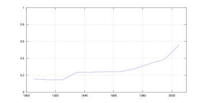
After trying out general proper noun phrases produced inconclusively noisy results, we decided to focus on occurrences of personal names, detected in the text by a proprietary state-of-the-art statistical recognizer. Personal names have a relatively stable presence in the media: even with high OCR error rates in old microform, over 1/7th of the articles even in the earliest decades since 1900 contain recognized personal names (see Figure 2).
But personal names are not without historical caveats, either. A woman appearing in 2005 stories as “Jane Smith” would be much more likely to be exclusively referenced as “Mrs. Smith”, or even “Mrs. John Smith”, in 1915. Also, the English-speaking world was much more Anglo-centric in 1900 than now, with much less diversity of names. An informal sample suggests that most names with non-trivial news presence 100 years ago referred overwhelmingly to a single bearer of that name for the duration of a particular news topic, but many names are not unique when taken across the duration of the whole corpus — for instance, “John Jacob Astor”, appearing in the news heavily over several decades (Fig. 3), in reference to a number of distinct relatives. On account of both of these phenomena, among others, we aim to focus on name appearance patterns that are most likely to represent a single news story or contiguous span of public attention involving that person, rather than trying to model the full media “lifetime” of individuals, as we had considered doing at the start of this project.
2.1.4 OCR errors in data and metadata
We empirically discovered another downfall of studying long-term “media lifetimes” of individuals. In an early experiment, we measured, for each personal name, the 10th and 90th percentiles of the dates of that name’s occurrence in the news. We then looked at the time interval between 10th and 90th percentiles, postulating that a large enough fraction of names are unique among newsworthy individuals that the distribution of these inter-quantile gaps could be a robust measure of media lifetime. After noticing a solid fraction of the dataset showing inter-quantile gaps on the scale of 10-30 years, we examined a heat map of gap durations, and discovered a regular pattern of gap durations at exact-integer year offsets, which, other than for Santa Claus, Guy Fawkes, and a few other clear exceptions, seemed an improbable phenomenon.
This turned out to be an artifact of OCRed metadata. In particular, the culprit was single-digit OCR errors in the scanned article year. While year errors are relatively rare, every long-tail name that occurred in fewer than 10 articles (often within a day or two of each other), and had a mis-OCRed error for one of those occurrences contributed probability mass to integral-number-of-years media lifetimes. As extra evidence, the heat map had a distinct outlier segment of high probability mass for inter-quantile range of exactly 20 years, starting in the 1960s and ending in the 1980s — the digits 6 and 8 being particularly easy to mistake on blurry microfilm. Note that short-term phenomena are relatively safe from OCR date errors, thanks to the common English convention of written-out month names, and to the low impact of OCR errors in the day number.
OCR errors in the article text itself are ubiquitous. Conveniently, the edit distance between two recognizable personal names is rarely very short, so by agreeing to discard any name that occurs only once in the corpus, we are likely to discard virtually all OCR errors as well, with no impact on data on substantially newsworthy people. We should note that OCR errors are noticeably more frequent on older microfilm, but the reasonable availability of recognizable personal names even in 100-year-old articles, per Fig. 2, suggests that this problem is not dire. A manually-coded sample of 50 articles with recognized names from the first decade of the 1900s showed only 8 out of 50 articles having incorrectly recognized names (including both OCR errors and non-names mis-tagged as names).
2.1.5 Simultaneity and publishing cycles
There are also pitfalls with examining short timelines. In the earliest decades we examine, telegraph was widely available to news publishers, but not fully ubiquitous, with rural papers often reporting news “from the wire” several days after the event. An informal sample seems to suggest that most news by 1900 propagated across the world on the scale of a few days. Also, many publications in the corpus until the last 20 years or so were either published exclusively weekly or, in the case of Sunday newspaper issues, had substantially higher volume once a week, resulting in many otherwise obscure names having multiple news mentions separated by one week — a rather different phenomenon than a person remaining in the daily news for a full week. On account of both of these, we generally disregard news patterns that are shorter than a few days in our study design.
3 Measuring Fame
We begin by producing a list of names for each article. To do this, we extract short capitalized phrases from the body text of each article, and keep phrases recognized by an algorithm to be personal names.
For every name that appears in the input, we consider that name’s timeline, which is the multiset of dates at which that name appears, including multiple occurrences within an article. We intend the timeline to approximate the frequency with which a person browsing the news at random on a given day would encounter that name. The accuracy of this approximation will depend on the volume of news articles available. In order to avoid the possibility that any trends we detect are caused by variations in this accuracy caused by variations in the volume of the corpus, we randomly choose an approximately equal number of articles to work with from each month. We describe and analyze this process in Section 3.3.
In general, our method can be applied to any collection of timelines. In Section 5, we apply it to names extracted from blog posts.
3.1 Finding Periods of Fame
Once we have computed a timeline for each name that appears in the corpus, we select a time during which we consider that name to have had its period of fame, using one of the two methods described below. In order to compare the phenomenon of fame at different points in time, we consider the joint distribution of two variables over the set of names: the peak date and the duration of the name’s period of fame. We try the following two methods to compute a peak date and duration for each timeline.
-
•
Spike method. This method intends to capture the spike in public attention surrounding a particular news story. We divide time into one-week intervals and consider the name’s rate of occurrence in each interval. The week with the highest rate is considered to be the peak date, and the period extends backward and forward in time as long as the rate does not drop below one tenth its maximum rate. Yang and Leskovec [13] used a similar method in their study of digital media, using a time scale of hours where we use weeks.
-
•
Continuity method. This method intends to measure the duration of public interest in a person. We define a name’s period of popularity to be the longest span of time within which there is no seven-day period during which it is not mentioned. The peak date falls halfway between the beginning and the end of the period. We find, in Section 4, that durations are short compared to the time span of the study, so using any choice of peak date between the beginning and end will produce similar distributions.
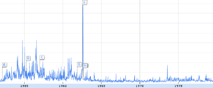
To demonstrate the distinction between these two methods, Figure 3 shows the occurrence timeline for Marilyn Monroe. The “continuity method” picks out the bulk of her fame — 1952-02-13 (“A”) through 1961-11-15 (“D”), by which point her appearance in the news was reduced to a fairly low background level. The “spike method” picks out the intense spike in interest surrounding her death, yielding the range 1962-7-18 (“E”) – 1962-8-29 (“H”).
Very often these two methods identify short moments of fame within a much longer context. For example, in Figure 3, we see the timeline for the name “John Jacob Astor”, normalized by article counts. The spike method identifies as the peak the death of John Jacob Astor III of the wealthy Astor family, with a duration of 38 days (March 8 to February 15, 1890). The continuity method identifies instead the death of his nephew John Jacob Astor IV, who died on the Titanic, with a period of five months [12]. The period begins on March 23, 1912, three weeks before the Titanic sank, and ends August 31. Many of the later occurrences of the name are historical mentions of the sinking of the Titanic.

3.2 Choosing the Set of Names
Basic filtering
In all our experiments, to reduce noise, we discard the names which occurred less than ten times, or whose fame durations are less than two days. (In both methods, a name whose fame begins Monday and ends Wednesday is considered to have a duration of two days.) We also remove peaks that end in 2011 or later, since these peaks might extend further if our news corpus extended further in the future.
Top 1000 by year
For each peak type, we repeat our experiment with the set of names restricted in the following way. We counted the total number of times each name appeared in each year (counting repeats within an article). For each year, we produced the set of the 1000 most frequently mentioned names in that year. We took the union of these sets over all years, and ran our experiments using only the names in this set. Note that a name’s peak of popularity need not be the same year in which that name was in the top 1000: so if a name is included in the top-1000 set because it was popular in a certain year, we may yet consider that name’s peak date to be a different year.
Top 0.1% by year
We consider that filtering to the top 1000 names in each year might introduce the following undesirable bias. Suppose names are assigned peak durations according to some universal distribution, and later years have more names, perhaps because of the increasing volume of news. If a name’s frequency of occurrence is proportional to its duration, then selecting the top 1000 names in each year will tend to produce names with longer durations of fame in years with a greater number of names. With this in mind, we considered one more restriction on the set of names. In each year , we considered the total number of distinct names mentioned in that year. We then collected the top names in each year . We ran our experiments using only the names in the union of those sets. As with the top-1000 filtering, a name’s peak date will not necessarily be the same year for which it was in the top 0.1% of names.
3.3 Sampling for Uniform Coverage
The spike and continuity methods for identifying periods of fame may be affected by the volume of articles available in our corpus. For example, suppose a name’s timeline is generated stochastically, with every article between February 1 and March 31 containing the name with a 1% probability. If the corpus contains 10000 articles in every week, then both the spike and continuity methods will probably decide that the article’s duration is two months. However, if the corpus contains less than 100 articles in each week, then the durations will tend to be short, since there will be many weeks during which the name is not mentioned.
We propose a model for this effect. Each name has a “true” timeline which assigns to each day a probability that an article on that day will mention .444 In fact, articles could mention the name multiple times, but in the limit of a large number of articles, this will not affect our analysis. For each day, there is a total number of articles ; we have no knowledge of the relation between and , except that there is some lower bound for all within some reasonable range of time. Then we suppose the timeline for name is a sequence of independent random variables . Our goal is to ensure that any measurements we take are independent of the values .
To accomplish this independence of news volume, we randomly sampled news articles so that the expected number in each month was . Let be the number of sampled articles containing name . If we were to randomly sample articles without replacement, then we would have . Notice that the joint distribution of the random variables is unaffected by the article volumes . Any further measurement based on the variables will therefore also be unrelated to the sequence . In practice, instead of sampling exactly articles without replacement, we flipped a biased coin for each of the articles at time , including each article with probability . For a large enough volume of articles, the resulting measurements will be the same.
We removed all articles published before 1895, since the months before 1895 had less than our target number of articles. We also removed articles published after the end of the year 2010, to avoid having a month with news articles at the beginning but not the end of the month, but with the same number of sampled articles.
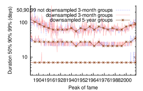
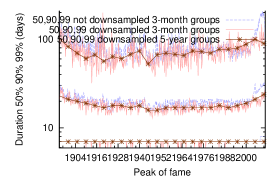
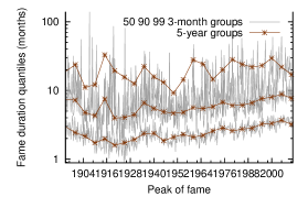
As an example of the effect of downsampling, the blue dotted lines in Figure 9 show the 50th, 90th and 99th percentiles of the distribution of fame durations using the continuity method. We see that they increase suddenly in the last ten years, when our coverage of articles surges with the digital age. The red lines show the same measurement after downsampling: the surge no longer appears.
3.4 Graphing the Distributions
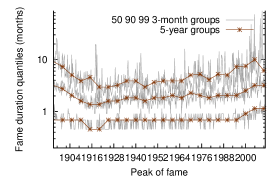
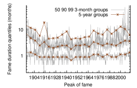
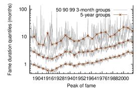
We graph the joint distribution of peak dates and durations in two different ways. We consider the set of names which peak in successive five-year periods. Among each set of names, we graph the 50th, 90th and 99th percentile durations of fame. These appear as darker lines in the graphs; for example, the top of Fig. 6 shows the distribution for the spike method. The lighter solid red lines show the same three quantiles for shorter three-month periods. For comparison, the dashed light blue lines show the same results if the article sampling described in Sec. 3.3 is not performed (and articles before 1895 and after 2010 are not removed). Fig. 9 shows the same set of lines using the continuity method. All the later figures are produced in the same way, except they do not include the non-sampled full distributions.
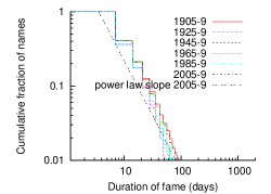
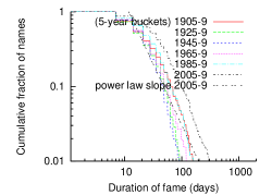
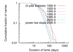
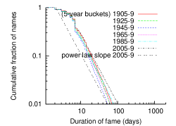
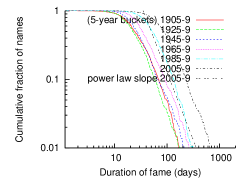
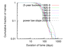
The second type of graph focuses on one five-year period at a time. The bottom of Fig. 6 shows a cumulative plot showing the number of names with duration greater than that shown on the -axis. This is plotted for many five-year periods. The graphs of measurements using the spike method look more like step functions because that method measures durations in seven-day increments, whereas the longest-stretch method can yield any number of days. (Recall that peaks that last less than two days are removed.)
3.5 Estimating Power Law Exponents
We test the hypothesis that the tail of the distribution of fame durations follows a power law. For a given five-year period, we collect all names which peak in that period, and consider 20% of the names with the longest fame durations – that is, we set to be the 80th percentile of durations, and consider durations . Among those 20%, we compute a maximum likelihood estimate of the power law exponent , predicting that the probability of a duration is . Clauset et al [3] show that the maximum likelihood estimate is given by . We include a line on each plot of cumulative distributions of fame durations, of slope on the log-log graph because we plot cumulative distributions rather than density functions. The values we measure are discussed in the following sections, and summarized in Figure 4 for the news corpus and Figure 5 for the blog corpus.
3.6 Statistical Measurements
We used bootstrapping to estimate the uncertainty in the four statistics we measured: the 50th, 90th and 99th percentile durations and of the best-fit power law exponents. For selected five-year periods, we sampled names with replacement from the set of names that peaked in that period of time. For each statistic, we repeated this process 25000 times, and reported the range of numbers within which 99% of our samples fell. The results are presented in Figures 4 (for the news corpus) and 5 (for the blog corpus).
| method | filtering | period | 50th %ile (days) | 90th %ile (days) | 99th %ile (days) | power law exponent |
|---|---|---|---|---|---|---|
| spike | all | 1905-9 | 7 (7 .. 7) | 28 (28 .. 28) | 91 (78 .. 106) | -2.45 (-2.55 .. -2.21) |
| spike | all | 1925-9 | 7 (7 .. 7) | 28 (28 .. 28) | 65 (63 .. 78) | -2.63 (-2.74 .. -2.33) |
| spike | all | 1945-9 | 7 (7 .. 7) | 21 (21 .. 28) | 56 (49 .. 63) | -2.44 (-2.50 .. -2.38) |
| spike | all | 1965-9 | 7 (7 .. 7) | 21 (21 .. 28) | 63 (56 .. 70) | -2.37 (-2.44 .. -2.31) |
| spike | all | 1985-9 | 7 (7 .. 7) | 21 (21 .. 28) | 70 (63 .. 78) | -2.32 (-2.36 .. -2.27) |
| spike | all | 2005-9 | 7 (7 .. 7) | 28 (28 .. 28) | 84 (78 .. 91) | -2.48 (-2.53 .. -2.43) |
| spike | top 1000 | 1905-9 | 21 (21 .. 21) | 63 (56 .. 70) | 155 (133 .. 192) | -2.75 (-3.15 .. -2.56) |
| spike | top 1000 | 1925-9 | 21 (14 .. 21) | 49 (46 .. 56) | 91 (78 .. 113) | -3.22 (-3.74 .. -2.99) |
| spike | top 1000 | 1945-9 | 21 (14 .. 21) | 49 (42 .. 49) | 91 (70 .. 130) | -3.33 (-3.73 .. -2.89) |
| spike | top 1000 | 1965-9 | 21 (21 .. 21) | 56 (49 .. 63) | 119 (99 .. 164) | -2.90 (-3.54 .. -2.65) |
| spike | top 1000 | 1985-9 | 21 (21 .. 28) | 63 (56 .. 78) | 161 (121 .. 366) | -2.85 (-3.19 .. -2.57) |
| spike | top 1000 | 2005-9 | 35 (28 .. 35) | 99 (84 .. 119) | 309 (224 .. 439) | -2.64 (-2.96 .. -2.44) |
| spike | top 0.1% | 1905-9 | 35 (28 .. 42) | 122 (91 .. 155) | 289 (161 .. 381) | -2.82 (-3.96 .. -2.36) |
| spike | top 0.1% | 1925-9 | 28 (21 .. 35) | 63 (56 .. 82) | 145 (91 .. 218) | -3.49 (-4.82 .. -2.92) |
| spike | top 0.1% | 1945-9 | 21 (21 .. 28) | 56 (49 .. 67) | 133 (84 .. 161) | -3.35 (-4.32 .. -2.78) |
| spike | top 0.1% | 1965-9 | 28 (21 .. 35) | 70 (63 .. 99) | 162 (119 .. 494) | -2.90 (-3.77 .. -2.47) |
| spike | top 0.1% | 1985-9 | 35 (28 .. 35) | 90 (70 .. 113) | 327 (140 .. 443) | -2.66 (-3.13 .. -2.35) |
| spike | top 0.1% | 2005-9 | 35 (35 .. 42) | 119 (99 .. 140) | 338 (263 .. 557) | -2.76 (-3.10 .. -2.44) |
| continuity | all | 1905-9 | 7 (7 .. 7) | 20 (19 .. 21) | 70 (64 .. 79) | -2.67 (-2.76 .. -2.59) |
| continuity | all | 1925-9 | 7 (7 .. 7) | 18 (17 .. 19) | 64 (56 .. 71) | -2.64 (-2.72 .. -2.53) |
| continuity | all | 1945-9 | 7 (7 .. 7) | 16 (15 .. 16) | 53 (49 .. 58) | -2.74 (-2.82 .. -2.66) |
| continuity | all | 1965-9 | 7 (7 .. 7) | 17 (16 .. 18) | 66 (58 .. 75) | -2.58 (-2.69 .. -2.52) |
| continuity | all | 1985-9 | 7 (7 .. 7) | 18 (17 .. 18) | 77 (71 .. 83) | -2.48 (-2.56 .. -2.44) |
| continuity | all | 2005-9 | 7 (7 .. 7) | 21 (20 .. 21) | 101 (96 .. 108) | -2.43 (-2.46 .. -2.40) |
| continuity | top 1000 | 1905-9 | 24 (23 .. 26) | 69 (62 .. 76) | 166 (136 .. 229) | -3.01 (-3.35 .. -2.70) |
| continuity | top 1000 | 1925-9 | 22 (21 .. 24) | 58 (53 .. 66) | 176 (131 .. 338) | -3.01 (-3.39 .. -2.67) |
| continuity | top 1000 | 1945-9 | 27 (25 .. 29) | 66 (57 .. 80) | 211 (169 .. 332) | -2.92 (-3.32 .. -2.59) |
| continuity | top 1000 | 1965-9 | 34 (32 .. 35) | 92 (81 .. 104) | 262 (203 .. 622) | -2.75 (-3.11 .. -2.48) |
| continuity | top 1000 | 1985-9 | 52 (49 .. 56) | 135 (118 .. 147) | 312 (231 .. 739) | -3.20 (-3.62 .. -2.83) |
| continuity | top 1000 | 2005-9 | 87 (80 .. 91) | 229 (211 .. 250) | 649 (532 .. 752) | -2.97 (-3.32 .. -2.75) |
| continuity | top 0.1% | 1905-9 | 66 (59 .. 79) | 146 (126 .. 176) | 968 (209 .. 4287) | -3.29 (-5.20 .. -2.24) |
| continuity | top 0.1% | 1925-9 | 53 (47 .. 61) | 125 (104 .. 161) | 476 (258 .. 2498) | -2.67 (-3.72 .. -2.20) |
| continuity | top 0.1% | 1945-9 | 57 (52 .. 66) | 150 (123 .. 194) | 419 (218 .. 1089) | -3.19 (-4.26 .. -2.52) |
| continuity | top 0.1% | 1965-9 | 69 (61 .. 79) | 168 (143 .. 214) | 713 (261 .. 874) | -3.01 (-4.01 .. -2.45) |
| continuity | top 0.1% | 1985-9 | 85 (78 .. 94) | 187 (158 .. 216) | 732 (276 .. 892) | -3.40 (-4.30 .. -2.80) |
| continuity | top 0.1% | 2005-9 | 113 (107 .. 119) | 271 (246 .. 306) | 681 (614 .. 874) | -3.16 (-3.59 .. -2.85) |
| method | filtering | period | 50th %ile (days) | 90th %ile (days) | 99th %ile (days) | power law exponent |
|---|---|---|---|---|---|---|
| spike | all | 2000-4 | 7 (7 .. 7) | 35 (28 .. 35) | 123 (84 .. 189) | -2.37 (-2.52 .. -2.23) |
| spike | all | 2005-9 | 7 (7 .. 7) | 28 (21 .. 28) | 75 (63 .. 84) | -2.34 (-2.76 .. -2.27) |
| spike | top 1000 | 2000-4 | 21 (14 .. 21) | 56 (49 .. 63) | 265 (148 .. 479) | -2.51 (-2.83 .. -2.18) |
| spike | top 1000 | 2005-9 | 14 (14 .. 21) | 49 (42 .. 54) | 109 (91 .. 151) | -2.74 (-3.03 .. -2.41) |
| spike | top 0.1% | 2000-4 | 39 (28 .. 56) | 189 (106 .. 305) | 717 (286 .. 840) | -2.26 (-3.05 .. -1.85) |
| spike | top 0.1% | 2005-9 | 28 (25 .. 35) | 88 (74 .. 102) | 213 (113 .. 1674) | -3.29 (-5.40 .. -2.23) |
| continuity | all | 2000-4 | 7 (7 .. 7) | 22 (20 .. 23) | 114 (95 .. 160) | -2.38 (-2.49 .. -2.28) |
| continuity | all | 2005-9 | 6 (6 .. 7) | 18 (17 .. 19) | 80 (66 .. 93) | -2.62 (-2.72 .. -2.53) |
| continuity | top 1000 | 2000-4 | 20 (18 .. 21) | 71 (59 .. 83) | 387 (237 .. 819) | -2.32 (-2.54 .. -2.12) |
| continuity | top 1000 | 2005-9 | 21 (20 .. 22) | 59 (53 .. 73) | 408 (211 .. 1057) | -2.37 (-2.62 .. -2.18) |
| continuity | top 0.1% | 2000-4 | 102 (89 .. 123) | 372 (236 .. 768) | 2010 (768 .. 2238) | -2.24 (-3.15 .. -1.86) |
| continuity | top 0.1% | 2005-9 | 83 (70 .. 93) | 302 (193 .. 617) | 2083 (954 .. 2991) | -2.12 (-2.75 .. -1.79) |
4 Results: News Corpus
We measure periods of popularity using the spike and continuity methods described in Section 3, and in each case plot the distribution of duration as it changes over time.
Figures 6 and 9 show the evolution of the distribution of fame durations for the full set of names in the corpus (after the basic filtering described in Section 3.2) using the spike and continuity methods, respectively. (Section 3.4 describes the format of the graphs in detail.)
Median durations
For the entire period we studied, the median fame duration did not decrease, as we had expected, but rather remained completely constant at exactly 7 days, for both the spike and the continuity peak measurement methods. For the spike method alone, this would not have been surprising. Peaks measured by the spike method are discretized to multiples of weeks, so a perennial median of 7 days just shows that multi-week durations have never been common. On the other hand, the continuity method freely admits fame durations in increments of 1 day, with only 1-day-long peaks filtered out. Yet, the median has remained at exactly 7 days for all the years studied, and, per the full-corpus “50th percentile” measurements, shown in blue in Figure 4, for all decades where we’ve tried bootstrapping, 99% of bootstrapped samples also matched the 7-day measurement exactly (for the continuity method and, less surprisingly, for the spike method). This gives strong statistical significance to the claim that 7 days is indeed a very robust measurement of typical fame duration, which has not varied in a century.
The most famous
We next consider specially the fame durations of the most famous names, in two correlated, but distinct senses of “most famous”:
-
•
“Duration outliers” — people whose fame lasts much longer than typical, as measured by the 90th and 99th percentiles of fame durations within each year. These correspond to the top two lines in the timelines of Figures 6 and 9, and the columns “90 %ile” and “99 %ile” of the first and fourth blocks of Figure 4.
-
•
“Volume outliers” – the names which appear the most frequently in the news, by being either in the top 1000 most frequent names in some year, or, separately, names in the top 0.1%, as per Section 3.2. The graphs for these subsets of names are shown in Figures 7 and 8 for the spike method, and Figures 10 and 11 for the continuity method, and the statistical measurements appear in blocks 2, 3, 5 and 6 of Figure 4.
From the 1900’s to the 1940’s, the fame durations in both categories of outliers do tend to decrease, with the decreases across that time interval statistically signicantly lower-bounded by 1-2 weeks via 99% bootstrapping intervals. Heuristically, this seems consistent with our original hypothesis that accelerating communications shorten fame durations: 1-2 weeks is a reasonable delay to be incurred by sheer communications delay before the omnipresence of telegraphy and telephony. We note with curiosity that this effect applies only to the highly-famous outliers rather than the typical fame durations. We posit that this is perhaps due to median fame durations being typically attributable to people with only geographically localized fame, which does not get affected by long communication delays. We leave to further work a more nuanced study to test these hypotheses around locality and communication delays affecting news spread in the early 20th century.
After the 1940’s, on the other hand, we see no such decrease. On the contrary, the durations of fame for both the duration outliers and the volume outliers reverse the trend, and actually begin to slowly increase. Using the bootstrapping method, per Section 3.6, we get the results marked in red in Figure 4: in almost all of the outlier studies5557 out of the 8 outlier studies show statistically significant increases between the 1940’s and the 1980’s, and between the 1960’s and the 2000’s. The sole exception is the 90th percentile of the spike method. Given that the bootstrap values in that experiment, discretized to whole weeks, range between 3 and 4 weeks, we don’t consider it surprising that the increases there were not measured to be significant by 99% bootstrap intervals., we see that the increase in durations is statistically significant over 40-year gaps for both categories of fame outliers. For example, the median fame duration according to continuity peaks for the top 1000 names (50th percentile column of the fifth block) appears as “27 (25 .. 29)” in the period 1945-9 and “52 (49 .. 56)” for the period 1985-9: with 99% confidence, the median duration was less than 29 days in the former period, but greater than 49 days in the latter.
We also ran experiments for names that have outlier durations within the subset of names with outlier volumes. The same general trends were seen there as with the above outlier studies, but, with a far shallower pool of data, the bootstrapping-based error bars were generally large enough to not paint a convincing, statistically significant picture.
Power law fits
The column titled “power law exponent” in Figure 4 shows the maximum likelihood estimates of the power law exponents for various five-year-long peak periods. We focus on the first and fourth blocks, which show the estimates for the full set of names for the spike method and the continuity method respectively.
For both peak methods, the fitted power law exponents remain in fairly small ranges — between -2.77 and -2.45 for continuity peaks, and between -2.63 and -2.32 for spike peaks. In Figures 9 and 6 we show the actual distributions, and, for reference, comparisons with the power-law fit for the 2005-2009 data (a straight line on these log-log plots).
Furthermore, the continuity peaks fits also support the above observation of slowly-growing long-tail fame durations from 1940 onward. That is, power-law exponents from 1940 onward slowly move toward zero, with statistically significant changes when compared at 40-year intervals. The fluctuations and the error bars for both methods are rather noticeable, though, suggesting that power laws make for only a mediocre fit to this data.
5 Results: Blog Posts
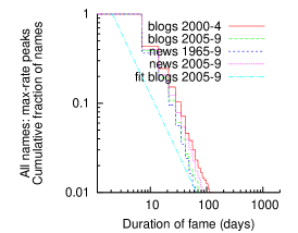
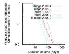
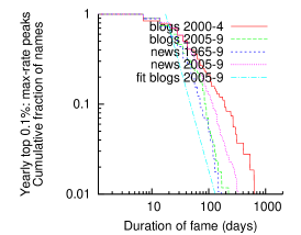
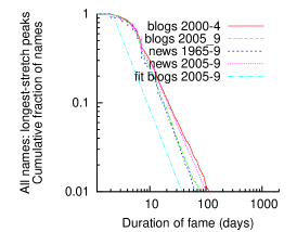
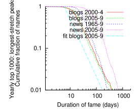
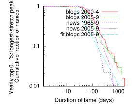
We also ran our experiments on a second set of data consisting of public English-language blog posts from the Blogger service. We began by sampling so that the number of blog posts in each month in our data set was equal to the number of news articles we sampled in each month, as per Sec. 3.3. The cumulative graphs of fame duration from six experiments are shown in Fig. 12. We combine the two methods for identifying periods of fame with three sets of names described in Section 3.2. The respective distributions from the news corpus are superimposed for comparison.
The graphs of fame duration measured using the continuity method are much smoother for the blog corpus than for the news corpus. This happens because whereas we only know which day each news article was written, we know the time of day each blog entry was posted.
The continuity-method graphs (bottom of Figure 12) had a distinctive rounded cap which surprised us at first. We believe it is caused by the following effect. Peaks with only two mentions in them are fairly common, and have a simple distinctive distribution that is the difference between two sample dates conditioned on being less than a week apart. Since two dates that are longer than one week apart cannot constitute a longest-stretch peak, the portion of the graph with durations longer than one week does not include any names from this two-sample distribution, and so it looks different. Our estimates of power-law exponents only consider the longest 20% of durations, so they ignore this part of the graph.
The estimates we computed for the power-law exponents of the duration distributions for blog data are shown in Figure 5, and can be compared to the figures for news articles in Figure 4.
The medians for both blogs and news for both methods are remarkably the same, with no statistically significant differences. The power law fits are also quite similar, although they show enough variation to produce statistically significant differences. Qualitatively, we take these as evidence that the fame distributions in news and blogs are coarsely similar, and that it is not unreasonable to consider these results as casting some light on more fundamental aspects of human attention to and interest in celebrities, rather than just on the quirks of the news business.
We do leave open the question of accounting for the occasionally significant distinctions between outlier results for blogs, as compared to news, especially for outlier-volume continuity peaks.
6 Related Work
Michel et al. [9] study a massive corpus of digitized content in an attempt to study cultural trends. The corpus they study is even larger than ours in terms of both volume and temporal extension.
Leetaru [7] presents evidence that sentiment analysis of news articles from the past decade could have been used to predict the revolutions in Tunisia, Egypt and Libya.
Our spike method for identifying periods of fame is motivated in part by the work of Yang and Lescovec [13] on identifying patterns of temporal variation on the web. Szabo and Huberman [11] also consider temporal patterns, in their case regarding consumption of particular content items. Kleinberg studies other approaches to identification of bursts [6].
Numerous works have studied the propagation of topics through online media. Leskovec et al. [8] develop techniques for tracking short “memes” as they propagate through online media, as a means to understanding the news cycle. Adar and Adamic [2], and Gruhl et al. [5] consider propagation of information across blogs.
Finally, a range of tools and systems provide access to personalized news information; see Gabrilovich et al [4] and the references therein for pointers.
7 Acknowledgements
The authors would like to thank Zoran Dimitrijevic and the Google News Archive team for their help with the data; Danny Wyatt, Ed Chi, and Rachel Schutt for statistical advice; and the anonymous reviewers for helpful suggestions.
References
- [1] Media landscape redefined by 24-second news cycle. The Onion, 2007-06-01. http://www.theonion.com/articles/media-landscape-redefined-by-24second-news-cycle,2213/.
- [2] E. Adar and L. A. Adamic. Tracking information epidemics in blogspace. WI 2005, pages 207–214.
- [3] A. Clauset, C. R. Shalizi, and M. E. J. Newman. Power-law distributions in empirical data. SIAM Review, 51(4):661–703, 2009.
- [4] E. Gabrilovich, S. Dumais, and E. Horvitz. Newsjunkie: providing personalized newsfeeds via analysis of information novelty. WWW 2004, pages 482–490.
- [5] D. Gruhl, R. Guha, D. Liben-Nowell, and A. Tomkins. Information diffusion through blogspace. WWW 2004, pages 491–501.
- [6] J. Kleinberg. Bursty and hierarchical structure in streams. KDD 2002, pages 91–101.
- [7] K. Leetaru. Culturomics 2.0: Forecasting large-scale human behavior using global news media tone in time and space. First Monday, 16(9-5), 2011.
- [8] J. Leskovec, L. Backstrom, and J. Kleinberg. Meme-tracking and the dynamics of the news cycle. KDD 2009, pages 497–506.
- [9] J-B. Michel, Y. K. Shen, A. P. Aiden, A. Veres, M. K. Gray, The Google Books Team, J. P. Pickett, D. Hoiberg, D. Clancy, P. Norvig, J. Orwant, S. Pinker, M. A. Nowak, and E. L. Aiden. Quantitative analysis of culture using millions of digitized books. Science, 331(6014):176–182, 2011.
- [10] H. A. Simon. Designing organizations for an information-rich world. 1971.
- [11] G. Szabo and B. A. Huberman. Predicting the popularity of online content. Commun. ACM, 53:80–88, August 2010.
- [12] Wikipedia. Astor family — Wikipedia, the free encyclopedia, 2011. [Online; accessed 10-August-2011].
- [13] J. Yang and J. Leskovec. Patterns of temporal variation in online media. WSDM 2011, pages 177–186.