Numerical evaluation of multi-loop integrals for arbitrary kinematics with SecDec 2.0

Abstract

We present the program SecDec 2.0 which contains various new features: First, it allows the numerical evaluation of multi-loop integrals with no restriction on the kinematics. Dimensionally regulated ultraviolet and infrared singularities are isolated via sector decomposition, while threshold singularities are handled by a deformation of the integration contour in the complex plane. As an application we present numerical results for various massive two-loop four-point diagrams. SecDec 2.0 also contains new useful features for the calculation of more general parameter integrals, related e.g. to phase space integrals.

PACS: 12.38.Bx, 02.60.Jh, 02.70.Wz

IPPP/12/22, DCPT/12/44, MPP-2012-75

, ,

PROGRAM SUMMARY

Numerical evaluation of multi-loop integrals for arbitrary kinematics with SecDec 2.0
Authors: S. Borowka, J. Carter, G. Heinrich
Program Title: SecDec 2.0
Journal Reference:
Catalogue identifier:
Licensing provisions: none
Programming language: Wolfram Mathematica, perl, Fortran/C++
Computer: from a single PC to a cluster, depending on the problem
Operating system: Unix, Linux
RAM: depending on the complexity of the problem
Keywords: Perturbation theory, Feynman diagrams, infrared and threshold singularities, numerical integration
PACS: 12.38.Bx, 02.60.Jh, 02.70.Wz
Classification:
4.4 Feynman diagrams, 5 Computer Algebra, 11.1 General, High Energy Physics and Computing.
Journal reference of previous version: Comput.Phys.Commun. 182 (2011) 1566-1581.

Nature of problem:
Extraction of ultraviolet and infrared singularities from parametric integrals appearing in higher order perturbative calculations in gauge theories. Numerical integration in the presence of integrable singularities (e.g. kinematic thresholds).

Solution method:
Algebraic extraction of singularities in dimensional regularisation using iterated sector decomposition. This leads to a Laurent series in the dimensional regularisation parameter $\epsilon$, where the coefficients are finite integrals over the unit-hypercube. Those integrals are evaluated numerically by Monte Carlo integration. The integrable singularities are handled by choosing a suitable integration contour in the complex plane, in an automated way.
Restrictions: Depending on the complexity of the problem, limited by memory and CPU time. The restriction that multi-scale integrals could only be evaluated at Euclidean points is superseded in version 2.0.

Running time:
Between a few minutes and several days, depending on the complexity of the problem.

1 Introduction

Currently we are in the fortunate situation of being confronted with a wealth of high energy collider physics data, enabling us to test our present understanding of fundamental interactions and to explore physics at the TeV scale. However, the accuracy which has been or will be reached by the experiments has to be matched by comparable precision in the theory predictions, and in most cases this means that calculations beyond the leading order in perturbation theory are necessary.

It is well known that in the calculation of higher order corrections, various types of singularities can arise at intermediate stages of the calculation. For example, loop integrals can contain ultraviolet (UV) as well as infrared (IR) singularites, phase space integrals over unresolved massless particles lead to infrared singularities, and there can be integrable singularities due to kinematic thresholds. The UV and IR singularities can be regularised by dimensional regularisation, such that they appear as poles in $1/\epsilon$, which cancel when the different parts of the calculation are combined to a physical observable. However, before such cancellations are possible, the $1/\epsilon$ poles have to be extracted. In the calculation of multi-loop integrals or real radiation at higher orders, this usually leads to the task of factorising the poles from complicated multi-parameter integrals. Sector decomposition [1, 2, 3] is a method to achieve such a factorisation. The program SecDec 1.0, presented in [4], performs this task in an automated way. Other public implementations of sector decomposition can be found in [5, 6, 7, 8], see also [9]. The method already has been applied in various calculations, listing all of them is beyond the scope of this paper, for a review see [10]. Here we just mention that there are also fruitful combinations of sector decomposition with other techniques, e.g. non-linear transformations [11], Mellin-Barnes and differential equation techniques [7, 12, 13], high-energy expansions [14, 15], or in the context of subtraction for unresolved double real radiation at NNLO [16, 17, 18, 19, 20, 21, 22, 23, 24]. A method developed over many years [25, 26, 27, 28, 29, 30] to calculate one- and two-loop integrals numerically in the physical region also partly uses sector decomposition, in combination with a careful analysis of the singularity structure of certain classes of integrals and the use of functional relations between loop integrands.

A limitation of the program SecDec 1.0 was the fact that the numerical integration of multi-scale integrals was only possible for Euclidean points, or, more precisely, values of the Mandelstam invariants and masses for which the denominator of the integrand is guaranteed to be of definite sign. For physical applications which go beyond one-scale problems, it is however crucial to be able to deal with integrable singularities, usually related to kinematic thresholds, in addition to the singularities in $\epsilon$. The program SecDec 2.0 is able to achieve this task, by an automated deformation of the integration contour into the complex plane. This allows the numerical calculation of multi-scale integrals in the physical region in an automated way. Non-planarity of the considered integral does not add any extra complications. Adding more mass scales also does not necessarily increase the complexity of the calculation with this method, as additional masses usually lead to a simpler IR singularity structure and therefore lead to less functions in the iterated decomposition. Therefore one can for instance obtain numerical results for two-loop integrals involving several mass scales where analytic methods reach their limit.

The method of contour deformation in a multi-dimensional parameter space in the context of perturbative calculations has been pioneered in [31] and later has been refined in various ways to be applied to calculations at one loop [32, 33, 34, 35, 36, 37, 38, 39] and at two loops [40, 41, 42, 43].
Another purely numerical method uses an extrapolation from large to small values of the (analytically infinitesimal) parameter moving the integration contour away from poles on the real axis [44, 45]. Numerical methods using dispersion relations, differential equations and/or numerical integration of Mellin-Barnes representations also have been worked out, see e.g. [46, 47, 48, 49, 50, 51, 52]. However, most numerical methods to calculate multi-scale integrals beyond one loop so far are either limited to specific types of integrals, or the parameters for the numerical integration have been carefully adapted to the individual integrals by the authors.

The aim of the work presented here is to provide a public program where the user can calculate multi-scale integrals without worrying too much about the details of the integrand. The singularity structure does not have to be known beforehand (but certainly the user has to make sure that, after the extraction of the poles regulated by dimensional regularisation, only integrable singularities remain). The program contains a sophisticated procedure to check and adjust the contour deformation parameters to optimize the convergence. For complicated integrals, the convergence can nonetheless depend critically on the settings for the numerical integration; therefore we also offer the possibility for the user to choose various parameters at the input level to tune the deformation.
We should note that, even though the functions which are produced after the factorisation of the singularites in $\epsilon$ are available in algebraic form, they are usually too complicated to be integrated analytically. Therefore the final integration is done by the Monte Carlo methods, meaning that the precision which can be achieved is limited, but in favour of a gain in general applicability. We also should remark that the method is applicable to any number of loops in principle, however memory problems in the algebraic part where the functions are generated, or bad numerical convergence can be expected if the complexity of the integral is very high.

The structure of this paper is as follows. In Section 2, we briefly describe the general framework. Section 3 gives an overview of the structure of the program and the new features introduced in SecDec version 2.0. Section 4 contains installation and usage instructions, while examples and results are presented in Section 5. A brief user manual is given in the Appendix. Detailed documentation is also coming with the code which is available at http://secdec.hepforge.org.

2 General framework

The procedure of factorising endpoint singularities from parameter integrals by iterated sector decomposition is described in [1, 4]. Here our main concern is the numerical integration for physical kinematics after the endpoint singularities have been extracted. Our method to do so is based on contour deformation, described in detail in Section 2.2. The following section serves to introduce some basic concepts.

2.1 Feynman integrals

We choose a scalar integral for ease of notation. Tensor integrals only lead to an additional function of the Feynman parameters and invariants in the numerator. For more details we refer to [4, 10].

A scalar Feynman integral $G$ in $D$ dimensions at $L$ loops with $N$ propagators, where the propagators can have arbitrary, not necessarily integer powers $\nu_{j}$, has the following representation in momentum space:

$$G = \int\prod\limits_{l=1}^{L}{\mathrm{d}}^{D}\kappa_{l}\;\frac{1}{\prod\limits_{j=1}^{N}P_{j}^{\nu_{j}}(\{k\},\{p\},m_{j}^{2})}$$

$${\mathrm{d}}^{D}\kappa_{l} = \frac{\mu^{4-D}}{i\pi^{\frac{D}{2}}}\,{\mathrm{d}}^{D}k_{l}\;,\;P_{j}(\{k\},\{p\},m_{j}^{2})=q_{j}^{2}-m_{j}^{2}+i\delta\;,$$ (1)

where the $q_{j}$ are linear combinations of external momenta $p_{i}$ and loop momenta $k_{l}$. Introducing Feynman parameters leads to

$$G = \frac{\Gamma(N_{\nu})}{\prod_{j=1}^{N}\Gamma(\nu_{j})}\int_{0}^{\infty}\,\prod\limits_{j=1}^{N}{\mathrm{d}}x_{j}\,\,x_{j}^{\nu_{j}-1}\,\delta\big{(}1-\sum_{i=1}^{N}x_{i}\big{)}\int{\mathrm{d}}^{D}\kappa_{1}\ldots{\mathrm{d}}^{D}\kappa_{L}$$

$$\left[\sum\limits_{i,j=1}^{L}k_{i}^{\rm{T}}\,M_{ij}\,k_{j}-2\sum\limits_{j=1}^{L}k_{j}^{\rm{T}}\cdot Q_{j}+J+i\,\delta\right]^{-N\nu}$$

$$= \frac{(-1)^{N_{\nu}}}{\prod_{j=1}^{N}\Gamma(\nu_{j})}\Gamma(N_{\nu}-LD/2)\int\limits_{0}^{\infty}\,\prod\limits_{j=1}^{N}dx_{j}\,\,x_{j}^{\nu_{j}-1}\,\delta(1-\sum_{l=1}^{N}x_{l})\frac{{\cal U}^{N_{\nu}-(L+1)D/2}}{{\cal F}^{N_{\nu}-LD/2}}$$

where

$${\cal F}(\vec{x}) = \det(M)\left[\sum\limits_{j,l=1}^{L}Q_{j}\,M^{-1}_{jl}\,Q_{l}-J-i\,\delta\right]$$ (2)

$${\cal U}(\vec{x}) = \det(M),\;N_{\nu}=\sum_{j=1}^{N}\nu_{j}\;.$$

The functions ${\cal U}$ and ${\cal F}$ also can be constructed from the topology of the corresponding Feynman graph [53, 54, 10], and the implementation of this construction in SecDec 2.0 is one of the new features of the program.

For a diagram with massless propagators, none of the Feynman parameters occurs quadratically in the function ${\cal F}={\cal F}_{0}$ . If massive internal lines are present, ${\cal F}$ gets an additional term ${\cal F}(\vec{x})={\cal F}_{0}(\vec{x})+{\cal U}(\vec{x})\sum\limits_{j=1}^{N}x_{j}m_{j}^{2}$.

${\cal U}$ is a positive semi-definite function. A vanishing ${\cal U}$ function is related to the UV subdivergences of the graph. Overall UV divergences, if present, will always be contained in the prefactor $\Gamma(N_{\nu}-m-LD/2)$. In the region where all invariants formed from external momenta are negative, which we will call the Euclidean region in the following, ${\cal F}$ is also a positive semi-definite function of the Feynman parameters $x_{j}$. Its vanishing does not necessarily lead to an IR singularity. Only if some of the invariants are zero, for example if some of the external momenta are light-like, the vanishing of ${\cal F}$ may induce an IR divergence. Thus it depends on the kinematics and not only on the topology (like in the UV case) whether a zero of ${\cal F}$ leads to a divergence or not. The necessary (but not sufficient) conditions for a divergence are given by the Landau equations [55, 56, 57]:

$$x_{j}\,(q_{j}^{2}-m_{j}^{2})=0\quad\forall\,j$$ (3)

$$\frac{\partial}{\partial k^{\mu}}\sum_{j}x_{j}\,\left(q_{j}^{2}(k,p)-m_{j}^{2}\right)=0\;.$$ (4)

If all kinematic invariants formed by external momenta are negative, the necessary condition ${\cal F}=0$ for an IR divergence can only be fulfilled if some of the parameters $x_{i}$ go to zero. These endpoint singularities can be regulated by dimensional regularisation and factored out of the function ${\cal F}$ using sector decomposition. The same holds for dimensionally regulated UV singularities contained in ${\cal U}$. However, after the UV and IR singularities have been extracted as poles in 1/$\epsilon$, for non-Euclidean kinematics we are still faced with integrable singularities related to kinematic thresholds. How we deal with these singularities will be described in the following section.

2.2 Deformation of the integration contour

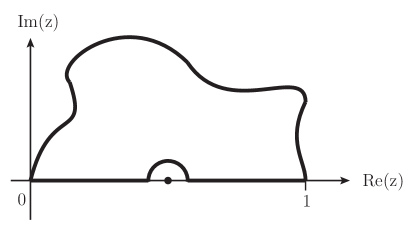
Figure 1: Schematic picture of the closed contour avoiding poles on the real axis.

Unless the function ${\cal F}$ in eq. (2) is of definite sign for all possible values of invariants and Feynman parameters, the denominator of a multi-loop integral will vanish within the integration region on a hypersurface given by the solutions of the Landau equations. If eq. (3) has a solution where $x_{j}>0\,\forall\,j$, all particles in the loop go simultaneously on-shell. This corresponds to a leading Landau singularity, which is not integrable (for real values of masses and momenta). However, the integrand can also diverge for certain values of kinematical invariants and Feynman parameters which represent a subleading Landau singularity, corresponding to an integrable singularity of logarithmic or squareroot type, related to normal thresholds. In these cases, we can make use of Cauchy’s theorem to avoid the non-physical poles on the real axis by a deformation of the integration contour into the complex plane. As long as the deformation is in accordance with the causal $i\delta$ prescription of the Feynman propagators, and no poles are crossed while changing the integration path, the integration contour can be changed such that the convergence of the numerical integration is assured. Using the fact that the integral over the closed contour in Fig. 1 is zero, we have

$$\int_{0}^{1}\prod\limits_{j=1}^{N}{\mathrm{d}}x_{j}{\cal I}(\vec{x})=\int_{0}^{1}\prod\limits_{j=1}^{N}{\mathrm{d}}x_{j}\left|\left(\frac{\partial z_{k}(\vec{x})}{\partial x_{l}}\right)\right|{\cal I}(\vec{z}(\vec{x}))\;,$$ (5)

where the $x_{i}$ are real, while $z_{i}$ are complex, describing a path parametrized by the variables $x_{i}$. The $i\delta$ prescription for the Feynman propagators tells us that the contour deformation into the complex plane should be such that the imaginary part of ${\cal F}$ should always be negative. For real masses and Mandelstam invariants $s_{ij}$, the following Ansatz [31, 33, 34] is therefore convenient:

$$\vec{z}(\vec{x}) =\vec{x}-i\;\vec{\tau}(\vec{x})$$

$$\tau_{k} =\lambda\,x_{k}(1-x_{k})\,\frac{\partial{\cal F}(\vec{x})}{\partial x_{k}}\;.$$ (6)

The derivative of ${\cal F}$ in eq. (2.2) is smallest in the extrema and largest where the slope is maximal. Hence, unless we are faced with a leading Landau singularity where both ${\cal F}$ and its derivatives with respect to $x_{i}$ vanish, the deformation leads to a well behaved integral at the points where the function ${\cal F}$ vanishes. A closed integration contour is guaranteed by the factors $x_{k}$ and $(1-x_{k})$, keeping the endpoints fixed. In terms of the new variables, we thus obtain

$${\cal F}(\vec{z}(\vec{x}))={\cal F}(\vec{x})-i\,\lambda\,\sum\limits_{j}\,x_{j}(1-x_{j})\,\left(\frac{\partial{\cal F}}{\partial x_{j}}\right)^{2}+{\cal O}(\lambda^{2})\;,$$ (7)

such that ${\cal F}$ acquires a negative imaginary part of order $\lambda$. Hence, the size of $\lambda$ determines the scale of the deformation. More technical details about the deformation are given in Section 3.3.

2.3 Parameter integrals

The program SecDec can also factorise singularities from parameter integrals which are more general than the ones related to multi-loop integrals. The only restrictions are that the integration domain should be the unit hypercube, and the singularities should be only endpoint singularities, i.e. should be located at zero or one. Contour deformation is not available in the subdirectory general, because the sign of the imaginary part telling us how to deform the contour is not fixed a priori for general functions, in contrast to loop integrals. However, we plan to implement the use of Cauchy’s theorem where applicable in a future version. Currently we assume that the singularities are regulated by non-integer powers of the integration parameters, where the non-integer part is the $\epsilon$ of dimensional regularisation or some other regulator. The general form of the integrals is

$$I=\int_{0}^{1}dx_{1}\ldots\int_{0}^{1}dx_{N}\prod_{i=1}^{m}P_{i}(\vec{x},\{\alpha\})^{\nu_{i}}\;,$$ (8)

where $P_{i}(\vec{x},\{\alpha\})$ are polynomial functions of the parameters $x_{j}$, which can also contain some symbolic constants $\{\alpha\}$. The user can leave the parameters $\{\alpha\}$ symbolic during the decomposition, specifying numerical values only for the numerical integration step. This way the decomposition and subtraction steps do not have to be redone if the values for the constants are changed. The $\nu_{i}$ are powers of the form $\nu_{i}=a_{i}+b_{i}\epsilon$ (with $a_{i}$ such that the integral is convergent). Note that half integer powers are also possible.

3 The SecDec program

3.1 Structure

The program consists of two parts, an algebraic part and a numerical part. The algebraic part uses code written in Mathematica [58] and does the decomposition into sectors, the subtraction of the singularities, the expansion in $\epsilon$ and the generation of the files necessary for the numerical integration. In the numerical part, Fortran or C++ functions forming the coefficient of each term in the Laurent series in $\epsilon$ are integrated using the Monte Carlo integration programs contained in the Cuba library [59, 60], or Bases [61]. The different subtasks are handled by perl scripts. The flowchart of the program is shown in Fig. 2 for the basic building blocks to calculate multi-loop integrals. To calculate parameter integrals which are not necessarily related to loop integrals, the structure is the same except that contour deformation is not available. For more details about the features in the part general we refer to [4].

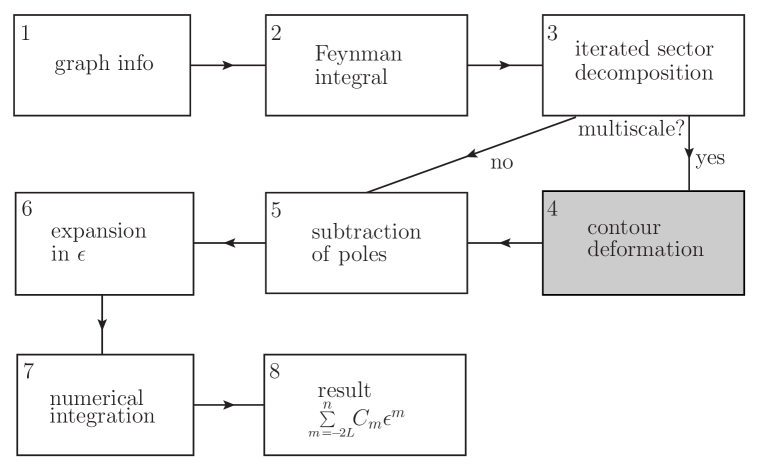
Figure 2: Flowchart showing the main steps the program performs to produce the result as a Laurent series in $\epsilon$.

The directories loop and general have the same global structure, only some of the individual files are specific to loop integrals or to more general parametric functions. The directories contain a number of perl scripts steering the decomposition and the numerical integration. The scripts use perl modules contained in the subdirectory perlsrc.

The Mathematica source files are located in the subdirectories src/deco (files used for the decomposition), src/subexp (files used for the pole subtraction and expansion in $\epsilon$) and src/util (miscellaneous useful functions). The documentation, created by robodoc [62] is contained in the subdirectory doc. It contains an index to look up documentation of the source code in html format by loading masterindex.html into a browser.

In order to use the program, the user only has to edit the following two files:

• param.input: (text file)
  specification of paths, type of integrand, order in $\epsilon$, output format, parameters for numerical integration, further options

• Template.m: (Mathematica syntax)

  • for loop integrals: specification of loop momenta and propagators, resp. of the topology; optionally numerator, non-standard propagator powers, space-time dimensions

  • for general functions: specification of integration variables, integrand, variables to be split

The program comes with example input and template files in the subdirectories loop/demos respectively general/demos, described in detail in [4].

3.2 New features of the program

Version 2.0 of SecDec contains the following new features, which will be described in detail in this section, while examples will be given in Section 5.

• loop part:

  • Multi-scale loop integrals can be evaluated without restricting the kinematics to the Euclidean region. This has been achieved by performing a (numerical) contour integration in the complex plane. The program automatically tries to find an optimal deformation of the integration path.

  • For scalar multi-loop integrals, the integrand can be constructed from the topological cuts of the diagram. The user only has to provide the vertices and the propagator masses, but does not have to provide the momentum flow.

  • The files for the numerical integration of multi-scale loop diagrams with contour deformation are written in C++ rather than Fortran. For integrations in Euclidean space, both the Fortran and the C++-versions are supported. The choice between Fortran and C++ can be made by the user in the param.input file by choosing either language=Cpp (default) or language=fortran .

  • A parallelisation of the algebraic part for Mathematica versions 7 and higher is possible if several cores are available.

  • The most recent version of the Cuba library, Cuba-3.0 (beta), is added to the program and used by default. The older version Cuba-2.1 is still supported.

  • The rescaling of the kinematic invariants is now possible by choosing rescale=1 (default is 0).

• general part:

  • The user can define additional (finite) functions at a symbolic level and specify them only later after the integrand has been transformed into a set of finite parameter integrals for each order in $\epsilon$.

• both parts:

  • The possibility to loop over ranges of parameter values is automated.

In the following we describe the new features in more detail.

3.3 Multi-scale loop integrals: Implementation of the contour deformation

As explained in Section 2.2, singularities on the real axis can be avoided by a deformation of the integration contour into the complex plane. The overall size of the deformation is controlled by the parameter $\lambda$ defined in eq. (2.2).

The convergence of the numerical integration can be improved significantly by choosing an “optimal” value for $\lambda$. Values of $\lambda$ which are too small lead to contours which are too close to the poles on the real axis and therefore lead to bad convergence. Too large values of $\lambda$ can modify the real part of the function to an unacceptable extent and could even change the sign of the imaginary part if the terms of order $\lambda^{3}$ get larger than the terms linear in $\lambda$. This would lead to a wrong result. Therefore we implemented a four-step procedure to optimize the value of $\lambda$, consisting of

• ratio check: To make sure that the terms of order $\lambda^{3}$ in eq. (7) do not spoil the sign of the imaginary part, we evaluate the ratio of the terms linear and cubic in $\lambda$ for a quasi-randomly chosen set of sample points to determine the maximal allowed $\lambda=\lambda_{max}$.

• modulus check: The imaginary part is vital at the points where the real part of ${\cal F}$ is vanishing. In these regions, the deformation should be large enough to avoid large numerical fluctuations due to a highly peaked integrand. Therefore we check the modulus of each subsector function ${\cal F}_{i}$ at a number of sample points, and pick the fraction of the value of $\lambda_{max}$ which maximises the minimum of the modulus of ${\cal F}_{i}$, i.e. the value of lambda which keeps ${\mathcal{F}}_{i}$ furthest from zero.

• individual $\lambda(i,j)$ adjustments: If the values of $\frac{\partial{\cal F}_{i}}{\partial x_{j}}$ are very different in magnitude, it can be convenient to have an individual parameter $\lambda(i,j)$ for each subsector function ${\cal F}_{i}$ and each Feynman parameter $x_{j}$.

• sign check: After the above adjustments to $\lambda$ have been made, the sign of Im$(\mathcal{F})$ is again checked for a number of sample points. If the sign is ever positive, this value of $\lambda$ is disallowed.

The contour deformation can be switched on or off by choosing
contourdef=True/False in the input file param.input. Obviously, the calculation takes longer if contour deformation is done, so if the integrand is known to be positive definite, contour deformation should be switched off. We also should emphasize that for integrands with a complicated threshold structure, the success of the numerical integration can critically depend on the parameters which tune the deformation, and on the settings for the Monte Carlo integration. In order to allow the user to tune the deformation, the following parameters can be adjusted by the user in the input file:

lambda:

the program takes the $\lambda$ value given in param.input as a starting point. If, after the program has performed the checks listed above, this $\lambda$ is found to be unsuitable or suboptimal, the value of $\lambda$ will be changed automatically by the program. The default is lambda=1.0.

largedefs:

If the integrand is expected to have (integrable) endpoint singularities at $x_{j}=0$ or 1, the deformation should be large in order to move the contour away from the problematic region. If largedefs=1 (default is 0), the program tries to enlarge the deformation at the endpoints.

smalldefs:

If the integrand is expected to be oscillatory and hence sensitive to small changes in the deformation parameter $\lambda$, choosing the flag smalldefs=1 (default is 0) will minimize the argument of each subsector function ${\cal F}_{i}$ by varying $\lambda(i,j)$.

3.4 Topology-based construction of the integrand

As already mentioned in section 2, the functions ${\cal U}$ and ${\cal F}$ can be constructed from the topology of the corresponding Feynman graph [53, 54, 10], without the need to assign the momenta for each propagator explicitly. The user only has to label the external momenta and the vertices. If an external momentum $p_{i}$ is part of a vertex, this vertex needs to carry the label $i$. The labelling of vertices containing only internal lines is arbitrary. In Template.m, the user has to specify proplist as a list of entries of the form $\{ms[k],\{i,j\}\}$, where $ms[k]$ is the mass squared of the propagator connecting vertex $i$ and vertex $j$. The mass label $k$ must correspond the the $k$th entry of the list of masses given in param.input. While $k$ needs to be the number labelling the masses, $ms[k]$ (with $k$ being an integer) can be left symbolic during the decomposition. However, if the mass is zero, one has to put $\{0,\{i,j\}\}$, because this changes the singularity structure at decomposition level.

An example is given below, more examples can be found in the mathematica template files templateP126.m, templateBnp6*.m, templateJapNP.m, templateggtt*.m in the subdirectory loop/demos. This feature of constructing the graph topologically is only implemented for scalar integrals so far. The original form of specifying the propagators by their momenta, as done in SecDec 1.0, is still operational. The topology based construction is selected by defining cutconstruct=1 in the input file.

3.5 Looping over ranges of parameters

As the algebraic part can deal with symbolic expressions for the kinematic invariants or other parameters contained in the integrand, the decomposition and subtraction parts only need to be done once for the calculation of many different numerical points. Therefore it is desirable to automate the calculation of many numerical points to minimize the effort for the user. This is done using the perl script multinumerics.pl. The user should create a text file multiparamfile in myworkingdir, and specify a number of options:

• paramfile=myparamfile: specify the name of the parameter file.

• pointname=myprefix: points calculated will have the names myprefix1, myprefix2,…

• lines: the number of points you wish to calculate - if omitted all points (listed in separate lines) will be calculated.

• xplot: the number of the column containing the values which should be used on the x-axis of the plot (default is 1).

After these options, the numerical values of the parameters for each point to calculate should be specified. In the loop directory, the number of values given for $s_{ij}$, $p_{i}^{2}$ and $m_{i}^{2}$ needs to be specified by numsij=, numpi2= and numms2=. An example can be found in loop/demos/multiparam.input. The following example explains how the numerical values for each point are written down in the general directory. If you wished to calculate three numerical points for a function where the symbols $a,b$ (defined as symbols in the parameter input file) should take on the values $(a,b)=(0.1,0.1),(0.2,-0.4),(-0.3,0.9)$ then the inputs in multiparamfile for this would be:
0.1,0.1
0.2,-0.4
-0.3,0.9
Furthermore, one may wish to calculate the integrand for values of parameters at incremental steps. This is allowed, and the syntax is as follows: Suppose you wish to calculate each combination of $s=0.1,0.2,0.3$ and $t=0.1,0.3,0.5,0.7$. The input for this is
minvals=0.1,0.1
maxvals=0.3,0.7
stepvals=0.1,0.2
Non-equidistant step values are also possible. For instance, to calculate every combination of $a=0.1,0.2,0.4,\,b=0.1,0.3,0.6$ the syntax would be:
values1=0.1,0.2,0.4
values2=0.1,0.3,0.6
Please note that values1 must appear before values2 in multiparamfile.
Examples can be found in general/demos/multiparam.input or
loop/demos/multiparam.input. In the loop directory, there is a perl script helpmulti.pl which can be used to generate the files multiparam.input automatically to avoid typing large sets of numerical values.
In order to execute the script multinumerics.pl, the Mathematica-generated functions must already be in place. The simplest way to do this is to run the launch script, with exeflag=1 in your parameter file. Then issue the command ‘./multinumerics.pl [-d myworkingdir -p multiparamfile]’. In single-machine mode (clusterflag=0) all integrations will then be performed, and the results collated and output as files in the directory specified in myparamfile. In batch mode you will need to run the script again, with the argument ‘1’, to collect the results, i.e. ‘./multinumerics.pl 1 [-d myworkingdir -p multiparamfile]’. The script generates a parameter file for each numerical point calculated. To remove these intermediate parameter files (your original myparamfile will not be removed), issue the command ‘./multinumerics.pl 2 [-d myworkingdir -p multiparamfile]’. This should only be done after the results have been collated.

3.6 Leaving functions implicit during the algebraic part

This feature is available in the part general to evaluate general parametric functions, where it is possible to include a “dummy” function depending on (some of) the integration parameters, the actual form of the function being specified only later at the numerical integration stage. There are a number of reasons why one might want to leave functions implicit during the algebraic stage. For example, squared matrix elements typically contain large but finite functions of the phase space variables in the numerator, so the algebraic part of the calculation will be quicker and produce much smaller intermediate files if these functions are left implicit. Also, one might like to use a number of measurement functions and be able to specify or change them without having to redo the decomposition. To use this option, the Mathematica template file can contain a function which is left undefined, but needs to be listed under the option dummys in the parameter input file. Note that one may use more than one implicit function at a time, and that these functions can have any number of arguments. If symbolic parameters are also used, these do not need to be arguments of the implicit function.
Once the template and parameter files are set up, the functions need to be defined explicitly so that they can be used in the calculation. The simplest way to do this is to prepare a Mathematica syntax file for each implicit function specified, and place them in the outputdir specified in your parameter file. Suppose you have a function named dum1, a function of two variables, defined as $dum1(x_{1},x_{2})=1+x_{1}+x_{2}$. Then you should create a file dum1.m, and insert the lines:
$intvars=\{z_{1},z_{2}\};\\ dum1=1+z_{1}+z_{2};$
where $z_{1},z_{2}$ can be replaced by any variable name you wish, as long as they are used consistently in dum1.m. Notice that for every function specified in dummys in your parameter file, there must be a Mathematica file dummyname.m with the correct name and syntax in the results directory. Once these Mathematica files are in place, issue the command
‘createdummyfortran.pl [-d myworkingdir -p myparamfile]’ from the general directory. This generates the fortran files for the functions you defined, which are found in the same subdirectory as the originals.
Of course you might prefer to write these fortran files yourself instead of having them generated by the program. This is certainly possible, however we recommend that you use this perl script to generate functions with the necessary declarations and then edit these.
An example of this can be found in general/demos, with the files
paramdummy.input, templatedummy.m, and the directory /testdummy.

4 Installation and usage

4.1 Installation

The program can be downloaded from
http://secdec.hepforge.org.

Unpacking the tar archive via tar xzvf SecDec.tar.gz will create a directory called SecDec with the subdirectories as described above. Then change to the SecDec directory and run ./install.

Prerequisites are Mathematica, version 6 or above, perl (installed by default on most Unix/Linux systems), a Fortran compiler (e.g. gfortran, ifort) or a C++ compiler if the C++ option is used.

4.2 Usage

1. Change to the subdirectory loop or general, depending on whether you would like to calculate a loop integral or a more general parameter integral.

2. Copy the files param.input and template.m to create your own parameter and template files myparamfile.input, mytemplatefile.m.

3. Set the desired parameters in myparamfile.input and specify the integrand in mytemplatefile.m.

4. Execute the command ./launch -p myparamfile.input -t mytemplatefile.m in the shell.
   If you omit the option -p myparamfile.input, the file param.input will be taken as default. Likewise, if you omit the option -t mytemplatefile.m, the file template.m will be taken as default. If your files myparamfile.input, mytemplatefile.m are in a different directory, say, myworkingdir, use the option -d myworkingdir, i.e. the full command then looks like ./launch -d myworkingdir -p myparamfile.input -t mytemplatefile.m, executed from the directory SecDec/loop or SecDec/general.
   

5. Collect the results. Depending on whether you have used a single machine or submitted the jobs to a cluster, the following actions will be performed:

   • If the calculations are done sequentially on a single machine, the results will be collected automatically (via results.pl called by launch). The output file will be displayed with your specified text editor.

   • If the jobs have been submitted to a cluster, when all jobs have finished, execute the command ./results.pl [-d myworkingdir -p myparamfile]. This will create the files containing the final results in the graph subdirectory specified in the input file.

6. After the calculation and the collection of the results is completed, you can use the shell command ./launchclean[graph] to remove obsolete files.

It should be mentioned that the code starts working first on the most complicated pole structure, which takes longest. This is because in case the jobs are sent to a cluster, it is advantageous to first submit the jobs which are expected to take longest.

5 Examples and Results

5.1 Massive two-loop integrals

5.1.1 A two-loop three-point function

In this example, we will demonstrate three of the new features of the SecDec 2.0 program: the construction of $\mathcal{F},\mathcal{U}$ directly from the topology of the graph, the evaluation of the graph in the physical region, and how results for a whole set of different numerical values for the invariants can be produced and plotted in an automated way. We will use the two-loop diagram shown in Fig. 3 as an example. Numerical results for this diagram have been produced in [27, 63], and an analytical result can be found in [64], where the diagram is called $P_{126}$.

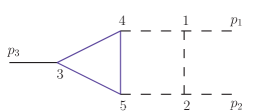
Figure 3: Two-loop vertex graph $P_{126}$, containing a massive triangle loop. Solid lines are massive, dashed lines are massless. The vertices are labeled to match the construction of the integrand from the topology as explained in the text.

The template file templateP126.m in the demos subdirectory contains the following lines:
proplist={{ms[1],{3,4}},{ms[1],{4,5}},{ms[1],{5,3}},{0,{1,2}},{0,{1,4}},{0,{2,5}}};
onshell={ssp[1]$\to$ 0,ssp[2]$\to$ 0,ssp[3]$\to$ sp[1,2]};
where each entry in proplist corresponds to a propagator of the diagram; the first entry is the mass of the propagator, and the second entry contains the labels of the two vertices which the propagator connects. The labels for the vertices are as shown in Fig. 3. Note that if an external momentum $p_{k}$ is flowing into the vertex, the vertex must also have the label $k$. For vertices containing only internal propagators the labeling is arbitrary. The on-shell conditions in the above example state that $p_{1}^{2}=p_{2}^{2}=0,\,p_{3}^{2}=s_{12}=s$. Results for the $\epsilon^{0}$ part of graph $P_{126}$ are shown in Fig. 4.

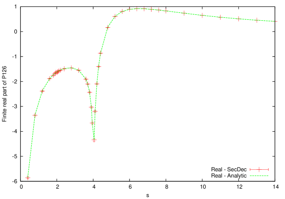
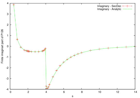
Figure 4: Comparison of analytic and numerical results for the diagram $P_{126}$ using $m^{2}=1$.

To run this example, from the loop directory, issue the command ./launch -d demos -p paramP126.input -t templateP126.m. The timings for the finite part and a relative accuracy of about 1%, using Cuba-3.0 [60], are around 100 secs for a typical point far from the $s=4m^{2}$ threshold on an Intel(R) Core(TM) i7 CPU at 2.67GHz with eight cores. For a point close to threshold ($s/m^{2}=3.9$), the timings are similar.

Producing data files for sets of numerical values

To loop over a set of numerical values for the invariants $s$ and $m^{2}$ once the C++ files are created, issue the command
perl multinumerics.pl -d demos -p multiparamP126.input. This will run the numerical integrations for the values of $s$ and $m^{2}$ specified in the file demos/multiparamP126.input. The files containing the results will be found in demos/2loop/P126, and the files p-2.gpdat, p-1.gpdat and p0.gpdat will contain the data files for each point, corresponding to the coefficients of $\epsilon^{-2},\epsilon^{-1}$ and $\epsilon^{0}$ respectively. These files can be used to plot the results against the analytic results using gnuplot. This will produce the files P126R0.ps, P126I0.ps which will look like Fig. 4.

5.1.2 Non-planar massive two-loop four-point functions

The graph $B_{6}^{NP}$

Figure 5: The non-planar 6-propagator graph $B_{6}^{NP}$.

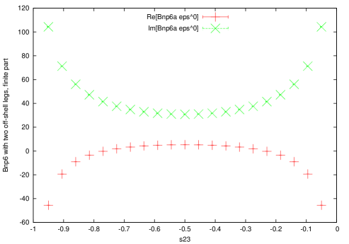
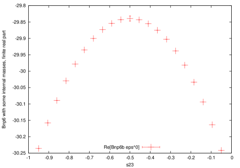
Figure 6: Results for the finite part of the graph $B_{6}^{NP}$ (a) with $p_{1}^{2}$ and $p_{2}^{2}$ off-shell, (b) with $m_{1}=m_{2}=m_{5}=m_{6}=0.25,m_{3}=m_{4}=0.$ The imaginary part of $B_{6}^{NP,b}$ is zero in the range shown above.

Next, we consider the non-planar 6-propagator two-loop four-point diagram shown in Fig. 5. For light-like legs and massless propagators, the analytic result has been calculated in [65], where the graph is called $B_{6}^{NP}$. Here we give results for this topology for the cases where
(a) $p_{1}^{2}$ and $p_{2}^{2}$ are off-shell
(b) $m_{1}=m_{2}=m_{5}=m_{6}\not=0,m_{3}=m_{4}=0.$
It is interesting to note that $B_{6}^{NP,a}$ with $p_{1}^{2}$ and $p_{2}^{2}$ being off-shell contains poles starting from $1/\epsilon^{4}$, while for light-like legs the leading pole is only $1/\epsilon^{2}$, due to cancellations related to the high symmetry of the graph. For $B_{6}^{NP,b}$, i.e. the graph with $m_{1}=m_{2}=m_{5}=m_{6}\not=0$, the leading pole is $1/\epsilon$. Results for the finite parts of $B_{6}^{NP,a}$ and $B_{6}^{NP,b}$ are shown in Figs. 6 and 7.

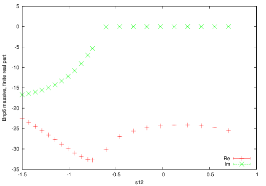
Figure 7: The non-planar 6-propagator graph $B_{6}^{NP,b}$ as a function of $s_{12}$ in a region containing a threshold.

As in [65], an overall prefactor of $\Gamma(1+2\epsilon)\Gamma(1-\epsilon)^{3}/\Gamma(1-3\epsilon)/(1+4\epsilon)$ has been extracted. For Fig. 6 we have used the numerical values $s_{12}=3$ while scanning over $s_{23}$. For all the values given, $s_{13}$ is determined by the physical constraint $s_{12}+s_{13}+s_{23}=p_{1}^{2}+p_{2}^{2}$. For $B_{6}^{NP,a}$ we have set $p_{1}^{2}=p_{2}^{2}=1$, while for $B_{6}^{NP,b}$, $m_{1}=m_{2}=m_{5}=m_{6}=0.25$ has been used. Fig. 7 shows $B_{6}^{NP,b}$ as a function of $s_{12}$ with $s_{23}=-0.4$ and $m_{1}=m_{2}=m_{5}=m_{6}=0.25$. The numerical accuracy is about one permil, therefore the error bars are barely seen in the figures.

The graph $J^{NP}$

In this example we consider a 7-propagator non-planar two-loop box integral where all propagators are massive, using $m_{1}=m_{2}=m_{5}=m_{6}=m$, $m_{3}=m_{4}=m_{7}=M$, $p_{1}^{2}=p_{2}^{2}=p_{3}^{2}=p_{4}^{2}=m^{2}$. The labelling is as shown in Fig. 8.

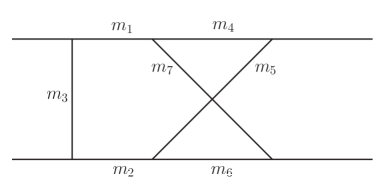
Figure 8: Labeling of the masses for the non-planar graph $J^{NP}$.

Numerical results for this integral have been calculated in [45] using a method based on extrapolation in the $i\delta$ parameter. Our results for $m=50,M=90,s_{23}=-10^{4}$ are shown in Fig. 9 and agreement with ref. [45] has been verified. The timings for the longest subfunction (both real and imaginary part) with a relative accuracy of one permil vary between about 20 seconds for a point far from threshold and about 500 seconds close to threshhold.

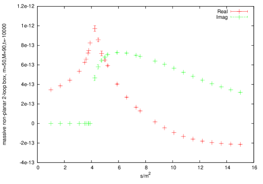
Figure 9: Results for a non-planar 7-propagator graph $J^{NP}$ with all propagators massive using $m=50$, $M=90$ and $t=-10^{4}$.

The graph $ggtt_{1}$

The graph shown in Fig. 10 occurs in the calculation of the two-loop corrections to heavy quark production. Numerical results for the two-loop amplitude in the $q\bar{q}$ initiated channel have been calculated in [51]. Analytic results in the $q\bar{q}$ channel and for some colour structures in the $gg$ channel have been calculated in [66, 67, 68]. Numerical results for the amplitude in the $gg$ channel in the approximation $s\gg m_{t}^{2}$ have been calculated in [69, 70].

For the individual graph shown in Fig. 10, numerical results at Euclidean points have been given in [4]. Here we give numerical results for the non-planar master integral $ggtt_{1}$ in the non-Euclidean region. For the results shown in Fig. 11, we used $s_{23}=-0.4,p_{3}^{2}=p_{4}^{2}=0.25,m_{1}^{2}=m_{2}^{2}=0.25,s_{13}=-s_{12}-s_{23}+p_{3}^{2}+p_{4}^{2}$. The analytical result for this master integral is not known yet.

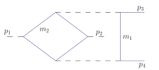
Figure 10: Non-planar graph ocurring in the calculation of $gg\to t\bar{t}$ at NNLO. Blue (solid) lines denote massive particles.

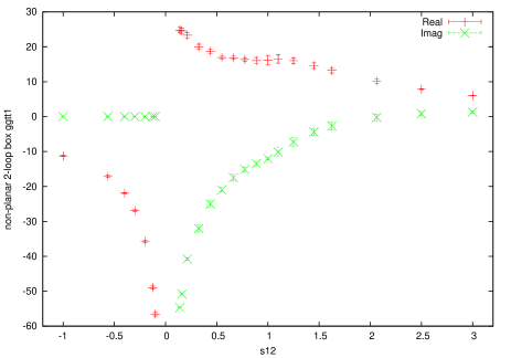
Figure 11: Results for the non-planar graph $ggtt_{1}$.

5.2 Defining implicit functions

This example demonstrates the ability to leave certain functions implicit until numerical integration. Suppose we want to integrate

$$f(\vec{x})=(x_{1}+x_{2})^{-2-2\epsilon}x_{3}^{-1-4\epsilon}dum_{1}(x_{1},x_{2},x_{3},x_{4})^{1+\epsilon}dum_{2}(x_{2},x_{4})^{2-6\epsilon}cut(x_{3})$$

with

$$dum_{1}(x_{1},x_{2},x_{3},x_{4}) = 2+x_{1}^{2}+x_{2}^{3}+x_{3}^{4}+x_{4}^{5}+4x_{1}x_{2}x_{3}x_{4}-x_{1}^{2}x_{2}^{3}x_{3}^{4}x_{4}^{5}$$

$$dum_{2}(x_{2},x_{4}) = x_{2}^{2}+x_{4}^{2}+\beta^{2}+4x_{2}x_{4}-\sqrt{x_{2}x_{4}\beta}+3x_{2}^{2}x_{4}^{2}\;,$$

where $\beta$ is a symbol defined in the parameter file. $dum_{1}$ and $dum_{2}$ should always be functions which cannot increase the singular behaviour of the integrand, and so quantitative knowledge of their exact form is not required to guide the decomposition. Thus they can be left implicit, and only introduced at the numerical integration stage. The function $cut(x)$ is already defined by default as $cut(x)\equiv\Theta(x-cutval)$, where the value of $cutval$ is given in the parameter file. The command ../launch -p paramdummy.input -t templatedummy.m from the folder general/demos runs this example. The fortran files containing the explicit form of the functions $dum_{1}$, $dum_{2}$, $cut$ are found in demos/testdummy. Another simple example for a dummy function would be a jet function as used in the JADE algorithm in $e^{+}e^{-}$ annihilation, as described e.g. in [71]. Input files for such an example are params23s35JADE.input, templates23s35JADE.m in the general/demos directory.

6 Conclusions

We have presented the program SecDec 2.0, which can be used to factorise dimensionally regulated singularities and numerically calculate multi-loop integrals in an automated way. As a new feature of the program, it now can deal with fully physical kinematics, i.e. is not restricted to the Euclidean region anymore. A new construction of the integrand, based entirely on topological rules, is also included. The new features are demonstrated by several examples, among them a massive two-loop four-point function which is not yet known analytically. In addition, the program can produce numerical results for more general parameter integrals, as they occur for example in phase space integrals for multi-particle production with several unresolved massless particles. The program also offers the possibility to include symbolic functions which can be used for instance to define measurement functions like jet algorithms in a flexible way. The program setup is such that the evaluation of several functions in parallel can lead to a major speed-up. To calculate full two-loop amplitudes involving several mass scales, the timings still leave room for improvement, but considering the fact that the method is very suitable for intense parallelisation, we are convinced that the program will be a very useful tool for a multitude of applications to higher order corrections in quantum field theories.

Appendix A User manual

We list here all possible input parameters for the parameter file *.input and the Mathematica input file *.m. These two files serve to define the integrand and the parameters for the numerical integration. We describe here the example of loop diagrams; the input files in the subdirectory general to compute more general parametric functions is very similar.

A.1 Program input parameters

This input file should be called *.input. The following parameters can be specified

subdir

subdir specifies the name of the subdirectory to which the graph should be written to. If not yet existent, it will be created. The specified subdir contains the directory specified in outputdir.

outputdir

The name for the desired output directory can be given here. If outputdir is not specified, the default directory for the output will have the graph name (see below) appended to the directory subdir, otherwise specify the full path for the Mathematica output files here.
The output directory will contain all the files produced during the decomposition, subtraction, expansion and numerical integration, and the results. The output of the decomposition into sectors is found in the outputdir directly. The functions from subtraction and expansion and the respective files for numerical integration are found in subdirectories. The latter are named with the pole structure and contain subdirectories named with the respective Laurent coefficient.

graph

The name of the diagram or parametric function to be computed is specified here. The graph name can contain underscores and numbers, but should not contain commas.

propagators

The number of propagators the diagram has is specified here (mandatory).

legs

The number of external legs the diagram has is specified here (mandatory).

loops

The number of loops the diagram has is specified here (mandatory).

cutconstruct

If the graph to be computed corresponds to a scalar integral, the integrand (F and U) can be constructed via topological cuts. In this case set cutconstruct=1, the default is =0. If cutconstruct is switched on, the input for the graph structure (*.m file) is just a list of labels connecting vertices, as explained in Section 3.4 and A.2.

epsord

The order to which the Laurent series in $\epsilon$ should be expanded, starting from $\epsilon^{-maxpole}$, can be specified here. The default is epsord=0 where the Laurent series is cut after finite part $\epsilon^{0}$. If epsord is set to a negative value, only the pole coefficients up to this order will be computed.

prefactorflag

Possible values for the prefactorflag are 0 (default), 1 and 2.

• 0: The default prefactor $(-1)^{N}\,\Gamma[N-Nloops*Dim/2]$ is factored out of the numerical result.

• 1: The default prefactor $(-1)^{N}\,\Gamma[N-Nloops*Dim/2]$ is included in the numerical result.

• 2: Give the desired prefactor to be factored out in prefactor.

prefactor

If option 2 has been chosen in the prefactorflag, write down the desired prefactor in Mathematica syntax here. In combination with options 0 or 1 in the prefactorflag this entry will be ignored Use Nn, Nloops and Dim to denote the number of propagators, loops and dimension (4-2eps by default).

IBPflag

Set IBPflag=0 if integration by parts should not be used, =1 if it should be used. IBPflag=2 is designed to use IBP when it is more efficient to do so, and not otherwise. Using the integrations by parts method takes more time in the subtraction and expansion step and generally results in more functions for numerical integration. However, it can be useful if (spurious) poles of type $x^{-2-b\epsilon}$ are found in the decomposition, as it reduces the power of $x$ in the denominator.

compiler

Set a Fortran compiler (tested with gfortran, ifort, g77) if language=Fortran. Left blank, the default is gfortran.

exeflag

The exeflag is set to decide at which stage the program terminates:

• 0: The iterated sector decomposition is done and the scripts to do the subtraction, the expansion in epsilon, the creation of the Fortran/C++ files and to launch the numerical integration are created (scripts batch* in the subdirectory graph) but not run. This can be useful if a cluster is available to run each pole structure on a different node.

• 1: In addition to the steps done in 0, the subtraction and epsilon expansion is performed and the resulting functions are written to Fortran/C++ files.

• 2: In addition to the steps done in 1, all the files needed for the numerical integration are created.

• 3: In addition to the steps done in 2, the compilation of the Fortran/C++ files is launched to make the executables.

• 4: In addition to the steps done in 3, the executables are run, either by batch submission or locally.

clusterflag

The clusterflag determines how jobs are submitted. Setting clusterflag=0 (default) the jobs will run on a single machine, setting it =1 the jobs will run on a cluster (a batch system to submit jobs).

batchsystem

If a cluster is used (clusterflag=1), this flag should be set to 0 to use the setup for the PBS (Portable batch system). If the flag is set to 1 a user-defined setup is activated. Currently this is the submission via condor, but the user can adapt this to his needs by editing perlsrc/makejob.pm.

maxjobs

When using a cluster, specify the maximum number of jobs allowed in the queue here.

maxcput

Specify here the estimated maximal CPU time (in hours). This option is used to send a job to a particular queue on a batch system, otherwise it is not important.

pointname

The name of the point to calculate is specified here. It should be either blank or a string and is useful to label the result files in case of different runs for different numerical values of the Mandelstam variables, masses etc.

sij

The values for Mandelstam invariants $s_{ij}=(p_{i}+p_{j})^{2}$ in numbers are specified here (mandatory). The $s_{ij}$ should be $\leq 0$ in the Euclidean region.

pi2

The off-shell legs $p_{1}^{2}$, $p_{2}^{2}$,… are specified here (mandatory). $p_{i}^{2}$ should be $\leq 0$ in the Euclidean region.

ms2

Specify the masses of propagators $m_{1}^{2}$, $m_{2}^{2}$,… here using the notation ms[i] for $m_{i}^{2}$ (mandatory). The masses should not be complex numbers.

integrator

The program for numerical integration can be chosen here. BASES (integrator=0) can only be used in the Fortran version. Vegas (integrator=1), Suave (integrator=2), Divonne (integrator=3, default) and Cuhre (integrator=4) are part of the Cuba library and can be used in both the Fortran and the C++ version. In practice, Divonne usually gives the fastest results when using the C++ version. In the following we therefore concentrate on the adjustment of the parameters needed for numerical integration using Divonne. For more details about the Cuba parameters we refer to [59].

cubapath

The path to the Cuba library can be specified here. The default directory is [your path to SecDec]/Cuba-3.0. Cuba-3.0 is the newest version of the Cuba library and uses parallel processing during the numerical evaluation of the integral. The older version (Cuba-2.1) is still supported and can be used.

maxeval

Separated by commas and starting with the lowest order coefficient in $\epsilon$, specify the maximal number of evaluations to be used by the numerical integrator for each order in $\epsilon$. If maxeval is not equal to mineval, the maximal number of evaluations does not have to be reached.

mineval

Separated by commas and starting with the lowest order coefficient in $\epsilon$, specify the number of evaluations which should at least be done before the numerical integrator returns a result. The default is 0.

epsrel

Separated by commas and starting with the lowest order coefficient in $\epsilon$, specify the desired relative accuracy for the numerical evaluation.

epsabs

Separated by commas and starting with the lowest order coefficient in $\epsilon$, specify the desired absolute accuracy for the numerical evaluation. This becomes useful in the cases where the integrated result is close to zero.

cubaflags

Set the cuba verbosity flags. The default is 2 which means, the Cuba input parameters and other useful information, e.g. about numerical convergence, are echoed during numerical integration.

key1

Separated by commas and starting with the lowest order coefficient in $\epsilon$, specify key1 which determines the sampling to be used for the partitioning phase in Divonne. With a positive key1, a Korobov quasi-random sample of key1 points is used. A key1 of about 1000 (default) usually is a good choice.

key2

Separated by commas and starting with the lowest order coefficient in $\epsilon$, specify key2 which determines the sampling to be used for the final integration phase in Divonne. With a positive key2, a Korobov quasi-random sample is used. The default is key2=1 which means, the number of points needed to reach the prescribed accuracy is estimated by Divonne.

key3

Separated by commas and starting with the lowest order coefficient in $\epsilon$, specify the key3 to be used for the refinement phase in Divonne. Setting key3=1 (default), each subregion is split once more.

maxpass

Separated by commas and starting with the lowest order coefficient in $\epsilon$, specify how good the convergence has to be during the partitioning phase until the program passes on to the main integration phase. A maxpass of 3 (default) is usually sufficient to get a quick and good result.

border

Separated by commas and starting with the lowest order coefficient in $\epsilon$, specify the border for the numerical integration. The points in the interval $[0,border]$ and $[1-border,1]$ are not included in the integration but are extrapolated from points further from the endpoints. This can be useful if the integrand is known to be peaked at endpoints of the integration variables.

maxchisq

Separated by commas and starting with the lowest order coefficient in $\epsilon$, specify the maximally allowed $\chi^{2}$ at the end of the numerical integration.

mindeviation

Separated by commas and starting with the lowest order coefficient in $\epsilon$, specify the deviation two sample averages in one region can show without being treated any further.

These parameters are advanced options

primarysectors

Specify a list of primary sectors to be treated here. If left blank, primarysectors defaults to all, i.e. 1 to the number of propagators, will be taken. This option is useful if a diagram has symmetries such that some primary sectors yield the same result.

multiplicities

Specify the multiplicities of the primary sectors listed above. List the multiplicities in same order as the corresponding sectors above. If left blank, default multiplicities (=one) are set automatically.

infinitesectors

A list of primary sectors to be redone differently because they lead to infinite recursion can be specified here. infinitesectors must be left empty for the default strategy to be applied.

togetherflag

This flag defines whether to integrate subsets of functions for each pole order separately togetherflag=0(default) or to sum all functions for a certain pole order and then integrate togetherflag=1. The latter will allow cancellations between different functions and thus give a more realistic error, but should not be used for complicated diagrams where the individual functions are large already.

editor

Choose here which editor should be used to display the result. If editor=none is set, the full result will not be displayed in an editor window at the end of the calculation.

grouping

If the togetherflag is set to 0, it could still be useful to first sum a few functions before integration. The number of bytes you set with grouping=#bytes decides how many functions f*.f or f*.cc are first summed and only then integrated with the numerical integrator. If you set grouping=0 all functions f*.f resp. f*.cc are integrated separately. In practice, a grouping=0 has proven to lead to faster convergence and more accurate results. However, if you consider integrals which show large cancellations within the different functions f*.cc, it might be useful to use a grouping$\neq 0$. The log files *results*.log in the results directory contain the results from the individual integration, where the user can see if there are large cancellations between the individual functions.

language

For one-scale diagrams or diagrams with purely Euclidean kinematics language=fortran or language=Cpp (default) can be chosen, where the Cpp stands for C++.
In all other cases, especially when using contourdef=True, language=Cpp is used, as the deformation of the contour which is needed for these problems is only implemented in C++.

rescale

If all invariants are very small or very large it is useful to rescale them to reach faster convergence during numerical integration. The rescaling (scaling out the largest invariant in the numerical integration part) can be switched on with rescale=1 and switched off when set to 0. If switched on, it is not possible to set explicit values of any non-zero invariants in the Mathematica input file template*.m.

contourdef

For multi-scale problems resp. diagrams with non-Euclidean kinematics, set contourdef=True (default is False). In this case, a deformation of the integration contour in the form of Eq. (2.2) is done. In addition to the functions f*.cc to be integrated, auxiliary files (g*.cc) are written which serve to optimize the deformation for each integrand function.

lambda

Here, you can set the initial lambda $\lambda$ for the deformation of Eq. (2.2). Without any knowledge about the characteristics of the integrand, lambda=1.0 should be a good choice. If the diagram contains mostly massless propagators and light-like legs, it can be useful to choose the initial $\lambda$ larger (e.g.lambda=5.0), in order to compensate for cases where the remainders of the IR subtraction lead to large cancellations for $x_{i}\to 0$. For diagrams with mostly massive propagators the initial lambda can be chosen smaller (e.g.lambda=0.1).

smalldefs

If the integrand is expected to be oscillatory and hence sensitive to small changes in the deformation parameter $\lambda$, smalldefs should be set to 1 (default is 0). If switched on, the argument of each subsector function ${\cal F}$ is minimized.

largedefs

If the integrand is expected to have (integrable) endpoint singularities at $x_{j}=0$ or 1, the deformation should be large in order to move the contour away from the problematic region. If largedefs=1, the program tries to enlarge the deformation at the endpoints. The default is largedefs=0.

A.2 Input for the definition of the integrand

This Mathematica input file should be called *.m. The following parameters can be specified

momlist

If cutconstruct=0 is set in the input file, specify the names of the loop momenta here.

proplist

Specify the diagram topology here (mandatory). The syntax for cutconstruct=1 is described in Section 3.4. If cutconstruct=0 has been chosen, the propagators have to be given explicitly. An example propagator list could be proplist={k^2-ms[1],(k+p1)^2-ms[1]} with the loop momentum $k$, the propagator mass $m_{1}^{2}$ and external momentum $p_{1}$.

numerator

If present, specify the numerator of the integrand here. If not given, a numerator={1} is assumed. Please note that the option cutconstruct=1 is not available in combination with numerator functions.

powerlist

As an option, the propagator powers (e.g. if different from one) can be set here.

onshell

Specify invariant replacements here. The kinematic invariants can be assigned values (e.g. ssp[1]$\to$0) or relations between the invariants can be set (e.g. ssp[1]$\to$sp[1,3]). This option can not be used in combination with rescale=1.

Dim

Set the space-time dimension. The default is Dim=4-2 eps and the symbol for the regulator $\epsilon$ must remain the same.

References

- [1] T. Binoth and G. Heinrich. An automatized algorithm to compute infrared divergent multi-loop integrals. Nucl. Phys., B585:741–759, 2000.
- [2] M. Roth and Ansgar Denner. High-energy approximation of one-loop Feynman integrals. Nucl. Phys., B479:495–514, 1996.
- [3] Klaus Hepp. Proof of the Bogolyubov-Parasiuk theorem on renormalization. Commun. Math. Phys., 2:301–326, 1966.
- [4] Jonathon Carter and Gudrun Heinrich. SecDec: A general program for sector decomposition. Comput.Phys.Commun., 182:1566–1581, 2011.
- [5] Christian Bogner and Stefan Weinzierl. Resolution of singularities for multi-loop integrals. Comput. Phys. Commun., 178:596–610, 2008.
- [6] A.V. Smirnov and M.N. Tentyukov. Feynman Integral Evaluation by a Sector decomposiTion Approach (FIESTA). Comput.Phys.Commun., 180:735–746, 2009.
- [7] A.V. Smirnov, V.A. Smirnov, and M. Tentyukov. FIESTA 2: Parallelizeable multiloop numerical calculations. Comput.Phys.Commun., 182:790–803, 2011.
- [8] Janusz Gluza, Krzysztof Kajda, Tord Riemann, and Valery Yundin. Numerical Evaluation of Tensor Feynman Integrals in Euclidean Kinematics. Eur.Phys.J., C71:1516, 2011.
- [9] Takahiro Ueda and Junpei Fujimoto. New implementation of the sector decomposition on FORM. PoS, ACAT08:120, 2008.
- [10] Gudrun Heinrich. Sector Decomposition. Int. J. Mod. Phys., A23:1457–1486, 2008.
- [11] Charalampos Anastasiou, Franz Herzog, and Achilleas Lazopoulos. On the factorization of overlapping singularities at NNLO. JHEP, 1103:038, 2011. 36 pages.
- [12] Volker Pilipp. Semi-numerical power expansion of Feynman integrals. JHEP, 0809:135, 2008.
- [13] M. Czakon, J. Gluza, and T. Riemann. Master integrals for massive two-loop Bhabha scattering in QED. Phys. Rev., D71:073009, 2005.
- [14] Ansgar Denner and S. Pozzorini. An algorithm for the high-energy expansion of multi-loop diagrams to next-to-leading logarithmic accuracy. Nucl. Phys., B717:48–85, 2005.
- [15] Ansgar Denner, Bernd Jantzen, and Stefano Pozzorini. Two-loop electroweak next-to-leading logarithms for processes involving heavy quarks. JHEP, 0811:062, 2008.
- [16] M. Czakon. A novel subtraction scheme for double-real radiation at NNLO. Phys.Lett., B693:259–268, 2010. 14 pages, 3 figures, matches published version, includes new name for the scheme, extended discussion of massless final states, and some new references.
- [17] M. Czakon. Double-real radiation in hadronic top quark pair production as a proof of a certain concept. Nucl.Phys., B849:250–295, 2011. 44 pages, 10 figures.
- [18] Radja Boughezal, Kirill Melnikov, and Frank Petriello. A subtraction scheme for NNLO computations. Phys.Rev., D85:034025, 2012. 13 pages.
- [19] Paolo Bolzoni, Gabor Somogyi, and Zoltan Trocsanyi. A subtraction scheme for computing QCD jet cross sections at NNLO: integrating the iterated singly-unresolved subtraction terms. JHEP, 1101:059, 2011. 83 pages, one reference added, typos corrected, agrees with published version.
- [20] Gudrun Heinrich. A numerical method for NNLO calculations. Nucl. Phys. Proc. Suppl., 116:368–372, 2003.
- [21] Charalampos Anastasiou, Kirill Melnikov, and Frank Petriello. A new method for real radiation at NNLO. Phys. Rev., D69:076010, 2004.
- [22] A. Gehrmann-De Ridder, T. Gehrmann, and G. Heinrich. Four-particle phase space integrals in massless QCD. Nucl. Phys., B682:265–288, 2004.
- [23] T. Binoth and G. Heinrich. Numerical evaluation of phase space integrals by sector decomposition. Nucl. Phys., B693:134–148, 2004.
- [24] Charalampos Anastasiou, Kirill Melnikov, and Frank Petriello. Real radiation at NNLO: jets through O. Phys. Rev. Lett., 93:032002, 2004.
- [25] Giampiero Passarino and Sandro Uccirati. Algebraic numerical evaluation of Feynman diagrams: Two loop selfenergies. Nucl.Phys., B629:97–187, 2002.
- [26] Andrea Ferroglia, Massimo Passera, Giampiero Passarino, and Sandro Uccirati. All purpose numerical evaluation of one loop multileg Feynman diagrams. Nucl.Phys., B650:162–228, 2003.
- [27] Andrea Ferroglia, Massimo Passera, Giampiero Passarino, and Sandro Uccirati. Two loop vertices in quantum field theory: Infrared convergent scalar configurations. Nucl.Phys., B680:199–270, 2004.
- [28] Stefano Actis, Andrea Ferroglia, Giampiero Passarino, Massimo Passera, and Sandro Uccirati. Two-loop tensor integrals in quantum field theory. Nucl.Phys., B703:3–126, 2004.
- [29] Giampiero Passarino and Sandro Uccirati. Two-loop vertices in quantum field theory: Infrared and collinear divergent configurations. Nucl.Phys., B747:113–189, 2006. 62 pages, 15 figures, 16 tables.
- [30] Stefano Actis, Giampiero Passarino, Christian Sturm, and Sandro Uccirati. NNLO Computational Techniques: The Cases H to gamma gamma and H to g g. Nucl.Phys., B811:182–273, 2009. LaTeX, 70 pages, 8 eps figures.
- [31] Davison E. Soper. Techniques for QCD calculations by numerical integration. Phys. Rev., D62:014009, 2000.
- [32] T. Binoth, G. Heinrich, and N. Kauer. A numerical evaluation of the scalar hexagon integral in the physical region. Nucl. Phys., B654:277–300, 2003.
- [33] Zoltan Nagy and Davison E. Soper. Numerical integration of one-loop Feynman diagrams for N-photon amplitudes. Phys. Rev., D74:093006, 2006.
- [34] T. Binoth, J. Ph. Guillet, G. Heinrich, E. Pilon, and C. Schubert. An algebraic / numerical formalism for one-loop multi-leg amplitudes. JHEP, 10:015, 2005.
- [35] Wei Gong, Zoltan Nagy, and Davison E. Soper. Direct numerical integration of one-loop Feynman diagrams for N-photon amplitudes. Phys. Rev., D79:033005, 2009.
- [36] Achilleas Lazopoulos, Kirill Melnikov, and Frank Petriello. QCD corrections to tri-boson production. Phys. Rev., D76:014001, 2007.
- [37] Achilleas Lazopoulos, Thomas McElmurry, Kirill Melnikov, and Frank Petriello. Next-to-leading order QCD corrections to production at the LHC. Phys.Lett., B666:62–65, 2008.
- [38] Sebastian Becker, Christian Reuschle, and Stefan Weinzierl. Numerical NLO QCD calculations. JHEP, 1012:013, 2010.
- [39] Sebastian Becker, Daniel Goetz, Christian Reuschle, Christopher Schwan, and Stefan Weinzierl. NLO results for five, six and seven jets in electron-positron annihilation. Phys.Rev.Lett., 108:032005, 2012. 5 pages.
- [40] Y. Kurihara and T. Kaneko. Numerical contour integration for loop integrals. Comput.Phys.Commun., 174:530–539, 2006.
- [41] Charalampos Anastasiou, Stefan Beerli, and Alejandro Daleo. Evaluating multi-loop Feynman diagrams with infrared and threshold singularities numerically. JHEP, 05:071, 2007.
- [42] Charalampos Anastasiou, Stefan Beerli, and Alejandro Daleo. The two-loop QCD amplitude gg -¿ h,H in the Minimal Supersymmetric Standard Model. Phys. Rev. Lett., 100:241806, 2008.
- [43] Stefan Beerli. A New method for evaluating two-loop Feynman integrals and its application to Higgs production. 2008. Ph.D. Thesis (Advisor: Zoltan Kunszt).
- [44] E. de Doncker, Y. Shimizu, J. Fujimoto, and F. Yuasa. Computation of loop integrals using extrapolation. Comput.Phys.Commun., 159:145–156, 2004.
- [45] F. Yuasa, E. de Doncker, N. Hamaguchi, T. Ishikawa, K. Kato, et al. Numerical Computation of Two-loop Box Diagrams with Masses. 2011.
- [46] S. Bauberger, Frits A. Berends, M. Bohm, and M. Buza. Analytical and numerical methods for massive two loop selfenergy diagrams. Nucl.Phys., B434:383–407, 1995.
- [47] Junpei Fujimoto, Yoshimitsu Shimizu, Kiyoshi Kato, and Toshiaki Kaneko. Numerical approach to two loop three point functions with masses. Int.J.Mod.Phys., C6:525–530, 1995.
- [48] Michele Caffo, H. Czyz, and E. Remiddi. Numerical evaluation of the general massive 2 loop sunrise selfmass master integrals from differential equations. Nucl.Phys., B634:309–325, 2002.
- [49] S. Pozzorini and E. Remiddi. Precise numerical evaluation of the two loop sunrise graph master integrals in the equal mass case. Comput.Phys.Commun., 175:381–387, 2006.
- [50] M. Czakon. Automatized analytic continuation of Mellin-Barnes integrals. Comput.Phys.Commun., 175:559–571, 2006.
- [51] M. Czakon. Tops from Light Quarks: Full Mass Dependence at Two-Loops in QCD. Phys.Lett., B664:307–314, 2008.
- [52] Ayres Freitas and Yi-Cheng Huang. On the Numerical Evaluation of Loop Integrals With Mellin-Barnes Representations. JHEP, 1004:074, 2010.
- [53] O. V. Tarasov. Connection between Feynman integrals having different values of the space-time dimension. Phys. Rev., D54:6479–6490, 1996.
- [54] Vladimir A. Smirnov. Feynman integral calculus. Springer, 2006.
- [55] L. D. Landau. On analytic properties of vertex parts in quantum field theory. Nucl. Phys., 13:181–192, 1959.
- [56] R. J. Eden, P. V. Landshoff, David I. Olive, and J. C. Polkinghorne. The Analytic S-Matrix. Cambridge University Press, 1966.
- [57] N. Nakanishi. Graph Theory and Feynman Integrals. Gordon and Breach, New York, 1971.
- [58] Mathematica, Copyright by Wolfram Research.
- [59] T. Hahn. CUBA: A library for multidimensional numerical integration. Comput. Phys. Commun., 168:78–95, 2005.
- [60] S. Agrawal, T. Hahn, and E. Mirabella. FormCalc 7. 2011.
- [61] Setsuya Kawabata. A New version of the multidimensional integration and event generation package BASES/SPRING. Comp. Phys. Commun., 88:309–326, 1995.
- [62] Frans Slothouber and et al. ROBODoc 4.99.40. http://www.xs4all.nl/ rfsber/Robo/robodoc.html.
- [63] R. Bonciani, P. Mastrolia, and E. Remiddi. Master integrals for the two loop QCD virtual corrections to the forward backward asymmetry. Nucl.Phys., B690:138–176, 2004.
- [64] Andrei I. Davydychev and M.Yu. Kalmykov. Massive Feynman diagrams and inverse binomial sums. Nucl.Phys., B699:3–64, 2004.
- [65] J.B. Tausk. Nonplanar massless two loop Feynman diagrams with four on-shell legs. Phys.Lett., B469:225–234, 1999.
- [66] R. Bonciani, A. Ferroglia, T. Gehrmann, D. Maitre, and C. Studerus. Two-Loop Fermionic Corrections to Heavy-Quark Pair Production: The Quark-Antiquark Channel. JHEP, 0807:129, 2008.
- [67] R. Bonciani, A. Ferroglia, T. Gehrmann, and C. Studerus. Two-Loop Planar Corrections to Heavy-Quark Pair Production in the Quark-Antiquark Channel. JHEP, 0908:067, 2009.
- [68] R. Bonciani, A. Ferroglia, T. Gehrmann, A. Manteuffel, and C. Studerus. Two-Loop Leading Color Corrections to Heavy-Quark Pair Production in the Gluon Fusion Channel. JHEP, 1101:102, 2011.
- [69] M. Czakon, A. Mitov, and S. Moch. Heavy-quark production in massless quark scattering at two loops in QCD. Phys.Lett., B651:147–159, 2007.
- [70] M. Czakon, A. Mitov, and S. Moch. Heavy-quark production in gluon fusion at two loops in QCD. Nucl.Phys., B798:210–250, 2008.
- [71] S. Bethke et al. Experimental Investigation of the Energy Dependence of the Strong Coupling Strength. Phys.Lett., B213:235, 1988.