Analysis of a Natural Gradient Algorithm on Monotonic Convex-Quadratic-Composite Functions

Youhei Akimoto

Project TAO INRIA Saclay, LRI Université Paris-Sud, 91405 Orsay Cedex, France Youhei.Akimoto@lri.fr
(2012)
Abstract

In this paper we investigate the convergence properties of a variant of the Covariance Matrix Adaptation Evolution Strategy (CMA-ES). Our study is based on the recent theoretical foundation that the pure rank-μ𝜇\mu update CMA-ES performs the natural gradient descent on the parameter space of Gaussian distributions. We derive a novel variant of the natural gradient method where the parameters of the Gaussian distribution are updated along the natural gradient to improve a newly defined function on the parameter space. We study this algorithm on composites of a monotone function with a convex quadratic function. We prove that our algorithm adapts the covariance matrix so that it becomes proportional to the inverse of the Hessian of the original objective function. We also show the speed of covariance matrix adaptation and the speed of convergence of the parameters. We introduce a stochastic algorithm that approximates the natural gradient with finite samples and present some simulated results to evaluate how precisely the stochastic algorithm approximates the deterministic, ideal one under finite samples and to see how similarly our algorithm and the CMA-ES perform.

category:
G.1.6 Numerical Analysis Optimization
keywords:
Global optimization, Gradient methods, Unconstrained optimization
category:
F.2.1 Analysis of Algorithms and Problem Complexity Numerical Algorithms and Problems
keywords:
Covariance Matrix Adaptation, Natural Gradient, Hessian Matrix, Information Geometric Optimization, Theory
conference: GECCO’12, July 7-11, 2012, Philadelphia, Pennsylvania, USA.terms: Algorithms, Theory

Errata

Errata in the original GECCO’2012 paper (which have been revised in this version)

  • Eq. (21) in Theorem 4
    In the original paper:

    Cond(CtA)1+(12γC,min1γC,min)t(Cond(C0A1).\operatorname{Cond}(C^{t}A)\leqslant 1+\left(\frac{1-2\gamma_{C,\mathrm{min}}}{1-\gamma_{C,\mathrm{min}}}\right)^{t}(\operatorname{Cond}(C^{0}A-1).

    In this version:

    Cond(CtA)1+(1γC,min)t(Cond(C0A)1).Condsuperscript𝐶𝑡𝐴1superscript1subscript𝛾𝐶min𝑡Condsuperscript𝐶0𝐴1\operatorname{Cond}(C^{t}A)\leqslant 1+(1-\gamma_{C,\mathrm{min}})^{t}(\operatorname{Cond}(C^{0}A)-1).
  • The paragraph after (24)
    In the original paper:
    Since

    1ηCt(λ1t+λdt)(1ηCtλdt)=1ηCtλ1t(1+λdt/λ1t)1ηCtλ1t(λdt/λ1t)12ηCtλ1t1ηCtλ1t,1superscriptsubscript𝜂𝐶𝑡superscriptsubscript𝜆1𝑡superscriptsubscript𝜆𝑑𝑡1superscriptsubscript𝜂𝐶𝑡superscriptsubscript𝜆𝑑𝑡1superscriptsubscript𝜂𝐶𝑡superscriptsubscript𝜆1𝑡1superscriptsubscript𝜆𝑑𝑡superscriptsubscript𝜆1𝑡1superscriptsubscript𝜂𝐶𝑡superscriptsubscript𝜆1𝑡superscriptsubscript𝜆𝑑𝑡superscriptsubscript𝜆1𝑡12superscriptsubscript𝜂𝐶𝑡superscriptsubscript𝜆1𝑡1superscriptsubscript𝜂𝐶𝑡superscriptsubscript𝜆1𝑡\frac{1-\eta_{C}^{t}(\lambda_{1}^{t}+\lambda_{d}^{t})}{(1-\eta_{C}^{t}\lambda_{d}^{t})}=\frac{1-\eta_{C}^{t}\lambda_{1}^{t}(1+\lambda_{d}^{t}/\lambda_{1}^{t})}{1-\eta_{C}^{t}\lambda_{1}^{t}(\lambda_{d}^{t}/\lambda_{1}^{t})}\leqslant\frac{1-2\eta_{C}^{t}\lambda_{1}^{t}}{1-\eta_{C}^{t}\lambda_{1}^{t}},

    we have

    Cond(Ct+1A)1Cond(CtA)112ηCtλ1t1ηCtλ1t.Condsuperscript𝐶𝑡1𝐴1Condsuperscript𝐶𝑡𝐴112superscriptsubscript𝜂𝐶𝑡superscriptsubscript𝜆1𝑡1superscriptsubscript𝜂𝐶𝑡superscriptsubscript𝜆1𝑡\frac{\operatorname{Cond}(C^{t+1}A)-1}{\operatorname{Cond}(C^{t}A)-1}\leqslant\frac{1-2\eta_{C}^{t}\lambda_{1}^{t}}{1-\eta_{C}^{t}\lambda_{1}^{t}}.

    Moreover, since the right-hand side of the above inequality is maximized when ηCtλ1tsuperscriptsubscript𝜂𝐶𝑡superscriptsubscript𝜆1𝑡\eta_{C}^{t}\lambda_{1}^{t} is minimized and ηCtλ1tsuperscriptsubscript𝜂𝐶𝑡superscriptsubscript𝜆1𝑡\eta_{C}^{t}\lambda_{1}^{t} is bounded from below by γC,minsubscript𝛾𝐶min\gamma_{C,\mathrm{min}} because of (23), we have

    Cond(Ct+1A)1Cond(CtA)112γC,min1γC,min.Condsuperscript𝐶𝑡1𝐴1Condsuperscript𝐶𝑡𝐴112subscript𝛾𝐶min1subscript𝛾𝐶min\frac{\operatorname{Cond}(C^{t+1}A)-1}{\operatorname{Cond}(C^{t}A)-1}\leqslant\frac{1-2\gamma_{C,\mathrm{min}}}{1-\gamma_{C,\mathrm{min}}}.

    This implies limtCond(CtA)=1subscript𝑡Condsuperscript𝐶𝑡𝐴1\lim_{t\to\infty}\operatorname{Cond}(C^{t}A)=1. The rate of convergence (20) and the upper bound (21) are immediate consequences of the above inequality.

    In this version:
    Since

    1ηCt(λ1t+λdt)(1ηCtλdt)=1ηCtλ1t1ηCtλ1tCond1(CtA)1ηCtλ1t1superscriptsubscript𝜂𝐶𝑡superscriptsubscript𝜆1𝑡superscriptsubscript𝜆𝑑𝑡1superscriptsubscript𝜂𝐶𝑡superscriptsubscript𝜆𝑑𝑡1superscriptsubscript𝜂𝐶𝑡superscriptsubscript𝜆1𝑡1superscriptsubscript𝜂𝐶𝑡superscriptsubscript𝜆1𝑡superscriptCond1superscript𝐶𝑡𝐴1superscriptsubscript𝜂𝐶𝑡superscriptsubscript𝜆1𝑡\frac{1-\eta_{C}^{t}(\lambda_{1}^{t}+\lambda_{d}^{t})}{(1-\eta_{C}^{t}\lambda_{d}^{t})}=1-\frac{\eta_{C}^{t}\lambda_{1}^{t}}{1-\eta_{C}^{t}\lambda_{1}^{t}\operatorname{Cond}^{-1}(C^{t}A)}\leqslant 1-\eta_{C}^{t}\lambda_{1}^{t}

    and the right-most side of the above inequality is bounded by 1γC,min1subscript𝛾𝐶min1-\gamma_{C,\mathrm{min}} because of (23), we have

    Cond(Ct+1A)1Cond(CtA)11γC,min.Condsuperscript𝐶𝑡1𝐴1Condsuperscript𝐶𝑡𝐴11subscript𝛾𝐶min\frac{\operatorname{Cond}(C^{t+1}A)-1}{\operatorname{Cond}(C^{t}A)-1}\leqslant 1-\gamma_{C,\mathrm{min}}.

    This implies limtCond(CtA)=1subscript𝑡Condsuperscript𝐶𝑡𝐴1\lim_{t\to\infty}\operatorname{Cond}(C^{t}A)=1 and (21). Moreover, since limtCond(CtA)=limtλ1t/λdt=1subscript𝑡Condsuperscript𝐶𝑡𝐴subscript𝑡superscriptsubscript𝜆1𝑡superscriptsubscript𝜆𝑑𝑡1\lim_{t\to\infty}\operatorname{Cond}(C^{t}A)=\lim_{t\to\infty}\lambda_{1}^{t}/\lambda_{d}^{t}=1, we have from (24) that

    lim suptCond(Ct+1A)1Cond(CtA)1subscriptlimit-supremum𝑡Condsuperscript𝐶𝑡1𝐴1Condsuperscript𝐶𝑡𝐴1\displaystyle\limsup_{t\to\infty}\frac{\operatorname{Cond}(C^{t+1}A)-1}{\operatorname{Cond}(C^{t}A)-1} =lim supt12ηCtλ1t1ηCtλ1tabsentsubscriptlimit-supremum𝑡12superscriptsubscript𝜂𝐶𝑡superscriptsubscript𝜆1𝑡1superscriptsubscript𝜂𝐶𝑡superscriptsubscript𝜆1𝑡\displaystyle=\limsup_{t\to\infty}\frac{1-2\eta_{C}^{t}\lambda_{1}^{t}}{1-\eta_{C}^{t}\lambda_{1}^{t}}
    12γC,min1γC,min.absent12subscript𝛾𝐶min1subscript𝛾𝐶min\displaystyle\leqslant\frac{1-2\gamma_{C,\mathrm{min}}}{1-\gamma_{C,\mathrm{min}}}.

    This proves (20).

1 Introduction

The Covariance Matrix Adaptation Evolution Strategy (CMA-ES, [15, 14, 13]) is a stochastic search algorithm for non-separable and ill-conditioned black-box continuous optimization. In the CMA-ES, search points are generated from a Gaussian distribution and the mean vector and the covariance matrix of the Gaussian distribution are adapted by using the sampled points and their objective value ranking. These parameters’ update rules are designed so as to enhance the probability of generating superior points in the next iteration in a way similar to but slightly different from the (weighted) maximum likelihood estimation. Adaptive-ESs including the CMA-ES are successfully applied in practice. However, their theoretical analysis even on a simple function is complicated and linear convergence has been proven only for simple algorithms compared to the CMA-ES [6, 17].

Resent studies [1, 11] demonstrate the link between the parameter update rules in the CMA-ES and the natural gradient method, the latter of which is the steepest ascent/descent method on a Riemannian manifold and is often employed in machine learning [22, 8, 23, 2, 21, 4]. The natural gradient view of the CMA-ES has been developed and extended in [5] and the Information-Geometric Optimization (IGO) algorithm has been introduced as the unified framework of natural gradient based stochastic search algorithms. Given a family of probability distributions parameterized by θΘ𝜃Θ\theta\in\Theta, the IGO transforms the original objective function, f𝑓f, to a fitness function, J𝐽J, defined on ΘΘ\Theta. The IGO algorithm performs a natural gradient ascent aiming at maximizing J𝐽J. For the family of Gaussian distributions, the IGO algorithm recovers the pure rank-μ𝜇\mu update CMA-ES [14], for the family of Bernoulli distributions, PBIL [7] is recovered. The IGO algorithm can be viewed as the deterministic model of a recovered stochastic algorithm in the limit of the number of sample points going to infinity.

The IGO offers a mathematical tool for analyzing the behavior of stochastic algorithms. In this paper, we analyze the behavior of the deterministic model of the pure rank-μ𝜇\mu update CMA-ES, which is slightly different from the IGO algorithm. We are interested in knowing what is the target matrix of the covariance matrix update and how fast the covariance matrix learns the target. The CMA is designed to solve ill-conditioned objective function efficiently by adapting the metric—covariance matrix in the CMA-ES—as well as other variable metric methods such as quasi-Newton methods [20]. Speed of optimization depends on the precision and the speed of metric adaptation to a great extend. There is a lot of empirical evidence that the covariance matrix tends to be proportional to the inverse of the Hessian matrix of the objective function in the CMA-ES. However, it has not been mathematically proven yet. We are also interested in the speed of convergence of the mean vector and the covariance matrix. Convergence of the CMA-ES has not been reported up to this time. We tackle these issues in this work.

In this paper, we derive a novel natural gradient algorithm in a similar way to the IGO algorithm, where the objective function f𝑓f is transformed to a function J𝐽J in a different way from the IGO so that we can derive the explicit form of the natural gradient for composite functions of a strictly increasing function and a convex quadratic function. We call the composite functions monotonic convex-quadratic-composite functions. The resulting algorithm inherits important properties of the IGO and the CMA-ES, such as invariance under monotone transformation of the objective function and invariance under affine transformation of the search space. We theoretically study this natural gradient method on monotonic convex-quadratic-composite functions. We prove that the covariance matrix adapts to be proportional to the inverse of the Hessian matrix of the objective function. We also investigate the speed of the covariance matrix adaptation and the speed of convergence of the parameters.

The rest of the paper is organized as follows. In Section 2 we propose a novel natural gradient method and present a stochastic algorithm that approximates the natural gradient from finite samples. The basic properties of both algorithms are described. In Section 3 we study the convergence properties of the deterministic algorithm on monotonic convex-quadratic-composite functions. The convergence of the condition number of the product of the covariance matrix and the Hessian matrix of the objective function to one and its linear convergence are proven. Moreover, the rate of convergence of the parameter is shown. In Section 4, we conduct experiments to see how accurately the stochastic algorithm approximates the deterministic algorithm and to see how similarly our algorithm and the CMA-ES behave on a convex quadratic function. Finally, we summarize and conclude this paper in Section 5.

2 The algorithms

We first introduce a generic framework of the natural gradient algorithm that includes the IGO algorithm.

The original objective is to minimize f:𝕏:𝑓𝕏f:\mathbb{X}\to\mathbb{R}, where 𝕏𝕏\mathbb{X} is a metric space. Let \mathcal{F} and μ𝜇\mu be the Borel σ𝜎\sigma-field and a measure on 𝕏𝕏\mathbb{X}. Hereunder, we assume that f𝑓f is μ𝜇\mu-measurable. Let ν𝜈\nu represent any monotonically increasing set function on \mathcal{F}, i.e., ν(A)ν(B)𝜈𝐴𝜈𝐵\nu(A)\leqslant\nu(B) for any A𝐴A, B𝐵B\in\mathcal{F} s.t. AB𝐴𝐵A\subseteq B. We transform f𝑓f to an invariant cost function defined as Vf:xν[y:f(y)f(x)]V_{f}:x\mapsto\nu[y:f(y)\leqslant f(x)]. Given a family of probability distributions Pθsubscript𝑃𝜃P_{\theta} on 𝕏𝕏\mathbb{X}, we define a quasi-objective function J𝐽J on the parameter space ΘΘ\Theta as the expected value of Vfsubscript𝑉𝑓V_{f} over Pθsubscript𝑃𝜃P_{\theta}, namely

J(θ)=𝔼XPθ[Vf(X)].𝐽𝜃subscript𝔼similar-to𝑋subscript𝑃𝜃delimited-[]subscript𝑉𝑓𝑋J(\theta)=\mathbb{E}_{X\sim P_{\theta}}\left[V_{f}(X)\right]\enspace.

Our algorithm performs the natural gradient descent on a Riemannian manifold (Θ,θ)Θsubscript𝜃(\Theta,\mathcal{I}_{\theta}) equipped with the Fisher metric θsubscript𝜃\mathcal{I}_{\theta}. The Fisher metric is the unique metric that does not depend on the choice of parameterization [3]. The natural gradient—the gradient taken w.r.t. the Fisher metric—is given by the product of the inverse of the Fisher information matrix θsubscript𝜃\mathcal{I}_{\theta} and the “vanilla” gradient J(θ)𝐽𝜃\nabla J(\theta) of the function. Therefore, the natural gradient of J𝐽J is θ1J(θ)superscriptsubscript𝜃1𝐽𝜃\mathcal{I}_{\theta}^{-1}\nabla J(\theta) and the parameter update follows

θt+1=θtηtθt1J(θt),superscript𝜃𝑡1superscript𝜃𝑡superscript𝜂𝑡superscriptsubscriptsuperscript𝜃𝑡1𝐽superscript𝜃𝑡\theta^{t+1}=\theta^{t}-\eta^{t}\mathcal{I}_{\theta^{t}}^{-1}\nabla J(\theta^{t}), (1)

where ηtsuperscript𝜂𝑡\eta^{t} is the learning rate.

2.1 Deterministic NGD Algorithm on dsuperscript𝑑\mathbb{R}^{d}

In the following, we focus on the optimization in dsuperscript𝑑\mathbb{R}^{d}. Thus, 𝕏=d𝕏superscript𝑑\mathbb{X}=\mathbb{R}^{d}, μ𝜇\mu is the Lebesgue measure μLebsubscript𝜇Leb\mu_{\mathrm{Leb}} on dsuperscript𝑑\mathbb{R}^{d}, and \mathcal{F} is the Borel σ𝜎\sigma-field dsuperscript𝑑\mathcal{B}^{d} on dsuperscript𝑑\mathbb{R}^{d}.

We choose as the sampling distribution the Gaussian Pθsubscript𝑃𝜃P_{\theta} parameterized by θΘ𝜃Θ\theta\in\Theta, where the mean vector m(θ)𝑚𝜃m(\theta) is in dsuperscript𝑑\mathbb{R}^{d} and the covariance matrix C(θ)𝐶𝜃C(\theta) is a symmetric and positive definite matrix of dimension d𝑑d.

We define the invariant cost Vf(x)subscript𝑉𝑓𝑥V_{f}(x) by using the Lebesgue measure μLebsubscript𝜇Leb\mu_{\mathrm{Leb}} as Vf(x)=μLeb2/d[y:f(y)f(x)]V_{f}(x)=\mu_{\mathrm{Leb}}^{2/d}[y:f(y)\leqslant f(x)]. Then, the infimum of J(θ)=𝔼XPθ[Vf(X)]𝐽𝜃subscript𝔼similar-to𝑋subscript𝑃𝜃delimited-[]subscript𝑉𝑓𝑋J(\theta)=\mathbb{E}_{X\sim P_{\theta}}\left[V_{f}(X)\right] is zero located on a boundary of the domain ΘΘ\Theta where the mean vector equals the global minimum of f𝑓f and the covariance matrix is zero.

The choice of the parameterization of Gaussian distributions affects the behavior of the natural gradient update (1) with finite learning rate ηtsuperscript𝜂𝑡\eta^{t}, although the steepest direction of J𝐽J on the statistical manifold ΘΘ\Theta is invariant under the choice of parameterization. We choose the mean vector and the covariance matrix of the Gaussian distribution as the parameter as well as are chosen in the CMA-ES and in other algorithms such as EMNA [18] and cross entropy method [10]. Let θ=[mT,vec(C)T]T\theta=[m^{\mathrm{T}},\operatorname{vec}(C)^{\mathrm{T}}]^{\mathrm{T}}, where vec(C)vec𝐶\operatorname{vec}(C) be the vectorization of C𝐶C such that the (i𝑖i, j𝑗j)th element of C𝐶C corresponds to i+d(j1)𝑖𝑑𝑗1i+d(j-1)th element of vec(C)vec𝐶\operatorname{vec}(C) (see [16]). Then the Fisher information matrix has an analytical form

θ=[C10012(C1C1)],subscript𝜃matrixsuperscript𝐶10012tensor-productsuperscript𝐶1superscript𝐶1\mathcal{I}_{\theta}=\begin{bmatrix}C^{-1}&0\\ 0&\frac{1}{2}(C^{-1}\otimes C^{-1})\end{bmatrix}, (2)

where tensor-product\otimes denotes the Kronecker product operator. Under some regularity conditions for the exchange of integration and differentiation we have

J(θ)=𝔼XPθ[Vf(X)l(θ;X)],𝐽𝜃subscript𝔼similar-to𝑋subscript𝑃𝜃delimited-[]subscript𝑉𝑓𝑋𝑙𝜃𝑋\nabla J(\theta)=\mathbb{E}_{X\sim P_{\theta}}\left[V_{f}(X)\nabla l(\theta;X)\right], (3)

where l(θ;x)=lnpθ(x)𝑙𝜃𝑥subscript𝑝𝜃𝑥l(\theta;x)=\ln p_{\theta}(x) is the log-likelihood. The gradient of the log-likelihood l(θ;x)𝑙𝜃𝑥\nabla l(\theta;x) can be written as

l(θ;x)=[C1(xm)12vec(C1(xm)(xm)TC1C1)].𝑙𝜃𝑥matrixsuperscript𝐶1𝑥𝑚12vecsuperscript𝐶1𝑥𝑚superscript𝑥𝑚Tsuperscript𝐶1superscript𝐶1\nabla l(\theta;x)=\begin{bmatrix}C^{-1}(x-m)\\ \frac{1}{2}\operatorname{vec}(C^{-1}(x-m)(x-m)^{\mathrm{T}}C^{-1}-C^{-1})\end{bmatrix}. (4)

Then, the natural gradient θ1J(θ)=[δmT,vec(δC)T]T\mathcal{I}_{\theta}^{-1}\nabla J(\theta)=[\delta m^{\mathrm{T}},\operatorname{vec}(\delta C)^{\mathrm{T}}]^{\mathrm{T}} at θ=θt𝜃superscript𝜃𝑡\theta=\theta^{t} can be written by part

δmt=𝔼XPθt[Vf(X)(Xmt)]δCt=𝔼XPθt[Vf(X)((Xmt)(Xmt)TCt)]𝛿superscript𝑚𝑡subscript𝔼similar-to𝑋subscript𝑃superscript𝜃𝑡delimited-[]subscript𝑉𝑓𝑋𝑋superscript𝑚𝑡𝛿superscript𝐶𝑡subscript𝔼similar-to𝑋subscript𝑃superscript𝜃𝑡delimited-[]subscript𝑉𝑓𝑋𝑋superscript𝑚𝑡superscript𝑋superscript𝑚𝑡Tsuperscript𝐶𝑡\begin{split}\delta m^{t}&=\mathbb{E}_{X\sim P_{\theta^{t}}}[V_{f}(X)(X-m^{t})]\\ \delta C^{t}&=\mathbb{E}_{X\sim P_{\theta^{t}}}\bigl{[}V_{f}(X)\bigl{(}(X-m^{t})(X-m^{t})^{\mathrm{T}}-C^{t}\bigr{)}\bigr{]}\end{split}

With different learning rates for mean vector and covariance matrix updates, the natural gradient descent (1) reads

mt+1=mtηmtδmt,Ct+1=CtηCtδCt.formulae-sequencesuperscript𝑚𝑡1superscript𝑚𝑡superscriptsubscript𝜂𝑚𝑡𝛿superscript𝑚𝑡superscript𝐶𝑡1superscript𝐶𝑡superscriptsubscript𝜂𝐶𝑡𝛿superscript𝐶𝑡m^{t+1}=m^{t}-\eta_{m}^{t}\delta m^{t},\quad C^{t+1}=C^{t}-\eta_{C}^{t}\delta C^{t}\enspace. (5)

We refer to (5) for the deterministic natural gradient descent (NGD) method.

2.2 Stochastic NGD Algorithm on dsuperscript𝑑\mathbb{R}^{d}

When J(θ)𝐽𝜃\nabla J(\theta) is not given, we need to estimate the gradient. We approximate the natural gradient and simulate the natural gradient descent as follows. Initialize the mean vector m0superscript𝑚0m^{0} and the covariance matrix C0superscript𝐶0C^{0} and repeat the following steps until some termination criterion is satisfied:

  • 1.

    Compute the eigenvalue decomposition of Ctsuperscript𝐶𝑡C^{t}, [B,D]=eig(Ct)𝐵𝐷eigsuperscript𝐶𝑡[B,D]=\text{eig}(C^{t}), where B𝐵B is an orthogonal matrix and D𝐷D is a diagonal matrix such that Ct=BDBTsuperscript𝐶𝑡𝐵𝐷superscript𝐵TC^{t}=BDB^{\mathrm{T}}.

  • 2.

    Compute the square root of Ctsuperscript𝐶𝑡C^{t}, Ct=BDBTsuperscript𝐶𝑡𝐵𝐷superscript𝐵T\sqrt{C^{t}}=B\sqrt{D}B^{\mathrm{T}}.

  • 3.

    Generate normal random vectors z1,,zn𝒩(0,Id)similar-tosubscript𝑧1subscript𝑧𝑛𝒩0subscript𝐼𝑑z_{1},\dots,z_{n}\sim\mathcal{N}(0,I_{d}).

  • 4.

    Compute xi=mt+Ctzisubscript𝑥𝑖superscript𝑚𝑡superscript𝐶𝑡subscript𝑧𝑖x_{i}=m^{t}+\sqrt{C^{t}}z_{i}, for i=1,,n𝑖1𝑛i=1,\dots,n.

  • 5.

    Evaluate the objective values f(x1),,f(xn)𝑓subscript𝑥1𝑓subscript𝑥𝑛f(x_{1}),\dots,f(x_{n});

  • 6.

    Estimate Vf(xi)subscript𝑉𝑓subscript𝑥𝑖V_{f}(x_{i}) as

    Vf^(xi)=(2π)d/2det(D)1/2nj:f(xj)f(xi)exp(zj22).^subscript𝑉𝑓subscript𝑥𝑖superscript2𝜋𝑑2superscript𝐷12𝑛subscript:𝑗𝑓subscript𝑥𝑗𝑓subscript𝑥𝑖superscriptdelimited-∥∥subscript𝑧𝑗22\widehat{V_{f}}(x_{i})=\frac{(2\pi)^{d/2}\det(D)^{1/2}}{n}\sum_{j:f(x_{j})\leqslant f(x_{i})}\exp\biggl{(}\frac{\lVert z_{j}\rVert^{2}}{2}\biggr{)}.
  • 7.

    Compute the baseline b=i=1nVf^(xi)/n𝑏superscriptsubscript𝑖1𝑛^subscript𝑉𝑓subscript𝑥𝑖𝑛b=\sum_{i=1}^{n}\widehat{V_{f}}(x_{i})/n.

  • 8.

    Compute the weights wi=(Vf^(xi)b)/nsubscript𝑤𝑖^subscript𝑉𝑓subscript𝑥𝑖𝑏𝑛w_{i}=(\widehat{V_{f}}(x_{i})-b)/n.

  • 9.

    Estimate the natural gradient δmt𝛿superscript𝑚𝑡\delta m^{t} and δCt𝛿superscript𝐶𝑡\delta C^{t} as

    δmt^=i=1nwi(ximt)δCt^=i=1nwi((ximt)(ximt)TCt).^𝛿superscript𝑚𝑡superscriptsubscript𝑖1𝑛subscript𝑤𝑖subscript𝑥𝑖superscript𝑚𝑡^𝛿superscript𝐶𝑡superscriptsubscript𝑖1𝑛subscript𝑤𝑖subscript𝑥𝑖superscript𝑚𝑡superscriptsubscript𝑥𝑖superscript𝑚𝑡Tsuperscript𝐶𝑡\begin{split}\widehat{\delta m^{t}}&=\sum_{i=1}^{n}w_{i}(x_{i}-m^{t})\\ \widehat{\delta C^{t}}&=\sum_{i=1}^{n}w_{i}\bigl{(}(x_{i}-m^{t})(x_{i}-m^{t})^{\mathrm{T}}-C^{t}\bigr{)}\enspace.\end{split} (6)
  • 10.

    Compute the learning rates ηmtsuperscriptsubscript𝜂𝑚𝑡\eta_{m}^{t} and ηCtsuperscriptsubscript𝜂𝐶𝑡\eta_{C}^{t}.

  • 11.

    Update the parameters as mt+1=mtηmδmt^superscript𝑚𝑡1superscript𝑚𝑡subscript𝜂𝑚^𝛿superscript𝑚𝑡m^{t+1}=m^{t}-\eta_{m}\widehat{\delta m^{t}} and Ct+1=CtηCδCt^superscript𝐶𝑡1superscript𝐶𝑡subscript𝜂𝐶^𝛿superscript𝐶𝑡C^{t+1}=C^{t}-\eta_{C}\widehat{\delta C^{t}}.

We refer to this algorithm for the stochastic NGD algorithm.

This algorithm generates n𝑛n samples xisubscript𝑥𝑖x_{i} from 𝒩(mt,Ct)𝒩superscript𝑚𝑡superscript𝐶𝑡\mathcal{N}(m^{t},C^{t}) in steps 1–4 and evaluates their objective values in step 5. In step 6, the invariant costs Vf(xi)subscript𝑉𝑓subscript𝑥𝑖V_{f}(x_{i}) are evaluated. The estimates Vf^(xi)^subscript𝑉𝑓subscript𝑥𝑖\widehat{V_{f}}(x_{i}) are obtained as follows. By definition we have

Vf(x)=(𝟏{f(y)f(x)}pθt(y)pθt(y)dy)2/d.subscript𝑉𝑓𝑥superscriptsubscript1𝑓𝑦𝑓𝑥subscript𝑝superscript𝜃𝑡𝑦subscript𝑝superscript𝜃𝑡𝑦differential-d𝑦2𝑑V_{f}(x)=\biggl{(}\int\frac{\mathbf{1}_{\{f(y)\leqslant f(x)\}}}{p_{\theta^{t}}(y)}p_{\theta^{t}}(y)\mathrm{d}y\biggr{)}^{2/d}.

Applying Monte-Carlo approximation we have

Vf^(x)=(1nj=1n𝟏{f(xj)f(x)}pθt(xj))2/d.^subscript𝑉𝑓𝑥superscript1𝑛superscriptsubscript𝑗1𝑛subscript1𝑓subscript𝑥𝑗𝑓𝑥subscript𝑝superscript𝜃𝑡subscript𝑥𝑗2𝑑\widehat{V_{f}}(x)=\biggl{(}\frac{1}{n}\sum_{j=1}^{n}\frac{\mathbf{1}_{\{f(x_{j})\leqslant f(x)\}}}{p_{\theta^{t}}(x_{j})}\biggr{)}^{2/d}. (7)

Since pθt(xj)=((2π)ddet(D))1/2exp(zj2/2)subscript𝑝superscript𝜃𝑡subscript𝑥𝑗superscriptsuperscript2𝜋𝑑𝐷12superscriptdelimited-∥∥subscript𝑧𝑗22p_{\theta^{t}}(x_{j})=\bigl{(}(2\pi)^{d}\det(D)\bigr{)}^{-1/2}\exp\bigl{(}\lVert z_{j}\rVert^{2}/2\bigr{)}, we have the estimates Vf^(xi)^subscript𝑉𝑓subscript𝑥𝑖\widehat{V_{f}}(x_{i}) in step 6. Step 7 computes the baseline b𝑏b that is often introduced to reduce the estimation variance of gradients while adding no bias [12]. We simply choose the mean value of the Vf^(xi)^subscript𝑉𝑓subscript𝑥𝑖\widehat{V_{f}}(x_{i}) as the baseline. Replacing the expectation in (5) with the sample mean and adding the baseline (in step 8) we have the Monte-Carlo estimate of the natural gradient in step 9. Finally in step 11, we update the parameters along the estimated natural gradient with the learning rates computed in step 10. The learning rates are chosen in the following so that they are inverse proportional to the largest eigenvalue of the following matrix

Zt=(Ct)1/2δCt^(Ct)1/2=i=1nwi(ziziTId).superscript𝑍𝑡superscriptsuperscript𝐶𝑡12^𝛿superscript𝐶𝑡superscriptsuperscript𝐶𝑡12superscriptsubscript𝑖1𝑛subscript𝑤𝑖subscript𝑧𝑖superscriptsubscript𝑧𝑖Tsubscript𝐼𝑑Z^{t}=(C^{t})^{-1/2}\widehat{\delta C^{t}}(C^{t})^{-1/2}=\sum_{i=1}^{n}w_{i}(z_{i}z_{i}^{\mathrm{T}}-I_{d})\enspace. (8)

2.3 Difference from the IGO

The difference between the IGO algorithm and our deterministic algorithm is that the invariant cost in the IGO algorithm is defined by negative of the weighted quantile, w(Pθt[y:f(y)f(x)])-w(P_{\theta^{t}}[y:f(y)\leqslant f(x)]), where w:[0,1]:𝑤maps-to01w:[0,1]\mapsto\mathbb{R} is non-increasing weight function. Since the quantile Pθt[y:f(y)f(x)]P_{\theta^{t}}[y:f(y)\leqslant f(x)] depends on the current parameter θtsuperscript𝜃𝑡\theta^{t}, Vf(x)subscript𝑉𝑓𝑥V_{f}(x) for each x𝑥x in the IGO algorithm changes from iteration to iteration, whereas it is fixed in our algorithm. This property makes our algorithm easier to analyze mathematically.

The difference between our stochastic algorithm and the pure rank-μ𝜇\mu update CMA-ES [14] is the same as the difference between the deterministic one and the IGO algorithm. The pure rank-μ𝜇\mu update CMA-ES approximates the quantile value Pθt[y:f(y)f(x)]P_{\theta^{t}}[y:f(y)\leqslant f(x)] by the number of better solutions divided by the number of samples n𝑛n, Ri/n=|{xj:f(xj)f(xi)}|/nsubscript𝑅𝑖𝑛conditional-setsubscript𝑥𝑗𝑓subscript𝑥𝑗𝑓subscript𝑥𝑖𝑛R_{i}/n=\lvert\{x_{j}:f(x_{j})\leqslant f(x_{i})\}\rvert/n. Therefore, the pure rank-μ𝜇\mu update CMA-ES simulates the same lines as the stochastic NGD algorithm described in Section 2.2 with the weights wi=w(Ri/n)/nsubscript𝑤𝑖𝑤subscript𝑅𝑖𝑛𝑛w_{i}=w(R_{i}/n)/n.

In Section 4 we compare the stochastic NGD algorithm with the pure rank-μ𝜇\mu update CMA-ES where

wi={1/n/4if Ri/nn/40otherwize.subscript𝑤𝑖cases1𝑛4if subscript𝑅𝑖𝑛𝑛40otherwizew_{i}=\left\{\begin{array}[]{ll}1/\lfloor n/4\rfloor&\text{if }R_{i}/n\leqslant\lfloor n/4\rfloor\\ 0&\text{otherwize}.\end{array}\right. (9)

2.4 Basic Properties

Invariance. Our algorithms inherit two important invariance properties from the IGO and the CMA-ES: invariance under monotonic transformation of the objective function and invariance under affine transformation of the search space (with the same transformation of the initial parameters). Invariance under monotonic transformation of the objective function makes the algorithm perform equally on a function f𝑓f and on any composite function gf𝑔𝑓g\circ f where g𝑔g is any strictly increasing function. For example, the convex sphere function f(x)=x2𝑓𝑥superscriptdelimited-∥∥𝑥2f(x)=\lVert x\rVert^{2} is equivalent to the non-convex function f(x)=x1/2𝑓𝑥superscriptdelimited-∥∥𝑥12f(x)=\lVert x\rVert^{1/2} for this algorithm, whereas conventional gradient methods, e.g. Newton method, assume the convexity of the objective function and require a fine line search to solve non-convex functions. This invariance property is obtained as a result of the transformation fVfmaps-to𝑓subscript𝑉𝑓f\mapsto V_{f}. Invariance under affine transformation of the search space is the essence of variable metric methods such as Newton’s method. By adapting the covariance matrix, this algorithm attains universal performance on ill-conditioned objective functions.

Positivity. The covariance matrix of the Gaussian distribution must be positive definite and symmetric at each iteration. The next proposition gives the condition on the learning rate ηCtsuperscriptsubscript𝜂𝐶𝑡\eta_{C}^{t} such that the covariance matrix is always positive definite symmetric.

Proposition 1

Suppose that the learning rate for the covariance update ηCt<λ11(Ct1δCtCt1)superscriptsubscript𝜂𝐶𝑡superscriptsubscript𝜆11superscriptsuperscript𝐶𝑡1𝛿superscript𝐶𝑡superscriptsuperscript𝐶𝑡1\eta_{C}^{t}<\lambda_{1}^{-1}(\sqrt{C^{t}}^{-1}\delta C^{t}\sqrt{C^{t}}^{-1}) in the deterministic NGD algorithm, where λ1()subscript𝜆1\lambda_{1}(\cdot) denotes the largest eigenvalue of the argument matrix. If C0superscript𝐶0C^{0} is positive definite symmetric, Ctsuperscript𝐶𝑡C^{t} is positive definite symmetric for each t𝑡t. Similarly, if ηCt<λ11(Zt)superscriptsubscript𝜂𝐶𝑡superscriptsubscript𝜆11superscript𝑍𝑡\eta_{C}^{t}<\lambda_{1}^{-1}(Z^{t}) in the stochastic NGD algorithm, where Ztsuperscript𝑍𝑡Z^{t} is defined in (8), and if C0superscript𝐶0C^{0} is positive definite symmetric, the same result holds.

Proof.

Consider the deterministic case (5). Suppose that Ctsuperscript𝐶𝑡C^{t} is positive definite and symmetric. Then,

Ct+1=Ct(IdηCtCt1δCtCt1)Ct.superscript𝐶𝑡1superscript𝐶𝑡subscript𝐼𝑑superscriptsubscript𝜂𝐶𝑡superscriptsuperscript𝐶𝑡1𝛿superscript𝐶𝑡superscriptsuperscript𝐶𝑡1superscript𝐶𝑡C^{t+1}=\sqrt{C^{t}}\left(I_{d}-\eta_{C}^{t}\sqrt{C^{t}}^{-1}\delta C^{t}\sqrt{C^{t}}^{-1}\right)\sqrt{C^{t}}.

Since ηCt<λ11(Ct1δCtCt1)superscriptsubscript𝜂𝐶𝑡superscriptsubscript𝜆11superscriptsuperscript𝐶𝑡1𝛿superscript𝐶𝑡superscriptsuperscript𝐶𝑡1\eta_{C}^{t}<\lambda_{1}^{-1}(\sqrt{C^{t}}^{-1}\delta C^{t}\sqrt{C^{t}}^{-1}) by the assumption, all the eigenvalues of ηCtCt1δCtCt1superscriptsubscript𝜂𝐶𝑡superscriptsuperscript𝐶𝑡1𝛿superscript𝐶𝑡superscriptsuperscript𝐶𝑡1\eta_{C}^{t}\sqrt{C^{t}}^{-1}\delta C^{t}\sqrt{C^{t}}^{-1} is smaller than one. Thus, the inside of the brackets is positive definite symmetric and hence Ct+1superscript𝐶𝑡1C^{t+1} is positive definite symmetric. By mathematical induction, we have that Ctsuperscript𝐶𝑡C^{t} is positive definite and symmetric for all t0𝑡0t\geqslant 0. The analogous result for the stochastic case is obtained in the same way.∎

Consistency. The gradient estimator (6) is not necessarily unbiased, yet it is consistent as is shown in the following proposition. Therefore, one can expect that the stochastic NGD approximates the deterministic NGD well when the sample size n𝑛n is large. Let ~:Jθ1J:~maps-to𝐽superscriptsubscript𝜃1𝐽\tilde{\nabla}:J\mapsto\mathcal{I}_{\theta}^{-1}\nabla J be the natural gradient operator.

Proposition 2

Let X1,,Xnsubscript𝑋1subscript𝑋𝑛X_{1},\dots,X_{n} be independent and identically distributed random vectors following Pθsubscript𝑃𝜃P_{\theta}. Let Vf^(x)^subscript𝑉𝑓𝑥\widehat{V_{f}}(x) and Gθn=[(δmt^)T,vec(δCt^)T]TG_{\theta}^{n}=[(\widehat{\delta m^{t}})^{\mathrm{T}},\operatorname{vec}(\widehat{\delta C^{t}})^{\mathrm{T}}]^{\mathrm{T}} be the invariant cost (7) and the natural gradient (6) where x1,,xnsubscript𝑥1subscript𝑥𝑛x_{1},\dots,x_{n} are replaced with X1,,Xnsubscript𝑋1subscript𝑋𝑛X_{1},\dots,X_{n}. Suppose that

𝔼[Vf(X)2]<.𝔼delimited-[]subscript𝑉𝑓superscript𝑋2\displaystyle\mathbb{E}[V_{f}(X)^{2}]<\infty. (10)

Then, Gθna.s.~J(θ)G_{\theta}^{n}\stackrel{{\scriptstyle\mathrm{a.s.}}}{{\to}}\tilde{\nabla}J(\theta), where a.s.\stackrel{{\scriptstyle\mathrm{a.s.}}}{{\to}} represents almost sure convergence.

Proof.

By the Cauchy-Schwarz inequality we have that 𝔼[Vf(X)~l(θ;X)]2<𝔼[Vf(X)2]𝔼[~l(θ;X)2]𝔼superscriptdelimited-[]delimited-∥∥subscript𝑉𝑓𝑋~𝑙𝜃𝑋2𝔼delimited-[]subscript𝑉𝑓superscript𝑋2𝔼delimited-[]superscriptdelimited-∥∥~𝑙𝜃𝑋2\mathbb{E}[\lVert V_{f}(X)\tilde{\nabla}l(\theta;X)\rVert]^{2}<\mathbb{E}[V_{f}(X)^{2}]\mathbb{E}[\lVert\tilde{\nabla}l(\theta;X)\rVert^{2}]. Note that 𝔼[~l(θ;X)2]=Tr(θ1)<𝔼delimited-[]superscriptdelimited-∥∥~𝑙𝜃𝑋2Trsuperscriptsubscript𝜃1\mathbb{E}[\lVert\tilde{\nabla}l(\theta;X)\rVert^{2}]=\operatorname{Tr}(\mathcal{I}_{\theta}^{-1})<\infty. By Jensen’s inequality we have that 𝔼[Vf(X)]2𝔼[Vf(X)2]𝔼superscriptdelimited-[]subscript𝑉𝑓𝑋2𝔼delimited-[]subscript𝑉𝑓superscript𝑋2\mathbb{E}[V_{f}(X)]^{2}\leqslant\mathbb{E}[V_{f}(X)^{2}]. Therefore, (10) implies

𝔼[Vf(X)~l(θ;X)]< and 𝔼delimited-[]delimited-∥∥subscript𝑉𝑓𝑋~𝑙𝜃𝑋 and \displaystyle\mathbb{E}[\lVert V_{f}(X)\tilde{\nabla}l(\theta;X)\rVert]<\infty\text{ and } (11)
𝔼[Vf(X)]<.𝔼delimited-[]subscript𝑉𝑓𝑋\displaystyle\mathbb{E}[V_{f}(X)]<\infty\enspace. (12)

Define hn(x)=Vf^(x)Vf(x)subscript𝑛𝑥^subscript𝑉𝑓𝑥subscript𝑉𝑓𝑥h_{n}(x)=\widehat{V_{f}}(x)-V_{f}(x) and decompose Gθnsuperscriptsubscript𝐺𝜃𝑛G_{\theta}^{n} as

Gθn=1ni=1nVf(Xi)~l(θ;Xi)+1ni=1nhn(Xi)~l(θ;Xi)(1ni=1nVf^(Xi)=b)(1ni=1n~l(θ;Xi)).superscriptsubscript𝐺𝜃𝑛1𝑛superscriptsubscript𝑖1𝑛subscript𝑉𝑓subscript𝑋𝑖~𝑙𝜃subscript𝑋𝑖1𝑛superscriptsubscript𝑖1𝑛subscript𝑛subscript𝑋𝑖~𝑙𝜃subscript𝑋𝑖subscript1𝑛superscriptsubscript𝑖1𝑛^subscript𝑉𝑓subscript𝑋𝑖absent𝑏1𝑛superscriptsubscript𝑖1𝑛~𝑙𝜃subscript𝑋𝑖G_{\theta}^{n}=\frac{1}{n}\sum_{i=1}^{n}V_{f}(X_{i})\tilde{\nabla}l(\theta;X_{i})+\frac{1}{n}\sum_{i=1}^{n}h_{n}(X_{i})\tilde{\nabla}l(\theta;X_{i})\\ -\biggl{(}\underbrace{\frac{1}{n}\sum_{i=1}^{n}\widehat{V_{f}}(X_{i})}_{=b}\biggr{)}\biggl{(}\frac{1}{n}\sum_{i=1}^{n}\tilde{\nabla}l(\theta;X_{i})\biggr{)}. (13)

By (11) and the strong law of large numbers (LLN), the first summand converges to 𝔼[Vf(X)~l(θ;X)]=~J(θ)𝔼delimited-[]subscript𝑉𝑓𝑋~𝑙𝜃𝑋~𝐽𝜃\mathbb{E}[V_{f}(X)\tilde{\nabla}l(\theta;X)]=\tilde{\nabla}J(\theta) almost surely as n𝑛n\to\infty. So we have to show that the second term and the third term of (13) converge almost surely to zero.

First, we show the following almost sure convergence

1ni=1nhn(Xi)a.s.0as n.\frac{1}{n}\sum_{i=1}^{n}h_{n}(X_{i})\stackrel{{\scriptstyle\mathrm{a.s.}}}{{\to}}0\quad\text{as }n\to\infty. (14)

By the definition of Vf^(x)^subscript𝑉𝑓𝑥\widehat{V_{f}}(x), we have

limnVf^(x)subscript𝑛^subscript𝑉𝑓𝑥\displaystyle\lim_{n\to\infty}\widehat{V_{f}}(x) =(limn1nj=1n𝟏f(Xj)f(x)pθ(Xj))2/dabsentsuperscriptsubscript𝑛1𝑛superscriptsubscript𝑗1𝑛subscript1𝑓subscript𝑋𝑗𝑓𝑥subscript𝑝𝜃subscript𝑋𝑗2𝑑\displaystyle=\left(\lim_{n\to\infty}\frac{1}{n}\sum_{j=1}^{n}\frac{\mathbf{1}_{f(X_{j})\leqslant f(x)}}{p_{\theta}(X_{j})}\right)^{2/d}
and since (12) implies μLeb[y:f(y)f(x)]<\mu_{\mathrm{Leb}}[y:f(y)\leqslant f(x)]<\infty almost everywhere, we have by LLN
=μLeb2/d[y:f(y)f(x)]=Vf(x)\displaystyle=\mu_{\mathrm{Leb}}^{2/d}[y:f(y)\leqslant f(x)]=V_{f}(x)

almost surely and almost everywhere in x𝑥x. This implies hn(x)a.s.0h_{n}(x)\stackrel{{\scriptstyle\mathrm{a.s.}}}{{\to}}0 almost everywhere in x𝑥x.

For mn𝑚𝑛m\leqslant n, we have

limn|1ni=1nhn(Xi)|limn1ni=1nsupjn|hj(Xi)|limn1ni=1nsupjm|hj(Xi)|.subscript𝑛1𝑛superscriptsubscript𝑖1𝑛subscript𝑛subscript𝑋𝑖subscript𝑛1𝑛superscriptsubscript𝑖1𝑛subscriptsupremum𝑗𝑛subscript𝑗subscript𝑋𝑖subscript𝑛1𝑛superscriptsubscript𝑖1𝑛subscriptsupremum𝑗𝑚subscript𝑗subscript𝑋𝑖\begin{split}\lim_{n\to\infty}\Bigl{\lvert}\frac{1}{n}\sum_{i=1}^{n}h_{n}(X_{i})\Bigr{\lvert}\leqslant\lim_{n\to\infty}\frac{1}{n}\sum_{i=1}^{n}\sup_{j\geqslant n}\lvert h_{j}(X_{i})\rvert\\ \leqslant\lim_{n\to\infty}\frac{1}{n}\sum_{i=1}^{n}\sup_{j\geqslant m}\lvert h_{j}(X_{i})\rvert.\end{split} (15)

Since hn(x)a.s.0h_{n}(x)\stackrel{{\scriptstyle\mathrm{a.s.}}}{{\to}}0 almost everywhere in x𝑥x as n𝑛n\to\infty, we have supjm|hj(x)|a.s.0\sup_{j\geqslant m}\lvert h_{j}(x)\rvert\stackrel{{\scriptstyle\mathrm{a.s.}}}{{\to}}0 almost everywhere in x𝑥x as m𝑚m\to\infty. By the Lebesgue’s dominated convergence theorem we have 𝔼[supjm|hj(X)|]0𝔼delimited-[]subscriptsupremum𝑗𝑚subscript𝑗𝑋0\mathbb{E}[\sup_{j\geqslant m}\lvert h_{j}(X)\rvert]\to 0 as m𝑚m\to\infty. Therefore, we have that 𝔼[supjm|hj(X)|]<𝔼delimited-[]subscriptsupremum𝑗𝑚subscript𝑗𝑋\mathbb{E}[\sup_{j\geqslant m}\lvert h_{j}(X)\rvert]<\infty for m𝑚m large enough. Then, by applying LLN, we have that the right most side of (15) converges to 𝔼[supjm|hj(X)|]𝔼delimited-[]subscriptsupremum𝑗𝑚subscript𝑗𝑋\mathbb{E}[\sup_{j\geqslant m}\lvert h_{j}(X)\rvert] as n𝑛n\to\infty and this expectation converges to 00 as m𝑚m\to\infty. This ends the proof of (14).

Now we can obtain the almost sure convergence of the third term of (13) to zero. Indeed, the almost sure convergence (14) implies that the limit limni=1nVf^(Xi)/nsubscript𝑛superscriptsubscript𝑖1𝑛^subscript𝑉𝑓subscript𝑋𝑖𝑛\lim_{n\to\infty}\sum_{i=1}^{n}\widehat{V_{f}}(X_{i})/n agrees with limni=1nVf(Xi)/nsubscript𝑛superscriptsubscript𝑖1𝑛subscript𝑉𝑓subscript𝑋𝑖𝑛\lim_{n\to\infty}\sum_{i=1}^{n}V_{f}(X_{i})/n and we have from (12) and LLN that i=1nVf^(Xi)/na.s.𝔼[Vf(X)]<\sum_{i=1}^{n}\widehat{V_{f}}(X_{i})/n\stackrel{{\scriptstyle\mathrm{a.s.}}}{{\to}}\mathbb{E}[V_{f}(X)]<\infty. Also, by LLN we have that i=1n~l(θ;Xi)/na.s.0\sum_{i=1}^{n}\tilde{\nabla}l(\theta;X_{i})/n\stackrel{{\scriptstyle\mathrm{a.s.}}}{{\to}}0 as n𝑛n\to\infty. Therefore, the third term of (13) converges to zero almost surely.

To show the convergence of the second term of (13) to zero, we apply the Cauchy-Schwarz inequality to it and we have

|i=1nhn(Xi)~l(θ;Xi)n|2i=1nhn(Xi)2ni=1n~l(θ;Xi)2n.superscriptsuperscriptsubscript𝑖1𝑛subscript𝑛subscript𝑋𝑖~𝑙𝜃subscript𝑋𝑖𝑛2superscriptsubscript𝑖1𝑛subscript𝑛superscriptsubscript𝑋𝑖2𝑛superscriptsubscript𝑖1𝑛superscriptdelimited-∥∥~𝑙𝜃subscript𝑋𝑖2𝑛\left\lvert\sum_{i=1}^{n}\frac{h_{n}(X_{i})\tilde{\nabla}l(\theta;X_{i})}{n}\right\rvert^{2}\leqslant\sum_{i=1}^{n}\frac{h_{n}(X_{i})^{2}}{n}\sum_{i=1}^{n}\frac{\lVert\tilde{\nabla}l(\theta;X_{i})\rVert^{2}}{n}.

By LLN we have that the second term of the right hand side converges to 𝔼[~l(θ;X)2]=Tr(θ1)𝔼delimited-[]superscriptdelimited-∥∥~𝑙𝜃𝑋2Trsuperscriptsubscript𝜃1\mathbb{E}[\lVert\tilde{\nabla}l(\theta;X)\rVert^{2}]=\operatorname{Tr}(\mathcal{I}_{\theta}^{-1}). So we have to prove that the first term on the right hand side converges to zero almost surely. The proof of this convergence is done in the same way as above with hn2superscriptsubscript𝑛2h_{n}^{2} replacing hnsubscript𝑛h_{n}. ∎

We remark that (12) is the necessary and sufficient condition for J(θ)𝐽𝜃J(\theta) to exist and that (11) is a sufficient condition for the exchange of integral and differentiation used in (3). See e.g. [9, Theorem 16.8].

3 Convergence Properties of the Deterministic NGD Algorithm

We investigate the convergence properties of the deterministic NGD algorithm (5) on a monotonic convex-quadratic composite function f(x)=g(xTAx)𝑓𝑥𝑔superscript𝑥T𝐴𝑥f(x)=g(x^{\mathrm{T}}Ax), where g𝑔g is any strictly increasing function and A𝐴A is a positive definite symmetric matrix.

Proposition 3

The natural gradient can be written as

θ1J(θ)[CAmvec(CAC)].proportional-tosuperscriptsubscript𝜃1𝐽𝜃matrix𝐶𝐴𝑚vec𝐶𝐴𝐶\mathcal{I}_{\theta}^{-1}\nabla J(\theta)\propto\begin{bmatrix}CAm\\ \operatorname{vec}(CAC)\end{bmatrix}\enspace.
Proof.

Since μLeb[y:f(y)f(x)]\mu_{\mathrm{Leb}}[y:f(y)\leqslant f(x)] is equivalent to the volume of the ellipsoid {y:yTAyxTAx}conditional-set𝑦superscript𝑦T𝐴𝑦superscript𝑥T𝐴𝑥\{y:y^{\mathrm{T}}Ay\leqslant x^{\mathrm{T}}Ax\}, we have that

μLeb[y:f(y)f(x)]=2det(A)Vd(xTAx),\mu_{\mathrm{Leb}}[y:f(y)\leqslant f(x)]=\frac{2}{\det(A)}V_{d}(\sqrt{x^{\mathrm{T}}Ax}),

where Vd(r)subscript𝑉𝑑𝑟V_{d}(r) denotes the volume of the sphere with radius r𝑟r and is proportional to rdsuperscript𝑟𝑑r^{d}. Therefore Vf(x)=μLeb2/d[y:f(y)f(x)]xTAxV_{f}(x)=\mu_{\mathrm{Leb}}^{2/d}[y:f(y)\leqslant f(x)]\propto x^{\mathrm{T}}Ax. Since the proportionality constant is independent of x𝑥x, we have

J(θ)=𝔼XPθ[Vf(X)]𝔼XPθ[XTAX]=mTAm+Tr(AC).𝐽𝜃subscript𝔼similar-to𝑋subscript𝑃𝜃delimited-[]subscript𝑉𝑓𝑋proportional-tosubscript𝔼similar-to𝑋subscript𝑃𝜃delimited-[]superscript𝑋T𝐴𝑋superscript𝑚T𝐴𝑚Tr𝐴𝐶\begin{split}J(\theta)&=\mathbb{E}_{X\sim P_{\theta}}\left[V_{f}(X)\right]\\ &\propto\mathbb{E}_{X\sim P_{\theta}}\bigl{[}X^{\mathrm{T}}AX\bigr{]}=m^{\mathrm{T}}Am+\operatorname{Tr}(AC).\end{split}

Differentiating the both side of the above relation, we have

J(θ)[2Amvec(A)].proportional-to𝐽𝜃matrix2𝐴𝑚vec𝐴\nabla J(\theta)\propto\begin{bmatrix}2Am\\ \operatorname{vec}(A)\end{bmatrix}.

Premultiplying by θ1superscriptsubscript𝜃1\mathcal{I}_{\theta}^{-1}, we obtain the intended result. ∎

Now the deterministic NGD algorithm on g(xTAX)𝑔superscript𝑥T𝐴𝑋g(x^{\mathrm{T}}AX) is implicitly written as

mt+1superscript𝑚𝑡1\displaystyle m^{t+1} =mtηmtδmt,absentsuperscript𝑚𝑡superscriptsubscript𝜂𝑚𝑡𝛿superscript𝑚𝑡\displaystyle=m^{t}-\eta_{m}^{t}\delta m^{t}, δmt𝛿superscript𝑚𝑡\displaystyle\delta m^{t} =cCtAmtabsent𝑐superscript𝐶𝑡𝐴superscript𝑚𝑡\displaystyle=cC^{t}Am^{t} (16)
Ct+1superscript𝐶𝑡1\displaystyle C^{t+1} =CtηCtδCt,absentsuperscript𝐶𝑡superscriptsubscript𝜂𝐶𝑡𝛿superscript𝐶𝑡\displaystyle=C^{t}-\eta_{C}^{t}\delta C^{t}, δCt𝛿superscript𝐶𝑡\displaystyle\delta C^{t} =cCtACt,absent𝑐superscript𝐶𝑡𝐴superscript𝐶𝑡\displaystyle=cC^{t}AC^{t}, (17)

where c>0𝑐0c>0 is the proportionality constant appearing in the proof of Proposition 3.

In the following, we work on the following assumption: There are γm,min>0subscript𝛾𝑚min0\gamma_{m,\mathrm{min}}>0 and γC,min>0subscript𝛾𝐶min0\gamma_{C,\mathrm{min}}>0 such that

γm,minηmtλ1((Ct)1δCt)1,subscript𝛾𝑚minsuperscriptsubscript𝜂𝑚𝑡subscript𝜆1superscriptsuperscript𝐶𝑡1𝛿superscript𝐶𝑡1\displaystyle\gamma_{m,\mathrm{min}}\leqslant\eta_{m}^{t}\lambda_{1}((C^{t})^{-1}\delta C^{t})\leqslant 1, (18)
γC,minηCtλ1((Ct)1δCt)1/2.subscript𝛾𝐶minsuperscriptsubscript𝜂𝐶𝑡subscript𝜆1superscriptsuperscript𝐶𝑡1𝛿superscript𝐶𝑡12\displaystyle\gamma_{C,\mathrm{min}}\leqslant\eta_{C}^{t}\lambda_{1}((C^{t})^{-1}\delta C^{t})\leqslant 1/2. (19)

These assumptions are satisfied, for example, if ηmtsuperscriptsubscript𝜂𝑚𝑡\eta_{m}^{t} and ηCtsuperscriptsubscript𝜂𝐶𝑡\eta_{C}^{t} are set for each iteration so that ηmt=ηCt=α/λ1((Ct)1δCt)superscriptsubscript𝜂𝑚𝑡superscriptsubscript𝜂𝐶𝑡𝛼subscript𝜆1superscriptsuperscript𝐶𝑡1𝛿superscript𝐶𝑡\eta_{m}^{t}=\eta_{C}^{t}=\alpha/\lambda_{1}((C^{t})^{-1}\delta C^{t}). In this case the natural gradient can be considered to be normalized by λ1((Ct)1δCt)subscript𝜆1superscriptsuperscript𝐶𝑡1𝛿superscript𝐶𝑡\lambda_{1}((C^{t})^{-1}\delta C^{t}) and the pseudo-learning rate is α𝛼\alpha.

The next theorem states that the covariance matrix converges proportionally to the inverse of the Hessian matrix.

Theorem 4

Assume (19). The condition number of CtAsuperscript𝐶𝑡𝐴C^{t}A converges to one with the rate of convergence

lim suptCond(Ct+1A)1Cond(CtA)112γC,min1γC,min.subscriptlimit-supremum𝑡Condsuperscript𝐶𝑡1𝐴1Condsuperscript𝐶𝑡𝐴112subscript𝛾𝐶min1subscript𝛾𝐶min\limsup_{t\to\infty}\frac{\operatorname{Cond}(C^{t+1}A)-1}{\operatorname{Cond}(C^{t}A)-1}\leqslant\frac{1-2\gamma_{C,\mathrm{min}}}{1-\gamma_{C,\mathrm{min}}}. (20)

Moreover, we have an upper bound

Cond(CtA)1+(1γC,min)t(Cond(C0A)1).Condsuperscript𝐶𝑡𝐴1superscript1subscript𝛾𝐶min𝑡Condsuperscript𝐶0𝐴1\operatorname{Cond}(C^{t}A)\leqslant 1+(1-\gamma_{C,\mathrm{min}})^{t}(\operatorname{Cond}(C^{0}A)-1). (21)

If the limit γC,lim=limtηCtλ1((Ct)1δCt)subscript𝛾𝐶limsubscript𝑡superscriptsubscript𝜂𝐶𝑡subscript𝜆1superscriptsuperscript𝐶𝑡1𝛿superscript𝐶𝑡\gamma_{C,\mathrm{lim}}=\lim_{t\to\infty}\eta_{C}^{t}\lambda_{1}((C^{t})^{-1}\delta C^{t}) exists, γC,minsubscript𝛾𝐶min\gamma_{C,\mathrm{min}} is replaced with γC,limsubscript𝛾𝐶lim\gamma_{C,\mathrm{lim}} in (20).

Proof.

Since A𝐴A is positive definite and symmetric, there exists the square root A𝐴\sqrt{A}. Premultiplying and postmultiplying both side of covariance matrix update (17) by cA𝑐𝐴\sqrt{cA}, we have

cACt+1A=cACtAηCt(cACtA)2.𝑐𝐴superscript𝐶𝑡1𝐴𝑐𝐴superscript𝐶𝑡𝐴superscriptsubscript𝜂𝐶𝑡superscript𝑐𝐴superscript𝐶𝑡𝐴2c\sqrt{A}C^{t+1}\sqrt{A}=c\sqrt{A}C^{t}\sqrt{A}-\eta_{C}^{t}(c\sqrt{A}C^{t}\sqrt{A})^{2}.

Since cACtA𝑐𝐴superscript𝐶𝑡𝐴c\sqrt{A}C^{t}\sqrt{A} is positive definite and symmetric, there exists an eigenvalue decomposition QtΛt(Qt)Tsuperscript𝑄𝑡superscriptΛ𝑡superscriptsuperscript𝑄𝑡TQ^{t}\Lambda^{t}(Q^{t})^{\mathrm{T}}, where the diagonal elements of Λt=diag(λ1t,,λdt)superscriptΛ𝑡diagsuperscriptsubscript𝜆1𝑡superscriptsubscript𝜆𝑑𝑡\Lambda^{t}=\operatorname*{diag}(\lambda_{1}^{t},\dots,\lambda_{d}^{t}) are the eigenvalues of cACtA𝑐𝐴superscript𝐶𝑡𝐴c\sqrt{A}C^{t}\sqrt{A} and each column of Qtsuperscript𝑄𝑡Q^{t} is the eigenvector corresponding to each diagonal element of ΛtsuperscriptΛ𝑡\Lambda^{t}. Then,

cACt+1A=Qt(ΛtηCt(Λt)2)(Qt)T.𝑐𝐴superscript𝐶𝑡1𝐴superscript𝑄𝑡superscriptΛ𝑡superscriptsubscript𝜂𝐶𝑡superscriptsuperscriptΛ𝑡2superscriptsuperscript𝑄𝑡Tc\sqrt{A}C^{t+1}\sqrt{A}=Q^{t}\left(\Lambda^{t}-\eta_{C}^{t}(\Lambda^{t})^{2}\right)(Q^{t})^{\mathrm{T}}.

This means, Qtsuperscript𝑄𝑡Q^{t} also diagonalizes cACt+1A𝑐𝐴superscript𝐶𝑡1𝐴c\sqrt{A}C^{t+1}\sqrt{A}. By mathematical induction we have that an orthogonal matrix Q𝑄Q which diagonalizes cAC0A𝑐𝐴superscript𝐶0𝐴c\sqrt{A}C^{0}\sqrt{A} diagonalizes cACtA𝑐𝐴superscript𝐶𝑡𝐴c\sqrt{A}C^{t}\sqrt{A} for any t0𝑡0t\geqslant 0 and we have

Λt+1=ΛtηCt(Λt)2.superscriptΛ𝑡1superscriptΛ𝑡superscriptsubscript𝜂𝐶𝑡superscriptsuperscriptΛ𝑡2\Lambda^{t+1}=\Lambda^{t}-\eta_{C}^{t}(\Lambda^{t})^{2}. (22)

Next, we show that the condition number of ΛtsuperscriptΛ𝑡\Lambda^{t} converses to 111 as t𝑡t\to\infty. Remember δCt=cCtACt𝛿superscript𝐶𝑡𝑐superscript𝐶𝑡𝐴superscript𝐶𝑡\delta C^{t}=cC^{t}AC^{t}. We have λ1((Ct)1δCt)=λ1(cACt)=λ1(cACtA)=λ1(Λt)subscript𝜆1superscriptsuperscript𝐶𝑡1𝛿superscript𝐶𝑡subscript𝜆1𝑐𝐴superscript𝐶𝑡subscript𝜆1𝑐𝐴superscript𝐶𝑡𝐴subscript𝜆1superscriptΛ𝑡\lambda_{1}((C^{t})^{-1}\delta C^{t})=\lambda_{1}(cAC^{t})=\lambda_{1}(c\sqrt{A}C^{t}\sqrt{A})=\lambda_{1}(\Lambda^{t}). Then, by assumption (19) we have

γC,minηCtλ1(Λt)1/2.subscript𝛾𝐶minsuperscriptsubscript𝜂𝐶𝑡subscript𝜆1superscriptΛ𝑡12\gamma_{C,\mathrm{min}}\leqslant\eta_{C}^{t}\lambda_{1}(\Lambda^{t})\leqslant 1/2. (23)

Moreover, since λ1(Λt)λitsubscript𝜆1superscriptΛ𝑡superscriptsubscript𝜆𝑖𝑡\lambda_{1}(\Lambda^{t})\geqslant\lambda_{i}^{t} for any i𝑖i, we have ηCt(λit+λjt)1superscriptsubscript𝜂𝐶𝑡superscriptsubscript𝜆𝑖𝑡superscriptsubscript𝜆𝑗𝑡1\eta_{C}^{t}(\lambda_{i}^{t}+\lambda_{j}^{t})\leqslant 1 for any i𝑖i, j𝑗j.

Suppose λitλjtsuperscriptsubscript𝜆𝑖𝑡superscriptsubscript𝜆𝑗𝑡\lambda_{i}^{t}\geqslant\lambda_{j}^{t} without loss of generality. From (22) and the inequality ηCt(λit+λjt)1superscriptsubscript𝜂𝐶𝑡superscriptsubscript𝜆𝑖𝑡superscriptsubscript𝜆𝑗𝑡1\eta_{C}^{t}(\lambda_{i}^{t}+\lambda_{j}^{t})\leqslant 1, we have

λit+1λjt+1=λit(1ηCtλit)λjt(1ηCtλjt)=(1ηCt(λit+λjt)1)(λitλjt0)0superscriptsubscript𝜆𝑖𝑡1superscriptsubscript𝜆𝑗𝑡1superscriptsubscript𝜆𝑖𝑡1superscriptsubscript𝜂𝐶𝑡superscriptsubscript𝜆𝑖𝑡superscriptsubscript𝜆𝑗𝑡1superscriptsubscript𝜂𝐶𝑡superscriptsubscript𝜆𝑗𝑡1subscriptsuperscriptsubscript𝜂𝐶𝑡superscriptsubscript𝜆𝑖𝑡superscriptsubscript𝜆𝑗𝑡absent1subscriptsuperscriptsubscript𝜆𝑖𝑡superscriptsubscript𝜆𝑗𝑡absent00\begin{split}\lambda_{i}^{t+1}-\lambda_{j}^{t+1}&=\lambda_{i}^{t}(1-\eta_{C}^{t}\lambda_{i}^{t})-\lambda_{j}^{t}(1-\eta_{C}^{t}\lambda_{j}^{t})\\ &=(1-\underbrace{\eta_{C}^{t}(\lambda_{i}^{t}+\lambda_{j}^{t})}_{\leqslant 1})(\underbrace{\lambda_{i}^{t}-\lambda_{j}^{t}}_{\geqslant 0})\geqslant 0\end{split}

with equality holding if and only if λit=λjtsuperscriptsubscript𝜆𝑖𝑡superscriptsubscript𝜆𝑗𝑡\lambda_{i}^{t}=\lambda_{j}^{t}. Therefore, if λit>λjtsuperscriptsubscript𝜆𝑖𝑡superscriptsubscript𝜆𝑗𝑡\lambda_{i}^{t}>\lambda_{j}^{t}, then λit+1>λjt+1superscriptsubscript𝜆𝑖𝑡1superscriptsubscript𝜆𝑗𝑡1\lambda_{i}^{t+1}>\lambda_{j}^{t+1}, which implies that if i𝑖ith and j𝑗jth diagonal elements of Λ0superscriptΛ0\Lambda^{0} are the maximum and minimum elements, i𝑖ith and j𝑗jth elements of ΛtsuperscriptΛ𝑡\Lambda^{t} are also the maximum and minimum elements of ΛtsuperscriptΛ𝑡\Lambda^{t}. Without loss of generality we suppose λitλjtsuperscriptsubscript𝜆𝑖𝑡superscriptsubscript𝜆𝑗𝑡\lambda_{i}^{t}\geqslant\lambda_{j}^{t} for any ij𝑖𝑗i\leqslant j for all t0𝑡0t\geqslant 0. Then, λ1t/λdt=Cond(Λt)=Cond(CtA)superscriptsubscript𝜆1𝑡superscriptsubscript𝜆𝑑𝑡CondsuperscriptΛ𝑡Condsuperscript𝐶𝑡𝐴\lambda_{1}^{t}/\lambda_{d}^{t}=\operatorname{Cond}(\Lambda^{t})=\operatorname{Cond}(C^{t}A). According to (22) we have

λ1t+1λdt+1λdt+1Cond(Ct+1A)1subscriptsuperscriptsubscript𝜆1𝑡1superscriptsubscript𝜆𝑑𝑡1superscriptsubscript𝜆𝑑𝑡1Condsuperscript𝐶𝑡1𝐴1\displaystyle\underbrace{\frac{\lambda_{1}^{t+1}-\lambda_{d}^{t+1}}{\lambda_{d}^{t+1}}}_{\operatorname{Cond}(C^{t+1}A)-1} =λ1t(1ηCtλ1t)λdt(1ηCtλdt)λdt(1ηCtλdt)absentsuperscriptsubscript𝜆1𝑡1superscriptsubscript𝜂𝐶𝑡superscriptsubscript𝜆1𝑡superscriptsubscript𝜆𝑑𝑡1superscriptsubscript𝜂𝐶𝑡superscriptsubscript𝜆𝑑𝑡superscriptsubscript𝜆𝑑𝑡1superscriptsubscript𝜂𝐶𝑡superscriptsubscript𝜆𝑑𝑡\displaystyle=\frac{\lambda_{1}^{t}(1-\eta_{C}^{t}\lambda_{1}^{t})-\lambda_{d}^{t}(1-\eta_{C}^{t}\lambda_{d}^{t})}{\lambda_{d}^{t}(1-\eta_{C}^{t}\lambda_{d}^{t})}
=(λ1tλdt)λdtCond(CtA)11ηCt(λ1t+λdt)(1ηCtλdt).absentsubscriptsuperscriptsubscript𝜆1𝑡superscriptsubscript𝜆𝑑𝑡superscriptsubscript𝜆𝑑𝑡Condsuperscript𝐶𝑡𝐴11superscriptsubscript𝜂𝐶𝑡superscriptsubscript𝜆1𝑡superscriptsubscript𝜆𝑑𝑡1superscriptsubscript𝜂𝐶𝑡superscriptsubscript𝜆𝑑𝑡\displaystyle=\underbrace{\frac{(\lambda_{1}^{t}-\lambda_{d}^{t})}{\lambda_{d}^{t}}}_{\operatorname{Cond}(C^{t}A)-1}\frac{1-\eta_{C}^{t}(\lambda_{1}^{t}+\lambda_{d}^{t})}{(1-\eta_{C}^{t}\lambda_{d}^{t})}. (24)

Since

1ηCt(λ1t+λdt)(1ηCtλdt)=1ηCtλ1t1ηCtλ1tCond1(CtA)1ηCtλ1t1superscriptsubscript𝜂𝐶𝑡superscriptsubscript𝜆1𝑡superscriptsubscript𝜆𝑑𝑡1superscriptsubscript𝜂𝐶𝑡superscriptsubscript𝜆𝑑𝑡1superscriptsubscript𝜂𝐶𝑡superscriptsubscript𝜆1𝑡1superscriptsubscript𝜂𝐶𝑡superscriptsubscript𝜆1𝑡superscriptCond1superscript𝐶𝑡𝐴1superscriptsubscript𝜂𝐶𝑡superscriptsubscript𝜆1𝑡\frac{1-\eta_{C}^{t}(\lambda_{1}^{t}+\lambda_{d}^{t})}{(1-\eta_{C}^{t}\lambda_{d}^{t})}=1-\frac{\eta_{C}^{t}\lambda_{1}^{t}}{1-\eta_{C}^{t}\lambda_{1}^{t}\operatorname{Cond}^{-1}(C^{t}A)}\leqslant 1-\eta_{C}^{t}\lambda_{1}^{t}

and the right-most side of the above inequality is bounded by 1γC,min1subscript𝛾𝐶min1-\gamma_{C,\mathrm{min}} because of (23), we have

Cond(Ct+1A)1Cond(CtA)11γC,min.Condsuperscript𝐶𝑡1𝐴1Condsuperscript𝐶𝑡𝐴11subscript𝛾𝐶min\frac{\operatorname{Cond}(C^{t+1}A)-1}{\operatorname{Cond}(C^{t}A)-1}\leqslant 1-\gamma_{C,\mathrm{min}}. (25)

This implies limtCond(CtA)=1subscript𝑡Condsuperscript𝐶𝑡𝐴1\lim_{t\to\infty}\operatorname{Cond}(C^{t}A)=1 and (21). Moreover, since limtCond(CtA)=limtλ1t/λdt=1subscript𝑡Condsuperscript𝐶𝑡𝐴subscript𝑡superscriptsubscript𝜆1𝑡superscriptsubscript𝜆𝑑𝑡1\lim_{t\to\infty}\operatorname{Cond}(C^{t}A)=\lim_{t\to\infty}\lambda_{1}^{t}/\lambda_{d}^{t}=1, we have from (24) that

lim suptCond(Ct+1A)1Cond(CtA)1subscriptlimit-supremum𝑡Condsuperscript𝐶𝑡1𝐴1Condsuperscript𝐶𝑡𝐴1\displaystyle\limsup_{t\to\infty}\frac{\operatorname{Cond}(C^{t+1}A)-1}{\operatorname{Cond}(C^{t}A)-1} =lim supt12ηCtλ1t1ηCtλ1tabsentsubscriptlimit-supremum𝑡12superscriptsubscript𝜂𝐶𝑡superscriptsubscript𝜆1𝑡1superscriptsubscript𝜂𝐶𝑡superscriptsubscript𝜆1𝑡\displaystyle=\limsup_{t\to\infty}\frac{1-2\eta_{C}^{t}\lambda_{1}^{t}}{1-\eta_{C}^{t}\lambda_{1}^{t}}
12γC,min1γC,min.absent12subscript𝛾𝐶min1subscript𝛾𝐶min\displaystyle\leqslant\frac{1-2\gamma_{C,\mathrm{min}}}{1-\gamma_{C,\mathrm{min}}}.

This proves (20).

If the limit γC,limsubscript𝛾𝐶lim\gamma_{C,\mathrm{lim}} exists, it is easy to see from (25) that γC,minsubscript𝛾𝐶min\gamma_{C,\mathrm{min}} can be replaced with γC,limsubscript𝛾𝐶lim\gamma_{C,\mathrm{lim}} in (20). This completes the proof. ∎

Note that if ηCt=α/λ1((Ct)1δCt)superscriptsubscript𝜂𝐶𝑡𝛼subscript𝜆1superscriptsuperscript𝐶𝑡1𝛿superscript𝐶𝑡\eta_{C}^{t}=\alpha/\lambda_{1}((C^{t})^{-1}\delta C^{t}) and α1/2𝛼12\alpha\leqslant 1/2, we have that γC,lim=γC,min=αsubscript𝛾𝐶limsubscript𝛾𝐶min𝛼\gamma_{C,\mathrm{lim}}=\gamma_{C,\mathrm{min}}=\alpha. We have from (24) that

Cond(Ct+1A)=Cond(CtA)1α1αCond1(CtA)Condsuperscript𝐶𝑡1𝐴Condsuperscript𝐶𝑡𝐴1𝛼1𝛼superscriptCond1superscript𝐶𝑡𝐴\operatorname{Cond}(C^{t+1}A)=\operatorname{Cond}(C^{t}A)\frac{1-\alpha}{1-\alpha\operatorname{Cond}^{-1}(C^{t}A)} (26)

and the rate of convergence becomes (12α)/(1α)12𝛼1𝛼(1-2\alpha)/(1-\alpha).

The next theorem states the global convergence of m𝑚m and C𝐶C and the speed of the convergence. In the following, we let Mdelimited-∥∥𝑀\lVert M\rVert denote the Frobenius norm of M𝑀M, namely M=Tr1/2(MTM)delimited-∥∥𝑀superscriptTr12superscript𝑀T𝑀\lVert M\rVert=\operatorname{Tr}^{1/2}(M^{\mathrm{T}}M).

Theorem 5

Assume (19) and (18). Then, mtdelimited-∥∥superscript𝑚𝑡\lVert m^{t}\rVert and Ctdelimited-∥∥superscript𝐶𝑡\lVert C^{t}\rVert converge to zero with the rate of convergence

lim supκt+1κt1γκ,min,limit-supremumdelimited-∥∥superscript𝜅𝑡1delimited-∥∥superscript𝜅𝑡1subscript𝛾𝜅min\limsup\frac{\lVert\kappa^{t+1}\rVert}{\lVert\kappa^{t}\rVert}\leqslant 1-\gamma_{\kappa,\mathrm{min}}, (27)

where κ𝜅\kappa is either m𝑚m or C𝐶C and κtsuperscript𝜅𝑡\kappa^{t} is either mtsuperscript𝑚𝑡m^{t} or Ctsuperscript𝐶𝑡C^{t}. If the limit γκ,lim=limtηκtλ1((Ct)1δCt)subscript𝛾𝜅limsubscript𝑡superscriptsubscript𝜂𝜅𝑡subscript𝜆1superscriptsuperscript𝐶𝑡1𝛿superscript𝐶𝑡\gamma_{\kappa,\mathrm{lim}}=\lim_{t\to\infty}\eta_{\kappa}^{t}\lambda_{1}((C^{t})^{-1}\delta C^{t}) exists, γκ,minsubscript𝛾𝜅min\gamma_{\kappa,\mathrm{min}} is replaced with γκ,limsubscript𝛾𝜅lim\gamma_{\kappa,\mathrm{lim}} in (27).

Proof.

Let σi()subscript𝜎𝑖\sigma_{i}(\cdot) denote the i𝑖ith largest singular value of the argument matrix. According to J. von Neumann’s trace inequality [19] we have |Tr(M1M2)|i=1dσi(M1)σi(M2)σ1(M1)i=1dσi(M2)Trsubscript𝑀1subscript𝑀2superscriptsubscript𝑖1𝑑subscript𝜎𝑖subscript𝑀1subscript𝜎𝑖subscript𝑀2subscript𝜎1subscript𝑀1superscriptsubscript𝑖1𝑑subscript𝜎𝑖subscript𝑀2\lvert\operatorname{Tr}(M_{1}M_{2})\rvert\leqslant\sum_{i=1}^{d}\sigma_{i}(M_{1})\sigma_{i}(M_{2})\leqslant\sigma_{1}(M_{1})\sum_{i=1}^{d}\sigma_{i}(M_{2}), where M1subscript𝑀1M_{1} and M2subscript𝑀2M_{2} are any matrices in d×dsuperscript𝑑𝑑\mathbb{R}^{d\times d}. Let Md×d𝑀superscript𝑑𝑑M\in\mathbb{R}^{d\times d} be nonnegative definite and Sd×d𝑆superscript𝑑𝑑S\in\mathbb{R}^{d\times d} is nonnegative definite symmetric. From the above inequality, we have

MS2=Tr(SMTMS)=Tr(MTMS2)σ1(MTM)i=1dσi(S2)=σ12(M)S2.superscriptdelimited-∥∥𝑀𝑆2Tr𝑆superscript𝑀T𝑀𝑆Trsuperscript𝑀T𝑀superscript𝑆2subscript𝜎1superscript𝑀T𝑀superscriptsubscript𝑖1𝑑subscript𝜎𝑖superscript𝑆2superscriptsubscript𝜎12𝑀superscriptdelimited-∥∥𝑆2\begin{split}\lVert MS\rVert^{2}&=\operatorname{Tr}(SM^{\mathrm{T}}MS)=\operatorname{Tr}(M^{\mathrm{T}}MS^{2})\\ &\leqslant\sigma_{1}(M^{\mathrm{T}}M)\sum_{i=1}^{d}\sigma_{i}(S^{2})=\sigma_{1}^{2}(M)\lVert S\rVert^{2}.\end{split}

Applying this matrix norm inequality and the vector norm inequality Mx2σ1(M)2x2superscriptdelimited-∥∥𝑀𝑥2subscript𝜎1superscript𝑀2superscriptdelimited-∥∥𝑥2\lVert Mx\rVert^{2}\leqslant\sigma_{1}(M)^{2}\lVert x\rVert^{2} to (16) and (17), we have

κt+1κtσ1(IcηκtCtA).delimited-∥∥superscript𝜅𝑡1delimited-∥∥superscript𝜅𝑡subscript𝜎1𝐼𝑐superscriptsubscript𝜂𝜅𝑡superscript𝐶𝑡𝐴\frac{\lVert\kappa^{t+1}\rVert}{\lVert\kappa^{t}\rVert}\leqslant\sigma_{1}(I-c\eta_{\kappa}^{t}C^{t}A).

In light of Theorem 4, we have that limtCtA/λ1(CtA)=Idsubscript𝑡superscript𝐶𝑡𝐴subscript𝜆1superscript𝐶𝑡𝐴subscript𝐼𝑑\lim_{t\to\infty}C^{t}A/\lambda_{1}(C^{t}A)=I_{d}. Then, from the assumptions (18) and (19) we have

lim suptσ1(IcηκtCtA)=lim suptσ1(Iηκtλ1(cCtA)γκ,mincCtAλ1(cCtA)Id)1γκ,min.subscriptlimit-supremum𝑡subscript𝜎1𝐼𝑐superscriptsubscript𝜂𝜅𝑡superscript𝐶𝑡𝐴subscriptlimit-supremum𝑡subscript𝜎1𝐼subscriptsuperscriptsubscript𝜂𝜅𝑡subscript𝜆1𝑐superscript𝐶𝑡𝐴absentsubscript𝛾𝜅minsubscript𝑐superscript𝐶𝑡𝐴subscript𝜆1𝑐superscript𝐶𝑡𝐴absentsubscript𝐼𝑑1subscript𝛾𝜅min\begin{split}&\limsup_{t}\sigma_{1}(I-c\eta_{\kappa}^{t}C^{t}A)\\ &=\limsup_{t}\sigma_{1}\biggl{(}I-\underbrace{\eta_{\kappa}^{t}\lambda_{1}(cC^{t}A)}_{\geqslant\gamma_{\kappa,\mathrm{min}}}\underbrace{\frac{cC^{t}A}{\lambda_{1}(cC^{t}A)}}_{\to I_{d}}\biggr{)}\leqslant 1-\gamma_{\kappa,\mathrm{min}}.\end{split}

This implies linear convergence of κ𝜅\kappa with rate of convergence at most 1γκ,min1subscript𝛾𝜅min1-\gamma_{\kappa,\mathrm{min}}.

If the limit γκ,limsubscript𝛾𝜅lim\gamma_{\kappa,\mathrm{lim}} exists, we can easily see from the above inequality that γκ,minsubscript𝛾𝜅min\gamma_{\kappa,\mathrm{min}} is replaced with γκ,limsubscript𝛾𝜅lim\gamma_{\kappa,\mathrm{lim}} in (27). This ends the proof. ∎

Now we can see the importance of the covariance matrix adaptation quantitatively. Let ηmt=ηCt=α/λ1((Ct)1δCt)superscriptsubscript𝜂𝑚𝑡superscriptsubscript𝜂𝐶𝑡𝛼subscript𝜆1superscriptsuperscript𝐶𝑡1𝛿superscript𝐶𝑡\eta_{m}^{t}=\eta_{C}^{t}=\alpha/\lambda_{1}((C^{t})^{-1}\delta C^{t}). Then, the covariance matrix becomes proportional to the inverse of the Hessian at the speed given by (26) and the rate of convergence of the parameter becomes 1α1𝛼1-\alpha. Meanwhile, if the covariance matrix is restricted to a product of a scalar vtsuperscript𝑣𝑡v^{t} and the identity matrix, Ct=vtIsuperscript𝐶𝑡superscript𝑣𝑡𝐼C^{t}=v^{t}I, then the rate of convergence is in [1α,1αCond1(A)]1𝛼1𝛼superscriptCond1𝐴[1-\alpha,1-\alpha\operatorname{Cond}^{-1}(A)]111If the covariance matrix is restricted to a diagonal matrix, the target matrix is diag(A)=diag(A1,1,,Ad,d)diag𝐴diagsubscript𝐴11subscript𝐴𝑑𝑑\operatorname*{diag}(A)=\operatorname*{diag}(A_{1,1},\dots,A_{d,d}), i.e. limtCond(Ctdiag(A))=1subscript𝑡Condsuperscript𝐶𝑡diag𝐴1\lim_{t}\operatorname{Cond}(C^{t}\operatorname*{diag}(A))=1. the rate of convergence is in [σd(IαCond(A~)),σ1(IαCond(A~))]subscript𝜎𝑑𝐼𝛼Cond~𝐴subscript𝜎1𝐼𝛼Cond~𝐴[\sigma_{d}(I-\alpha\operatorname{Cond}(\tilde{A})),\sigma_{1}(I-\alpha\operatorname{Cond}(\tilde{A}))], where A~=diag(A)1A\tilde{A}=\operatorname*{diag}(A)^{-1}A. We omit the derivation due to the space limitation.. Therefore, the rate of convergence becomes close to one in the worst case if Cond(A)1much-greater-thanCond𝐴1\operatorname{Cond}(A)\gg 1.

From Theorem 4 we know that the deterministic NGD algorithm learns the inverse of the Hessian. The convergence of the covariance matrix to the inverse of the Hessian matrix in the CMA-ES has been anticipated but it has not been proven. Theorem 4 demonstrates this anticipation affirmatively for the deterministic NGD algorithm. Theorem 5 exhibits the linear convergence of the parameters. This implies that the rate of convergence of the expected objective value J(θ)mTAm+Tr(CA)proportional-to𝐽𝜃superscript𝑚T𝐴𝑚Tr𝐶𝐴J(\theta)\propto m^{\mathrm{T}}Am+\operatorname{Tr}(CA) is also linear and equals to the rate of convergence of Ctdelimited-∥∥superscript𝐶𝑡\lVert C^{t}\rVert.

4 Numerical simulation

The results in the previous section are for the deterministic (ideal) NGD algorithm. Thanks to Proposition 2 we can expect that the stochastic NGD algorithm proposed in Section 2.2 approximates the deterministic one arbitrarily close as the sample size n𝑛n is taken sufficiently large. In this section, we evaluate how well the stochastic variant with finite sample size approximates the deterministic one on a quadratic function.

We consider the 202020-dimensional ellipsoid function

f(x)=i=1d106(i1)d1xi2(d=20).𝑓𝑥superscriptsubscript𝑖1𝑑superscript106𝑖1𝑑1superscriptsubscript𝑥𝑖2𝑑20f(x)=\sum_{i=1}^{d}10^{\frac{6(i-1)}{d-1}}x_{i}^{2}\qquad(d=20).

Note that the ellipsoid function is separable and convex but our algorithm does not exploit the separability and convexity. The eigenvalues (diagonal elements) of the Hessian matrix of the ellipsoid function range in [1,106]1superscript106[1,10^{6}]. We set the initial parameters as m0=(0,,0)Tsuperscript𝑚0superscript00Tm^{0}=(0,\dots,0)^{\mathrm{T}} and C0=Idsuperscript𝐶0subscript𝐼𝑑C^{0}=I_{d}.

We design the learning rates as

ηmt=1σ1(Zt) and ηCt=cC2σ1(Zt),cC1.formulae-sequencesuperscriptsubscript𝜂𝑚𝑡1subscript𝜎1superscript𝑍𝑡 and superscriptsubscript𝜂𝐶𝑡subscript𝑐𝐶2subscript𝜎1superscript𝑍𝑡subscript𝑐𝐶1\eta_{m}^{t}=\frac{1}{\sigma_{1}(Z^{t})}\text{ and }\eta_{C}^{t}=\frac{c_{C}}{2\sigma_{1}(Z^{t})},\quad c_{C}\leqslant 1.

Here, Ztsuperscript𝑍𝑡Z^{t} is a matrix defined in (8).

4.1 Effect of Sample Size and Learning Rate
Refer to caption
Refer to caption
Refer to caption
Refer to caption
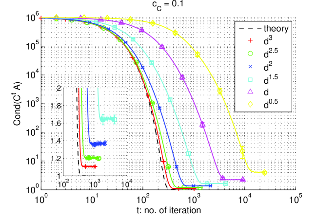
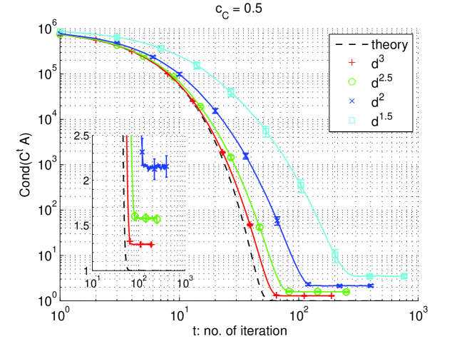
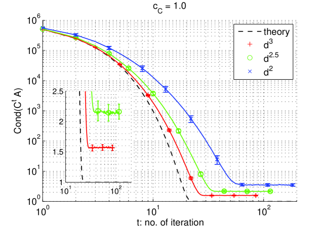
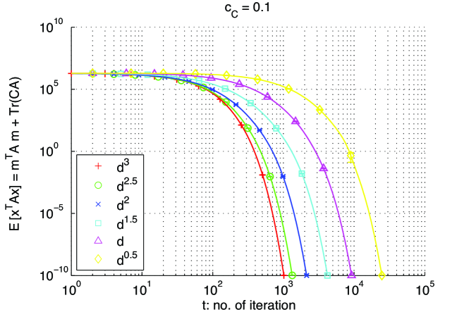
Figure 1: Averages and standard deviations of the condition numbers Cond(CtA)Condsuperscript𝐶𝑡𝐴\operatorname{Cond}(C^{t}A) for cC=0.1subscript𝑐𝐶0.1c_{C}=0.1, 0.50.50.5, and 1.01.01.0 and the expected objective function values for cC=0.1subscript𝑐𝐶0.1c_{C}=0.1. Theoretical curves (26) of the condition number are also illustrated with dashed lines. All the lines are cut after first reach of the expected objective value to 1010superscript101010^{-10}. Some results are omitted, for example n=d𝑛𝑑n=d for cC=0.5subscript𝑐𝐶0.5c_{C}=0.5, because numerically unstable computation occurs during search.

First, we investigate the effect of the sample size n𝑛n and the coefficient cCsubscript𝑐𝐶c_{C} of the learning rate ηCtsuperscriptsubscript𝜂𝐶𝑡\eta_{C}^{t}. We try the following sample sizes: d1/2superscript𝑑12\lceil d^{1/2}\rceil, d𝑑d, d3/2superscript𝑑32\lceil d^{3/2}\rceil, d2superscript𝑑2d^{2}, d5/2superscript𝑑52\lceil d^{5/2}\rceil, d3superscript𝑑3d^{3}.

Figure 1 illustrates the slope of the condition number Cond(CtA)Condsuperscript𝐶𝑡𝐴\operatorname{Cond}(C^{t}A) and the theoretical curve (26) and the slope of the expected objective function value 𝔼XPθt[XTAX]=(mt)TAmt+Tr(CtA)subscript𝔼similar-to𝑋subscript𝑃superscript𝜃𝑡delimited-[]superscript𝑋T𝐴𝑋superscriptsuperscript𝑚𝑡T𝐴superscript𝑚𝑡Trsuperscript𝐶𝑡𝐴\mathbb{E}_{X\sim P_{\theta^{t}}}[X^{\mathrm{T}}AX]=(m^{t})^{\mathrm{T}}Am^{t}+\operatorname{Tr}(C^{t}A), averaged over 505050 independent trials. When the sample size is larger, we see the closer performance to the theoretical result. When n=d3𝑛superscript𝑑3n=d^{3} and cC=0.1subscript𝑐𝐶0.1c_{C}=0.1, the convergence curve of the condition number approximated well the theoretical curve and the final condition number is Cond(CtA)1.1Condsuperscript𝐶𝑡𝐴1.1\operatorname{Cond}(C^{t}A)\approx 1.1. When n=d1/2𝑛superscript𝑑12n=\lceil d^{1/2}\rceil and cC=0.1subscript𝑐𝐶0.1c_{C}=0.1, it takes more than 303030 times longer to learn the covariance matrix and the final condition number becomes Cond(CtA)4.0Condsuperscript𝐶𝑡𝐴4.0\operatorname{Cond}(C^{t}A)\approx 4.0, although the stochastic algorithm still works successfully. We attain a little higher condition numbers when we choose larger learning rates cC=0.5subscript𝑐𝐶0.5c_{C}=0.5, 1.01.01.0. For example, the final condition numbers are Cond(CtA)1.3Condsuperscript𝐶𝑡𝐴1.3\operatorname{Cond}(C^{t}A)\approx 1.3 for n=d3𝑛superscript𝑑3n=d^{3} and cC=0.5subscript𝑐𝐶0.5c_{C}=0.5, and Cond(CtA)1.6Condsuperscript𝐶𝑡𝐴1.6\operatorname{Cond}(C^{t}A)\approx 1.6 for n=d3𝑛superscript𝑑3n=d^{3} and cC=1.0subscript𝑐𝐶1.0c_{C}=1.0. This is because smaller learning rates have more effect of averaging the natural gradient estimates over iterations and reducing the estimation variance.

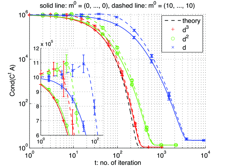
Note that we observe a slightly slower adaptation of the covariance matrix at the beginning in case that we set m0=(10,,10)superscript𝑚01010m^{0}=(10,\dots,10), although the adaptation behavior (26) does not change in theory. See Figure 2. This attributes to the estimation precision of Vf^^subscript𝑉𝑓\widehat{V_{f}}. If the squared Mahalanobis distance (mt)T(Ct)1mtsuperscriptsuperscript𝑚𝑡Tsuperscriptsuperscript𝐶𝑡1superscript𝑚𝑡(m^{t})^{\mathrm{T}}(C^{t})^{-1}m^{t} between the origin (the global optimum) and the current mean with respect to Ctsuperscript𝐶𝑡C^{t} is larger, the function landscape around mtsuperscript𝑚𝑡m^{t} looks more like linear function. Then Vf^(xi)^subscript𝑉𝑓subscript𝑥𝑖\widehat{V_{f}}(x_{i}) are far from the exact values, especially in case a small sample size is chosen.
Refer to caption
Figure 2: Averages and standard deviations of the change of the condition numbers for cC=0.1subscript𝑐𝐶0.1c_{C}=0.1 for n=d𝑛𝑑n=d, d2superscript𝑑2d^{2}, d3superscript𝑑3d^{3} with initial mean vector m=(0,,0)𝑚00m=(0,\dots,0) or m=(10,,10)𝑚1010m=(10,\dots,10). Other settings are the same as in Figure 1.

4.2 Comparison with Rank-μ𝜇\mu update CMA-ES

Finally, we study how well this stochastic algorithm simulates the CMA-ES. We test the pure rank-μ𝜇\mu update CMA-ES with weight scheme (9). We set the learning rates following [13]

ηmt=1,ηCt=2μw1(d+2)2+μw,formulae-sequencesuperscriptsubscript𝜂𝑚𝑡1superscriptsubscript𝜂𝐶𝑡2subscript𝜇𝑤1superscript𝑑22subscript𝜇𝑤\eta_{m}^{t}=1,\qquad\eta_{C}^{t}=\frac{2\mu_{w}-1}{(d+2)^{2}+\mu_{w}},

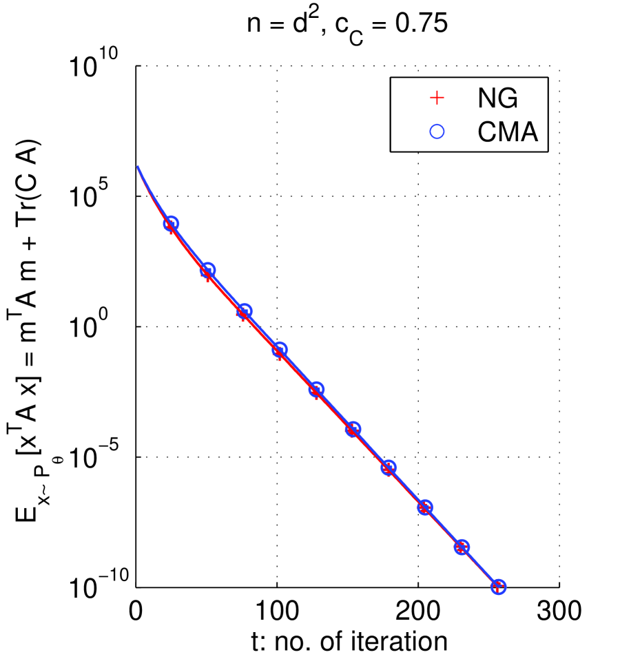
where μw=1/i=1nwi2subscript𝜇𝑤1superscriptsubscript𝑖1𝑛superscriptsubscript𝑤𝑖2\mu_{w}=1/\sum_{i=1}^{n}w_{i}^{2}. We choose cCsubscript𝑐𝐶c_{C} for our algorithm so that the speed of adaptation for each model is almost the same.

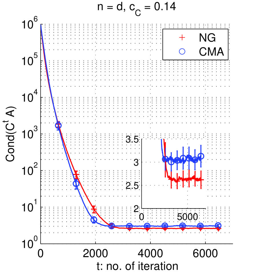
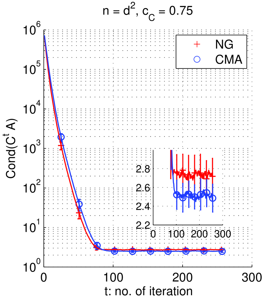
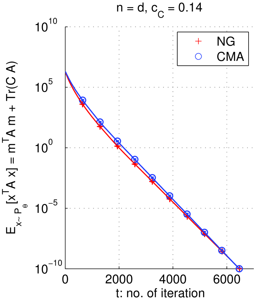
Figure 3 shows the results for each method for n=d𝑛𝑑n=d and n=d2𝑛superscript𝑑2n=d^{2}. In both case, we confirm similar behaviors of the pure rank-μ𝜇\mu update CMA-ES and our algorithm despite their dissimilar weight-value settings. The similar change of performance illustrated in Figure 2 is also observed for the pure rank-μ𝜇\mu update CMA-ES. From this result, we conclude that it is possible to estimate the performance of the pure rank-μ𝜇\mu update CMA-ES by our natural gradient algorithm, which is theoretically more attractive.

However, note that the pure rank-μ𝜇\mu update CMA-ES is not the standard CMA-ES [13] and the standard CMA-ES performs better than the pure rank-μ𝜇\mu update CMA-ES. The standard CMA-ES employes so-called evolution paths to adapt the covariance matrix and the global scale of the covariance matrix, which is called step-size in the CMA-ES context. Moreover, the standard CMA-ES employes weighted recombination, where different values are assigned to the weights for Rin/2subscript𝑅𝑖𝑛2R_{i}\leqslant\lfloor n/2\rfloor, which is only slightly better than intermediate recombination (9) and even similar to our setting. Furthermore, the similar performance observed is only on a quadratic function. If there are certain functions which distinguish our algorithm from the (rank-μ𝜇\mu) CMA-ES, this may help to understand both the NGD algorithm and the CMA-ES. Further study on these topics is required.
Refer to caption Refer to caption
Figure 3: Averages and standard deviations of the change of the condition numbers and the change of the expected objective function values for n=d𝑛𝑑n=d and cC=0.14subscript𝑐𝐶0.14c_{C}=0.14 on the left, and for n=d2𝑛superscript𝑑2n=d^{2} and cC=0.75subscript𝑐𝐶0.75c_{C}=0.75 on the right. Other settings are the same as in Figure 1.

5 Conclusion

We have proposed a novel natural gradient descent (NGD) method where the objective function is transformed to a function defined on the parameter space of probability distributions. We have proven that the deterministic NGD method learns the inverse of the Hessian of the original objective function that is any monotonic convex-quadratic-composite function. Linear convergence of the mean vector and the covariance matrix has been also proven. The numerical results for the stochastic NGD algorithm have shown that the stochastic algorithm approximates the deterministic one well when the sample size is sufficiently large. Moreover, we have confirmed that the stochastic NGD algorithm and the pure rank-μ𝜇\mu update CMA-ES behave very similarly on a quadratic function.

The contribution of the paper is to derive a novel NGD algorithm that can be viewed as a variant of the CMA-ES from the first principle of information geometry. This allows us to analyze the algorithm theoretically. Our theoretical results in Section 3 imply that there is at least one weight-value setting in the CMA-ES such that the covariance matrix learns the inverse of the Hessian of the objective function. Moreover, since our algorithm does not only share most of the important properties of the rank-μ𝜇\mu update CMA-ES, but also is confirmed to perform similarly to the pure rank-μ𝜇\mu update CMA-ES on a quadratic function by numerical simulations, we could study our algorithm to find out limitations of the pure rank-μ𝜇\mu update CMA-ES and to discover a way to improve the CMA-ES.

References

  • [1] Y. Akimoto, Y. Nagata, I. Ono, and S. Kobayashi. Bidirectional Relation between CMA Evolution Strategies and Natural Evolution Strategies. In Parallel Problem Solving from Nature – PPSN XI, pages 154–163, 2010.
  • [2] S. Amari. Natural Gradient Works Efficiently in Learning. Neural Computation, 10(2):251–276, 1998.
  • [3] S. Amari and H. Nagaoka. Methods of Information Geometry. Methods of Information Geometry. American Mathematical Society, 2007.
  • [4] S. Amari, H. Park, and K. Fukumizu. Adaptive method of realizing natural gradient learning for multilayer perceptrons. Neural Computation, 12:1399–1409, 2000.
  • [5] L. Arnold, A. Auger, N. Hansen, and Y. Ollivier. Information-Geometric Optimization Algorithms: A Unifying Picture via Invariance Principles. arXiv:1106.3708v1, 2011.
  • [6] A. Auger. Convergence results for the (111, λ𝜆\lambda)-SA-ES using the theory of φ𝜑\varphi-irreducible Markov chains. Theoretical Computer Science, 334(1-3):35–69, 2005.
  • [7] S. Baluja and R. Caruana. Removing the genetics from the standard genetic algorithm. In Proceedings of the 12th International Conference on Machine Learning, pages 38–46, 1995.
  • [8] S. Bhatnagar, R. S. Sutton, M. Ghavamzadeh, and M. Lee. Natural actor-critic algorithms. Automatica, 45(11):2471–2482, 2009.
  • [9] P. Billingsley. Probability and Measure. Wiley Series in Probability and Mathematical Statistics. Wiley-Interscience, third edition, 1995.
  • [10] P.-T. D. Boer, D. P. Kroese, S. Mannor, and R. Y. Rubinstein. A Tutorial on the Cross-Entropy Method. Annals of Operations Research, pages 19–67, 2005.
  • [11] T. Glasmachers, T. Schaul, S. Yi, D. Wierstra, and J. Schmidhuber. Exponential Natural Evolution Strategies. In Proceedings of Genetic and Evolutionary Computation Conference, pages 393–400. ACM, 2010.
  • [12] E. Greensmith, P. L. Bartlett, and J. Baxter. Variance Reduction Techniques for Gradient Estimates in Reinforcement Learning. Journal of Machine Learning Research, 5:1471–1530, 2004.
  • [13] N. Hansen and S. Kern. Evaluating the CMA Evolution Strategy on Multimodal Test Functions. In Parallel Problem Solving from Nature - PPSN VIII, pages 282–291, 2004.
  • [14] N. Hansen, S. D. Müller, and P. Koumoutsakos. Reducing the time complexity of the derandomized evolution strategy with covariance matrix adaptation (CMA-ES). Evolutionary Computation, 11(1):1–18, 2003.
  • [15] N. Hansen and A. Ostermeier. Completely derandomized self-adaptation in evolution strategies. Evolutionary Computation, 9(2):159–195, 2001.
  • [16] D. A. Harville. Matrix Algebra from a Statistician’s Perspective, Springer Verlag, 2008.
  • [17] J. Jägersküpper. Algorithmic analysis of a basic evolutionary algorithm for continuous optimization. Theoretical Computer Science, 379(3):329–347, 2007.
  • [18] P. Larrañaga and J. A. Lozano. Estimation of Distribution Algorithms: A New Tool for Evolutionary Computation, Springer Netherlands, 2002.
  • [19] L. Mirsky. A trace inequality of John von Neumann. Monatshefte für Mathematik, 79(4):303–306, 1975.
  • [20] J. Nocedal and S. J. Wright. Numerical Optimization. Springer Series in Operations Research. Springer, second edition, 2006.
  • [21] H. Park, S. Amari, and K. Fukumizu. Adaptive natural gradient learning algorithms for various stochastic models. Neural networks : the official journal of the International Neural Network Society, 13(7):755–764, 2000.
  • [22] J. Peters and S. Schaal. Natural actor-critic. Neurocomputing, 71(7-9):1180–1190, 2008.
  • [23] M. Rattray, D. Saad, and S. Amari. Natural gradient descent for on-line learning. Physical review letters, 81(24):5461–5464, 1998.