12 Years of Stellar Activity Observations in Argentina

Abstract

We present an observational program we started in 1999, to systematically obtain mid-resolution spectra of late-type stars, to study in particular chromospheric activity. In particular, we found cyclic activity in four dM stars, including Prox-Cen. We directly derived the conversion factor that translates the known $S$ index to flux in the Ca II cores, and extend its calibration to a wider spectral range. We investigated the relation between the activity measurements in the calcium and hydrogen lines, and found that the usual correlation observed is the product of the dependence of each flux on stellar color, and it is not always preserved when simultaneous observations of a particular star are considered. We also used our observations to model the chromospheres of stars of different spectral types and activity levels, and found that the integrated chromospheric radiative losses, normalized to the surface luminosity, show a unique trend for G and K dwarfs when plotted against the $S$ index.

1 Introduction

In 1999 we started a program to systematically obtain spectra of late-type stars, to study in particular chromospheric activity. The stars were chosen to cover the spectral range from F to M, with different activity levels. Since we were particularly interested in the transition to completely convective stars, we included a larger number of M stars in our sample.

Our observations were made at the 2.15 m telescope of the Complejo Astronómico El Leoncito (CASLEO), which is located at 2552 m above sea level, in San Juan, Argentina. We obtained high-resolution echelle spectra with a REOSC spectrograph. The maximum wavelength range of our observations is from 3860 to 6690 Å, and the spectral resolution ranges from 0.141 to 0.249 Å per pixel ($R=\lambda/\delta\lambda\approx 26400$).

At present, we have about 5500 spectra of 150 stars, ranging from F to M with different activity levels. Altough most of the stars are single dwarfs, we have several binaries and a few subgiants. Currently, we have four observing runs per year. Details on the reduction and calibration procedures can be found in [Cincunegui & Mauas 2004, Cincunegui & Mauas (2004)].

2 Flux-Flux calibrations

Since, unlike most surveys of this kind, the observations in the different spectral features are made simultaneously, our data provides an excellent opportunity to study the correlation between different spectral features and activity indexes. To date, the most common indicator of chromospheric activity is the well-known $S$ index, essentially the ratio of the flux in the core of the Ca II H and K lines to the continuum nearby ([Vaughan et al. 1978]). This index has been defined at the Mount Wilson Observatory, were an extensive database of stellar activity has been built over the last four decades. However, unlike our program, these observations are mainly concentrated on stars ranging from F to K, due to the long exposure times needed to observe the Ca II lines in the red in faint M stars. For this reason, the $S$ index is poorly characterized for these stars. We first obtained the $S$ index for our spectra, integrating with the corresponding profile (for details, see [Cincunegui, Díaz & Mauas 2007a]).

The Mount Wilson $S$ index can be converted to the average surface flux in the Ca II lines through the relation:

$$F_{\mathrm{HK}}=F_{\mathrm{bol}}1.34\,10^{-4}\,S\,C_{\mathrm{cf}}\,,$$ (1)

where $C_{\mathrm{cf}}\left(B\!-\!V\right)$ is a conversion factor that depends on color. Two different expressions are widely used for this factor, the first one given by [Middelkoop (1982)] and corrected by [Noyes et al. (1984)] and the other one given by [Rutten (1984)]. The deductions used in both works to derive $C_{\mathrm{cf}}$ involve complex calibration procedures.

Since we have simultaneous measurements of the $S$ index and the core fluxes, we can calculate directly the correction factor as a function of the index and the flux, which is shown in Fig. 1 together with the other two expressions (for details and a whole discussion, see [Cincunegui, Díaz & Mauas 2007a]).

Figure 1: Conversion factor between Mount Wilson $S$ index and $F_{\mathrm{HK}}$. The dashed line corresponds to [Noyes et al. (1984)], the dotted line to [Rutten (1984)], and the full line to our derived factor (from [Cincunegui, Díaz & Mauas 2007a]).

It is usually accepted that there is a tight relation between the chromospheric fluxes emitted in H-$\alpha$ and in the H and K Ca II lines, and that these two features can be used to study chromospheric activity. However, most works where this relation has been observed found it by using averaged fluxes for both the calcium and the hydrogen lines, which were not obtained simultaneously, and were even collected from different sources.

However, the situation is different when the individual stars are studied separately. In Fig. 2 we plot the individual simultaneous measurements of each flux for several stars of different spectral types and different levels of activity, divided into color bins as stated. We also show the linear fits for each star. It can be seen that the behavior is different in each case: in some stars both fluxes are well correlated, although the slopes of the fits are not the same. In other stars the H-$\alpha$ flux seems to be almost independent of the level of activity measured in the Ca II lines, and there are even stars where the fluxes are anti-correlated.

Figure 2: H-$\alpha$ vs. Ca II surface fluxes, for stars of different spectral types, divided into different color bins, as indicated (from [Cincunegui, Díaz & Mauas 2007a]).

In [Díaz, Cincunegui & Mauas (2007)] we studied the sodium D lines (D1: 5895.92 Å; D2: 5889.95 Å) in our stellar sample. We found a good correlation between the equivalent width of the D lines and the color index $(B-V)$ for all the range of observations. Since equivalent width is a characteristic of line profiles that do not require high resolution spectra to be measured, this fact could become a useful tool for subsequent studies. Finally, we constructed a spectral index ($R^{\prime}_{D}$) as the ratio between the flux in the D lines and the bolometric flux. Once corrected for the photospheric contribution, this index can be used as a chromospheric activity indicator in stars with a high level of activity. Additionally, we found that combining some of our results, we obtained a method to calibrate in flux stars of unknown color.

3 Cycles in M-stars

One of the main goals of our program was to extend the studies of stellar cycles to M-stars, at and beyond the limit for full convectivity. The first star we studied was Proxima Centaury, a dMe 5.5 star with strong and frequent flaring activity [Cincunegui, Díaz & Mauas 2007b, Cincunegui, Díaz & Mauas (2007b)]. For this star we excluded the spectra taken during flares, computed the nightly average of the H$\alpha$ flux, and calculated the Lomb-Scargle periodogram, which is shown in Fig. 3. In the periodogram we found strong evidence of a cyclic activity with a period of $\sim$442 days. Similar values for the period were found using three different techniques in the time domain (see [Cincunegui, Díaz & Mauas 2007b] for details). We were also able to determine that the activity variations outside of flares amount to 130% in $S$, three times larger than for the Sun.

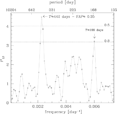
Figure 3: Lomb-Scargle periodogram of our observations. The False Alarm Probability levels of 50 and 80% are shown. (from [Cincunegui, Díaz & Mauas 2007b]).

Since this star should be fully convective, it cannot support an $\alpha\Omega$ dynamo, and a different mechanism should be found to explain this result. Recently, [Chabrier & Küker (2006)] showed that these objects can support large-scale magnetic fields by a pure $\alpha^{2}$ dynamo process. Moreover, these fields can produce the high levels of activity observed in M stars (see, for example, [Mauas & Falchi 1996]. This $\alpha^{2}$ dynamo does not predict a cyclic activity. However, our observations suggest that this cool star has a clear period.

We also studied the spectroscopic binary system Gl 375 ([Díaz, González, Cincunegui, Mauas 2007]). We first obtained precise measurements of the orbital period (P = 1.87844 days) and separation (a = 5.665 $\mathrm{R_{\odot}}$), minimum masses and other orbital parameters. We separated the composite spectra into those corresponding to each component, which allows us to confirm that both components are of spectral type dMe 3.5.

To study the variability of Gl 375, besides using the spectra obtained at CASLEO, we also employed photometric observations provided by the All Sky Automated Survey (ASAS [Pojmanski 2002]). We calculated the Lomb-Scargle periodogram for these data, and obtained a a distinct peak corresponding to a period of $\mathrm{P_{phot}}=1.876667$ days, a period resembling very closely the measured orbital period. We believe this harmonic variability is produced by spots and active regions in the stellar surface carried along with rotation. This would imply that the rotational and orbital periods are synchronized, as is expected for such a close binary.

To verify if this is indeed the case, we phased the data to the obtained period, for two different seasons (Fig. 4). The sinusoidal shape of the variation is evident, although the amplitude of the modulation is different in both cases, probably an indication of different area covered by starspots or active regions, and therefore different activity levels, in each epoch. Therefore, the amplitude of this modulation can be used as an activity proxy, and indicates that the system exhibits a roughly periodic behavior of 2.2 years (or ∼800 days). The same period was found in the mean magnitude of the system and in the flux of the Ca II K line, although the Ca flux variations occur 140 days ahead of the photometric ones, a behavior that has been previously observed in other stars ([Gray et al. 1996]). The agreement between the behavior of the three observables is remarkable because of the different nature of the observations and the different instruments and sites where they were obtained.

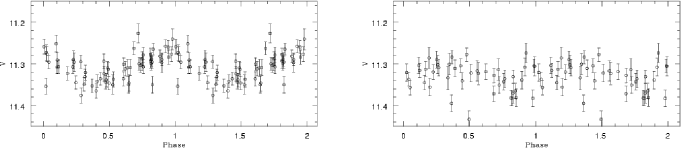
Figure 4: ASAS photometry phased to the orbital period for two different epochs. Left: 2002.5-2003.5 Right: 2006. (from [Díaz, González, Cincunegui, Mauas 2007]).

Another interesting result of this work is that the activity of Gl 375 A and Gl 375 B, as measured in the flux of the Ca II K lines, are in phase, as can be seen in Fig. 5. There is an excellent correlation between the levels of chromospheric emission of both components, implying a magnetic connection between them. Due to its vicinity and relative brightness, this system presents an interesting opportunity to further study this type of interaction.

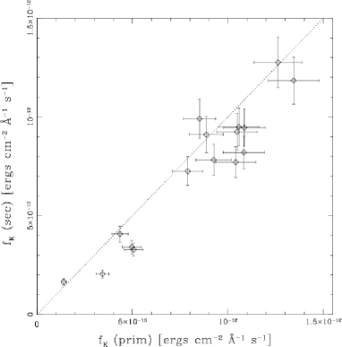
Figure 5: Comparison of the fluxes in the Ca II K line for both components. The error bars correspond to a 10% error in the line fluxes, and the dotted line is the identity relation. (from [Díaz, González, Cincunegui, Mauas 2007]).

We also studied the long-term activity of two other M dwarf stars: Gl 229 A and Gl 752 A, using again the Ca II - K line-core fluxes measured on our spectra and the ASAS photometric data. Using the Lomb-Scargle periodogram, we obtained a possible activity cycle of $\sim$4 and $\sim$7 yrs for Gl 229 A and Gl 752 A, respectively ([Buccino et al. 2011]). This work was complemented by other studies, were we investigated the presence of activity cycles using IUE data ([Buccino & Mauas 2008] and [Buccino & Mauas 2009]).

4 Chromospheric modeling

We also used our spectra as observational basis to model the chromosphere of different type of stars ans activity levels, following the path initiated with the model of Ad-Leonis in its quiescent state ([Mauas & Falchi 1994]), which was completed with a study of other dM 3.5 stars of different activity levels ([Mauas et al 1997]). We first computed models of the Sun as a star and 9 solar analogues ([Vieytes, Mauas & Cincunegui (2005), Vieytes, Mauas & Cincunegui 2005]) which were followed by models for 6 K stars, “analogs” of epsilon-Eridani ([Vieytes, Díaz & Mauas (2009), Vieytes, Díaz & Mauas 2009]). For most stars, we built two models, to match the observations in its minimum and maximum levels of activity, and found that the differences in the atmospheric structure for a star in its maximum and minimum activity levels are similar to the changes seen between two different stars.

We also found that the integrated chromospheric radiative losses $\phi_{\mathrm{{int}}}$, normalized to the surface luminosity, show a unique trend for G and K dwarfs when plotted against the $S$ index, (see Fig. 6). This might indicate that the same physical processes are heating the stellar chromospheres in both cases. We calculated an empirical relationship between $S$ and the energy deposited in the chromosphere, which can be used to estimate the energetic requirements of a given star knowing its chromospheric activity level.

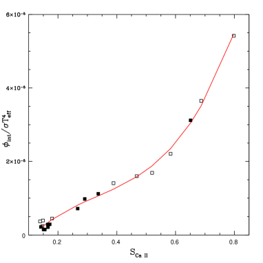
Figure 6: Normalized $\phi_{\mathrm{{int}}}$ versus the $S$ index. The squares represent the K star models from [Vieytes, Díaz & Mauas (2009)] and the triangles indicate the G star models from [Vieytes, Mauas & Cincunegui (2005)].

STEVE SAAR You mentioned ASAS data in a couple of cases, I would encourage you to look at the ASAS data for Proxima Centauri. By an odd coincidence we have been looking for an x-ray cycle in that recently and it has what appears to be a good photometric period but it is more like 8 years rather than the period you quote here. I have been wondering if you see a signal in that range.

PABLO MAUAS I was thinking it was time for an update in that star, since we have four more years of data and we certainly have to use the ASAS data. We will have a look at it.

JURGEN SCHMITT Alpha Cen must be perfectly suited for observations you have – have you looked at Alpha Cen?

PABLO MAUAS Yes, we have, but we had a problem with the gain of the pointing screen at the observatory so we had to end those observations three or four years ago. But we have a hint of a cycle in the K-star, Alpha Cen B.

MARK GIAMPAPA I think it is great that you are getting cycle periods for M dwarf stars. Just a comment on the H-$\alpha$ and Calcium K. The models that I have constructed and looked at show that they are very segregated in their formation regions and so you could have some, at least in models, disjoint behavior, but I am surprised that you don’t see in observations pretty direct correlation. But, in any event I could imagine in the upper atmosphere you could have flare-like behavior that may not propagate into the lower atmosphere and that could lead to some deep correlation between Calcium and H $\alpha$.

PABLO MAUAS Flare activity we usually can detect because we take two spectra to eliminate cosmic rays, so before we do anything with our data we check to see if the spectra are more or less the same. So if you had a flare, that wouldn’t happen particularly not for M stars integration times are very long. So usually we leave out all the flares. For Proxima for example that’s hard work because you can have four or five flares a day. So usually those extremes are eliminated from our data. I think there can be different things for these different correlations between Calcium and H-$\alpha$. One can be filling factor problems. Perhaps you can explain the same integrated emission with different filling factors and different contrasts but they won’t give the same relation between H-$\alpha$ and Calcium. The other one is the orientation - it is not the same if you observe the star pole-on or from the equator. So we are exploring that, and preliminary results are shown in our poster.

References

- [Buccino et al. 2011] Buccino, A. P.; Díaz, R. F.; Luoni, M. L.; Abrevaya, X. C. & Mauas, P. J. D. 2011, AJ 141, 34
- [Buccino & Mauas 2008] Buccino, A. P. & Mauas, P. J. D. 2008, 483, 903
- [Buccino & Mauas 2009] Buccino, A. P. & Mauas, P. J. D. 2008, 495, 287
- [Chabrier & Küker (2006)] Chabrier, G. & Küker, M. 2006, A&A 446, 1027
- [Cincunegui & Mauas 2004] Cincunegui, C.C., & Mauas, P.J.D. 2004, A&A, 414, 699
- [Cincunegui, Díaz & Mauas 2007a] Cincunegui, C.C., Díaz, R. & Mauas, P.J.D. 2007a, A&A, 469, 309
- [Cincunegui, Díaz & Mauas 2007b] Cincunegui, C.C., Díaz, R. & Mauas, P.J.D. 2007b, A&A, 461, 1107
- [Díaz, Cincunegui & Mauas (2007)] Díaz, R., Cincunegui, C.C. & Mauas, P.J.D. 2007, MNRAS, 378, 1007
- [Díaz, González, Cincunegui, Mauas 2007] Díaz, R., González, F., Cincunegui, C.C. & Mauas, P.J.D. 2007, A&A, 474, 345
- [Gray et al. 1996] Gray, D. F., Baliunas, S. L., Lockwood, G. W., & Skiff, B. A. 1996, ApJ, 465, 945
- [Mauas & Falchi 1994] Mauas, P. J. D.; Falchi, A. 1994, A&A 281, 129
- [Mauas & Falchi 1996] Mauas, P. J. D. & Falchi, A. 1996, A&A, 310, 245
- [Mauas et al 1997] Mauas, P. J. D.; Falchi, A.; Pasquini, L.& Pallavicini, R. 1997, A&A 326, 249
- [Middelkoop (1982)] Middelkoop, F. 1982, A&A 107, 31
- [Noyes et al. (1984)] Noyes, R. W., Hartmann, L. W., Baliunas, S. L., Duncan, D. K., & Vaughan, A. H. 1984, ApJ 279, 763
- [Pojmanski 2002] Pojmanski, G. 2002, Acta Astron. 52, 397
- [Rutten (1984)] Rutten, R. G. M. 1984, A&A 130, 353
- [Vaughan et al. 1978] Vaughan, A.H., Preston, G.W. & Wilson, O.C. 1978, PASP 90, 267
- [Vieytes, Mauas & Cincunegui (2005)] Vieytes, M.; Mauas, P. J. D. & Cincunegui, C. C. 2005, A&A 441, 701
- [Vieytes, Díaz & Mauas (2009)] Vieytes,M.; Díaz, R. & Mauas, P. J. D. 2009, MNRAS 398, 1495.