Anomalous Surface Impedance in a Normal-metal/Superconductor Junction with a Spin-active Interface

Abstract

We discuss the surface impedance ($Z=R-iX$) of a normal-metal/superconductor proximity structure taking into account the spin-dependent potential at the junction interface. Because of the spin mixing transport at the interface, odd-frequency spin-triplet $s$-wave Cooper pairs penetrate into the normal metal and cause the anomalous response to electromagnetic fields. At low temperature, the local impedance at a surface of the normal metal shows the nonmonotonic temperature dependence and the anomalous relation $R>X$. We also discuss a possibility of observing such anomalous impedance in experiments.

I introduction

Physics of odd-frequency Cooper pairsberezinskii has been a hot issue since a theoretical paper pointed out the existence of odd-frequency pairs in realistic proximity structures bergeret . There are mainly two ways to create the odd-frequency Cooper pairs in proximity structures. At first, spin-mixing due to spin-dependent potential should generate odd-frequency pairs. The authors of Ref. bergeret, considered a ferromagnet / metallic-superconductor junction, where the direction of magnetic moment near the interface is spatially inhomogeneous. The spin-flip scattering in such magnetically inhomogeneous segment produces the odd-frequency spin-triplet $s$-wave Cooper pairs in the ferromagnet. This prediction has promoted a number of theoretical studies ya07sfs ; braude ; eschrig ; linder ; fominov1 ; yokoyama0 ; yokoyama ; halterman . Manifestations of triplet pairs were recently observed experimentally as a long-range Josephson coupling across ferromagnets Keizer ; Anwar ; Robinson ; Khaire . Alternatively, the odd-frequency pair was suggested in proximity structures involving a normal metal attached to an odd-parity spin-triplet superconductor that belongs to the conventional even-frequency symmetry class. The parity-mixing due to inhomogeneity produces the odd-frequency pairs even in this case tanaka07e . The unusual properties of spin-triplet superconducting junctions due to odd-frequency pairs tanaka07L ; yt04 ; yt05r ; ya06 ; ya07 ; fominov2 were predicted theoretically. Unfortunately, however, we have never had clear scientific evidences of odd-frequency pairs in experiments. This is because physical values focused in experiments have only indirect information of the frequency symmetry.

In a previous paper ya11 , we showed that the surface impedance directly reflects the frequency symmetry of Cooper pair. Surface impedance $Z=R-iX$ represents the dynamic response of Cooper pairs to low frequency electromagnetic field mattice ; nam . The surface resistance, $R$, corresponds to resistance due to normal electrons. The reactance, $X$, represents power loss of electromagnetic field due to Cooper pairs. In conventional even-frequency superconductors, the positive amplitude of the Cooper pair density guarantees a robust relation $R\ll X$ at low temperatures and at low frequencies. The validity of the relation $R<X$, however, is questionable for odd-frequency Cooper pairs because the odd-frequency symmetry and negative pair density are inseparable from each other according to the standard theory of superconductivity agd . We have considered a a normal metal/superconductor (NS) junction where superconductor belongs to spin-triplet odd-parity symmetry. We have theoretically shown that the odd-frequency Cooper pairs in the normal metal lead to the unusual relationship $R>X$. Therefore observing the relation $R>X$ in experiments can be a very clear and direct evidence which suggests the existence of odd-frequency Cooper pairs. Although the detection of such unusual relation is possible these days, the fabrication of a well characterized NS junction using chiral $p$-wave spin-triplet superconductor Sr₂RuO₄ maeno is not easy task. Thus we need to discuss a possibility for observing the unusual relationship $R>X$ in another accessible proximity structures.

In this paper, we discuss the surface impedance in NS junction consisting of a metallic superconductor where pairing symmetry belongs to spin-singlet $s$-wave. At the junction interface, we introduce a thin ferromagnetic layer which produces the odd-frequency spin-triplet $s$-wave Cooper pairs in the normal metal. The local complex conductivity is calculated based on the linear response theory using the quasiclassical Green function method. We will conclude that the local impedance in the normal metal show the unusual relation $R>X$ when the odd-frequency pairs is dominant in the normal metal. We also discuss a possibility to detect of the relation in experiments.

This paper is organized as follows. In Sec. II, we explain the theoretical model of a NS junction and the formula for complex conductivity. The calculated results of impedance in NS junctions are shown in Sec. III. The conclusion is given in Sec. IV.

II Model and Method

Let us consider a bilayer of a superconductor and a thin normal metal film as shown in Fig. 1, where $L$ is the thickness of the normal metal.

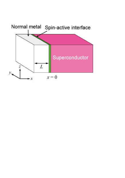
Figure 1: (color online). The schematic picture of a normal-metal/superconductor junction under consideration.

To calculate the complex conductivity in the normal metal, we first solve the quasiclassical Usadel equation usadel in the standard $\theta$-parameterization,

$$\hbar D\frac{d^{2}\theta_{\nu}(x,\epsilon)}{dx^{2}}+2i\epsilon\sin\theta_{\nu}(x,\epsilon)=0,$$ (1)

where $D$ is the diffusion constant of the normal metal and $\epsilon$ is the quasiparticle energy measured from the Fermi level. The subscript $\nu=\pm 1$ describes two Nambu spaces: $\nu=1$ indicates the subspace for electron spin-up and hole spin-down, and $\nu=-1$ indicates that for electron spin-down and hole spin-up. Effects of spin-dependent scatterings are considered through the boundary condition at the NS interface kupriyanov ; daniel ; cottet ; linder ; yoshizaki ,

$$\gamma_{B}\left.\frac{d\theta_{\nu}}{dx}\right|_{x=0}=\sin(\theta_{\nu}-\theta_{S})+i\nu\frac{G_{\phi}}{G_{T}}\sin\theta_{\nu},$$ (2)

where $\gamma_{B}=L\frac{R_{b}}{R_{d}}$ is a interface parameter with $R_{d}$ and $R_{b}$ being the resistance of the normal metal and that of the NS interface, respectively. The Green function in superconductor is described by

$$g_{S}=\cos\theta_{S}= \frac{\epsilon}{\sqrt{(\epsilon+i\lambda)^{2}-\Delta}},$$ (3)

$$f_{S}=\sin\theta_{S}= \frac{i\Delta}{\sqrt{(\epsilon+i\lambda)^{2}-\Delta}},$$ (4)

where $\Delta$ is the amplitude of pair potential in the bulk superconductor and $\lambda$ is a small parameter providing the retarded Green function. The second term in Eq. (2) describes the spin-mixing effect at the junction interface. $G_{T}$ represents the spin-independent tunneling conductance of the junction interface, whereas $G_{\phi}$ is the spin-mixing conductance yokoyama3 . At the outer surface of the normal metal, we require

$$\left.\frac{\partial\theta(x,\epsilon)}{\partial x}\right|_{x=-L}=0.$$ (5)

The normal and anomalous retarded Green functions are obtained as

$$g_{\nu}(x,\epsilon)=\cos\theta_{\nu}(x,\epsilon),\;f_{\nu}(x,\epsilon)=\sin\theta_{\nu}(x,\epsilon),$$ (6)

respectively.

Having found the Green functions, we can calculate the local complex conductivity that describes the response of the sample to the electromagnetic field. The local complex conductivity $\sigma_{\textrm{N}}(x,\omega)=\sigma_{1}+i\sigma_{2}$ at frequency $\omega$ is determined by the general expression FGH

$$\frac{\sigma_{1}(x,\omega)}{\sigma_{0}} =\frac{1}{2\hbar\omega}\int_{-\infty}^{\infty}\!\!\!\!\!\!d\epsilon\left[J(\epsilon+\hbar\omega)-J(\epsilon)\right]K_{1},$$ (7)

$$\frac{\sigma_{2}(x,\omega)}{\sigma_{0}} =\frac{1}{2\hbar\omega}\int_{-\infty}^{\infty}\!\!\!\!\!\!d\epsilon\left[J(\epsilon+\hbar\omega)K_{2}+J(\epsilon)K_{3}\right],$$ (8)

$$K_{1}=\sum_{\nu}f_{\nu,I} (\epsilon)f_{\nu,I}(\epsilon+\hbar\omega)\!+\!g_{\nu,R}(\epsilon)g_{\nu,R}(\epsilon+\hbar\omega),$$ (9)

$$K_{2}=\!\sum_{\nu}f_{\nu,R} (\epsilon)f_{\nu,I}(\epsilon+\hbar\omega)\!-\!g_{\nu,I}(\epsilon)g_{\nu,R}(\epsilon+\hbar\omega),$$ (10)

$$K_{3}=\!\sum_{\nu}f_{\nu,R} (\epsilon+\hbar\omega)f_{\nu,I}(\epsilon)\!-\!g_{\nu,I}(\epsilon+\hbar\omega)g_{\nu,R}(\epsilon),$$ (11)

with $J(\epsilon)=\tanh\left({\epsilon}/{2k_{B}T}\right)$ and

$$g_{\nu,R}(\epsilon)= \mathop{\mathrm{missing}}{Re}\nolimits\left[g_{\nu}(x,\epsilon)\right],\;g_{\nu,I}(\epsilon)=\mathop{\mathrm{missing}}{Im}\nolimits\left[g_{\nu}(x,\epsilon)\right],$$ (12)

$$f_{\nu,R}(\epsilon)= \mathop{\mathrm{missing}}{Re}\nolimits\left[f_{\nu}(x,\epsilon)\right],\;f_{\nu,I}(\epsilon)=\mathop{\mathrm{missing}}{Im}\nolimits\left[f_{\nu}(x,\epsilon)\right].$$ (13)

The local impedance in the normal metal is calculated from the complex conductivity as

$$Z_{\textrm{N}}(x,\omega)=R_{\textrm{N}}-iX_{\textrm{N}}=(1-i)\sqrt{\frac{\hbar\omega}{\Delta_{0}}\frac{\sigma_{0}}{\sigma_{\textrm{N}}(x,\omega)}}{Z_{\textrm{0}}},$$ (14)

where $Z_{\textrm{0}}\equiv\sqrt{2\pi\Delta_{0}/\sigma_{0}c^{2}\hbar}$, $\Delta_{0}$ is the amplitude of pair potential at $T=0$, and $\sigma_{0}$ is the Drude conductivity in the normal metal. In this paper, we describe the dependence of $\Delta$ on temperature by the BCS theory. In particular, we focus on the local impedance at the surface of the normal metal defined by

$$R_{L}-iX_{L}\equiv Z_{\textrm{N}}(-L,\omega).$$ (15)

Such local impedance is an accessible observable these days machida . Usual experiments measure the impedance of the whole NS structure which is calculated as

$$Z_{\textrm{NS}}= R_{\textrm{NS}}\!-\!iX_{\textrm{NS}}=\bar{Z}_{\textrm{N}}\frac{Z_{\textrm{S}}\cos\bar{k}_{n}L\!-\!i\bar{Z}_{\textrm{N}}\sin\bar{k}_{n}L}{\bar{Z}_{\textrm{N}}\cos\bar{k}_{n}L\!-\!iZ_{\textrm{S}}\sin\bar{k}_{n}L},$$ (16)

where $Z_{S}$ is the impedance of superconductor which is obtained by substituting the Green function of superconductor in Eqs. (3)-(4) into Eqs. (7)-(13). In this paper, $L$ is chosen to be comparable to $\xi_{T_{c}}=\sqrt{\hbar D/2\pi T_{C}}$ with $T_{C}$ is the superconducting transition temperature. In such junctions, the conductivity is almost independent of $x$ in the normal metal. Therefore it is possible to define spatially averaged values of the conductivity, the impedance and the wavenumber of electromagnetic field as follows

$$\bar{\sigma}_{\textrm{N}}= \int_{-L}^{0}dx\sigma_{\textrm{N}}(x)/L,$$ (17)

$$\bar{Z}_{\textrm{N}}= \bar{R}_{\textrm{N}}-i\bar{X}_{\textrm{N}}=-i\sqrt{4\pi i\omega/(c^{2}\bar{\sigma}_{\textrm{N}})},$$ (18)

$$\bar{k}_{n}= \sqrt{i{4\pi\omega\bar{\sigma}_{\textrm{N}}}/{c^{2}}}.$$ (19)

To understand the relation between the frequency symmetry of a Cooper pair and the sign of the imaginary part of complex conductivity $\sigma_{2}$, we analyze the spectral pair density defined by

$$K_{s}(\epsilon)= \sum_{\nu}f_{\nu,R}(\epsilon)f_{\nu,I}(\epsilon)-g_{\nu,R}(\epsilon)g_{\nu,I}(\epsilon),$$ (20)

$$= \sum_{\nu}2f_{\nu,R}(\epsilon)f_{\nu,I}(\epsilon)=\sum_{\nu}\textrm{Im}f_{\nu}^{2}(\epsilon),$$ (21)

which appears in the integrand of $\sigma_{2}$ in Eq. (8) at very small $\omega$. We used the normalization condition $g_{\nu}^{2}(\epsilon)+f_{\nu}^{2}(\epsilon)=1$. The spectral pair density contains full information about the symmetry of $f(\epsilon)$ and, therefore, the frequency symmetry of Cooper pairs. At $T=0$, the Cooper pair density in the normal metal is

$$n_{s}=\int_{-\infty}^{\infty}d\epsilon J(\epsilon)K_{s}(\epsilon).$$ (22)

Since $K_{s}$ is an odd function of $\epsilon$ according to its definition and $J(\epsilon)$ is also odd step function of $\epsilon$, the pair density becomes

$$n_{s}=2\int_{0}^{\infty}d\epsilon K_{s}(\epsilon).$$ (23)

Finally the local density of states is given by

$$N(\epsilon,x)=\sum_{\nu}\textrm{Re}[g_{\nu}(\epsilon,x)],$$ (24)

which is normalized to the normal density of states at the Fermi level.

III Results

The theory includes several independent parameters discussed as follows. Throughout this paper, we fix the thickness of a normal metal $L$ at $\xi_{T_{c}}$. The spatial dependence of the Green function in the normal metal becomes weak in this choice. In numerical simulation, we do not discuss details of the averaged impedance $\bar{Z}_{\text{N}}$ in Eq. (18) because we have confirmed that $Z_{L}\approx\bar{Z}_{\text{N}}$. The second parameter $R_{d}/R_{b}$ tunes the degree of the proximity effect in a normal metal. The larger $R_{d}/R_{b}$ gives the stronger proximity effect. The third one is $G_{\phi}/G_{T}$ which represents the strength of spin-dependent potential at the NS interface. The forth one is the frequency of electromagnetic field $\omega$ which should be smaller than $\Delta_{0}/\hbar$ to obtain information about Cooper pairs. Finally we fix the small imaginary part in energy as $\lambda=0.001\Delta_{0}$, which does not affect following conclusions.

III.1 Density of States

We first show the local density of states (LDOS) at a surface of the normal metal for several choices of $G_{\phi}/G_{T}$ in Fig. 2. Here we choose the parameter $R_{d}/R_{b}=0.2$, which means the proximity effect is weak.

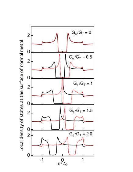
Figure 2: (color online). Local density of states at the surface of the normal metal with $R_{d}/R_{b}=0.2$. The results for $\nu=1$ and $\nu=-1$ are shown with the solid and broken lines, respectively.

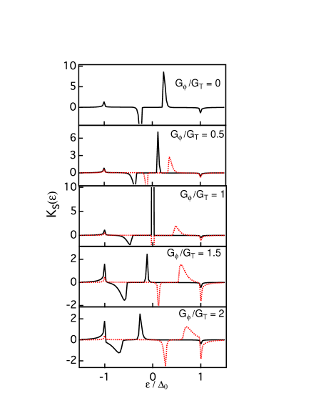
Figure 3: (color online). $K_{s}$ function at the surface of the normal metal. The local pair density is calculated from Eq. (23).

The solid and broken lines are the results calculated for $\nu=1$ and -1, respectively. At $G_{\phi}/G_{T}=0$, two LDOS for $\nu=\pm 1$ are identical to each other and show the minigap structure for $|\epsilon|\leq 0.2\Delta_{0}$ due to the proximity effect. In Fig. 3, we show the pair spectral density defined in Eq. (21). At $G_{\phi}/G_{T}=0$, $K_{s}$ has a large positive peak around $\epsilon\approx 0.2\Delta_{0}$. Therefore the local pair density in Eq. (23) becomes positive. This means the penetration of even-frequency pairs into the normal metal. When we introduce $G_{\phi}/G_{T}$ at 0.5, LDOS for $\nu=1$ shifts to negative direction, whereas that for $\nu=-1$ moves to positive direction. Correspondingly large positive peaks in $K_{s}$ are separated into two as shown in Fig. 3. At $G_{\phi}/G_{T}=1.0$, two peaks in LDOS overlap each other. In $K_{s}$ function, the large positive peak for $\nu=1$ totally cancels the large negative peak for $\nu=-1$. As discussed in a previous paper linder , $G_{\phi}/G_{T}=1.0$ is a critical value. For $G_{\phi}/G_{T}<1.0$, the even-frequency Cooper pairs is dominant in the normal metal. On the other hand for $G_{\phi}/G_{T}>1.0$, the fraction of odd-frequency Cooper pair increases with increasing $G_{\phi}/G_{T}$. In particular at $\epsilon=0$, the frequency symmetry of Cooper pairs is purely odd. When we increase $G_{\phi}/G_{T}=$ 1.5 and 2.0, the minigap in two subspaces are separated from each other as shown in Fig. 2. At the same time, $K_{s}$ has a large negative peak in low energy region, which means the penetration of odd-frequency Cooper pairs into the normal metal.

III.2 Impedance

Next we show the impedance as a function of temperature for several choices of $G_{\phi}/G_{T}$ in Fig. 4, where $\hbar\omega=0.1\Delta_{0}$. We choose a boundary parameter as $R_{d}/R_{b}=0.2$ in Fig. 4, which again means the proximity effect is weak. The results for $G_{\phi}/G_{T}=0$ in Fig. 4(a) shows the typical and conventional behavior of impedance in NS junctions. The local impedance at the surface of normal metal $R_{\textrm{L}}$ and $X_{\textrm{L}}$ monotonically decrease with decreasing temperature far below $T_{C}$ and satisfy the robust relation $R_{\textrm{L}}<X_{\textrm{L}}$. The impedance of a NS bilayer $R_{\textrm{NS}}$ and $X_{\textrm{NS}}$ show qualitatively similar behavior. Namely the impedance satisfies $R_{\textrm{NS}}<X_{\textrm{NS}}$. These behavior are a direct consequence of the fact that all Cooper pairs belong to even-frequency spin-singlet $s$-wave pairing symmetry. Such characteristic feature remains even if we introduce $G_{\phi}/G_{T}$ by small amount up to 1.0 as shown in Fig. 4(b). In the presence of the spin-dependent potential at the NS interface, the odd-frequency spin-triplet $s$-wave Cooper pairs appear in the normal metal in addition to conventional even-frequency spin-singlet $s$-wave pairs. The fraction of odd-frequency pairs is much smaller than that of even-frequency pairs for $G_{\phi}/G_{T}\leq 1$. However $G_{\phi}/G_{T}$ exceeds unity as shown in Figs. 4(c) and (d), the the local impedance shows the unusual relation $R_{\textrm{L}}>X_{\textrm{L}}$ at low temperature for $T<T^{\ast}$, where $T^{\ast}$ is defined as the crossover temperature. In Figs. 4(c) and (d), $T^{\ast}$ is about 0.02 for $G_{\phi}/G_{T}=1.5$ and is 0.06 for $G_{\phi}/G_{T}=2$, respectively. At the same time, $R_{\textrm{NS}}$ and $X_{\textrm{NS}}$ show the nonmonotonic dependence of temperature for $T<T^{\ast}$. For $G_{\phi}/G_{T}\geq 1$, the fraction of the odd-frequency Cooper pairs become becomes larger than that of the even-frequency pairs. Thus the anomalous behavior of impedance in Figs. 4(c) and (d) is the direct evidence of the odd-frequency Cooper pairs in the normal metal ya11 .

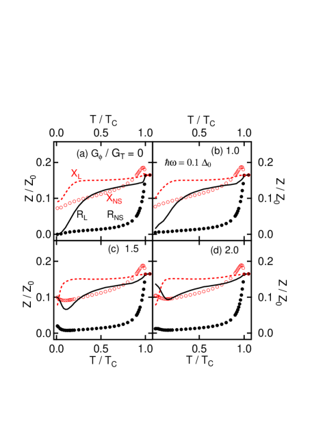
Figure 4: (color online). Impedance is plotted as a function of temperature for $R_{d}/R_{b}=0.2$ and $\hbar\omega=0.1\Delta_{0}$. The length of the normal metal is fixed at $L/\xi_{T_{C}}=1$. The symbols ($R_{\textrm{NS}}$ and $X_{\textrm{NS}}$) represent the results of impedance for the whole NS bilayer in Eq. (16). The lines ($R_{L}$ and $X_{L}$) are the local impedance at the surface of the normal metal given in Eq. (15).

Such anomalous behavior of impedance ($R_{L}>X_{L}$) is expected much wider temperature range when we consider stronger proximity effect. The results are shown in Figs. 5 and 6, where we choose $R_{d}/R_{b}=1$ in Fig. 5 and $R_{d}/R_{b}=5$ in Fig.6. The frequency of electromagnetic field remains unchanged from $\hbar\omega=0.1\Delta_{0}$ in both figures. At $G_{\phi}/G_{T}=1.5$, for instance, the crossover temperature is $T^{\ast}=0.02T_{C}$ for $R_{d}/R_{b}=0.2$ in Fig. 4(c), $T^{\ast}=0.17T_{C}$ for $R_{d}/R_{b}=1$ in Fig. 5(a), and $T^{\ast}=0.5T_{C}$ for $R_{d}/R_{b}=5$ in Fig. 6(a). In the same way at $G_{\phi}/G_{T}=2.0$, $T^{\ast}/T_{C}$ is 0.06, 0.3, and 0.8 for in Fig. 4(d), in Fig. 5(b), and in Fig. 6(b), respectively. Thus we conclude that the anomalous relation in the local impedance $R_{L}>X_{L}$ can be observed wider temperature range for larger $R_{d}/R_{b}$. On the other hand, the impedance of the whole NS bilayer always shows the usual relation $R_{\textrm{NS}}<X_{\textrm{NS}}$. The even-frequency Cooper pairs in the superconductor dominate the impedance of the bilayer. The nonmonotonic temperature dependence of $R_{\textrm{NS}}$ and $X_{\textrm{NS}}$, however, can be seen for $T<T^{\ast}$.

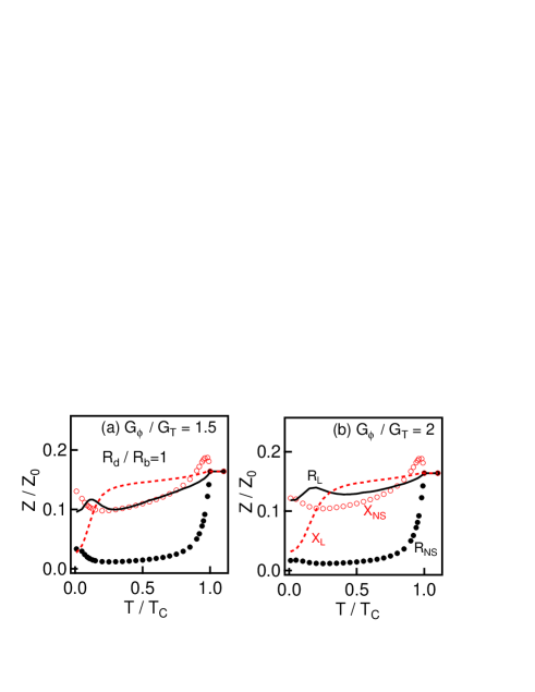
Figure 5: (color online). The results of impedance for $R_{d}/R_{b}=1$ and $\hbar\omega=0.1\Delta_{0}$.

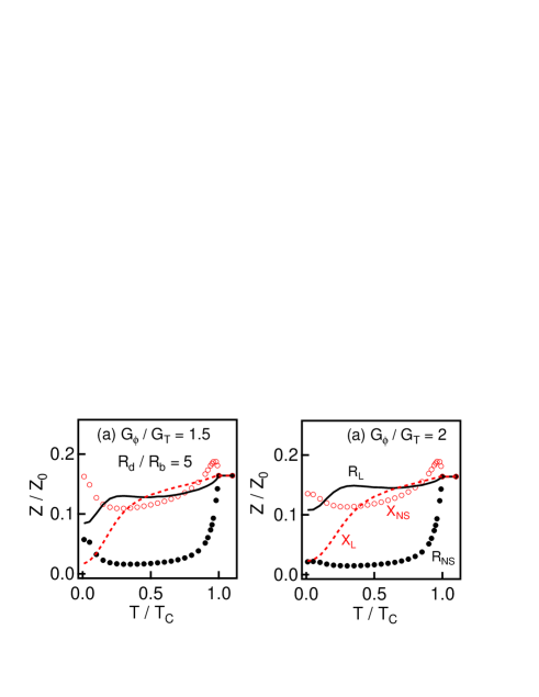
Figure 6: (color online). The results of impedance for $R_{d}/R_{b}=5$ and $\hbar\omega=0.1\Delta_{0}$.

Finally we look into the impedance for several choices of the frequency of electromagnetic field in Fig. 7, where we choose $G_{\phi}/G_{T}=1.5$ and $R_{d}/R_{b}=5$. The frequency of electromagnetic field is chosen as $\hbar\omega/\Delta_{0}=$ 0.01 and 0.5 in (a) and (b), respectively. Here we focus only on the local impedance $Z_{L}$. These results should be compared with Fig. 6(a) for $\hbar\omega/\Delta_{0}=$ 0.1. The crossover temperature to the anomalous relation is higher for smaller frequency. In Fig. 7(a), we find $T^{\ast}\sim 0.8T_{C}$. Thus it is easier to detect the anomalous relation $R>X$ in lower frequency in experiments. On the other hand, any sign for the odd-frequency pairs cannot be seen in the results for high frequency at $\hbar\omega=0.5\Delta_{0}$ in Fig. 7(b). Thus we need to tune the frequency of electromagnetic field to be much smaller than $\Delta_{0}/\hbar$.

On the basis of the calculated results, we predict that the anomalous relation of the impedance $R>X$ due to the odd-frequency Cooper pairs would be observed for high value of $G\phi/G_{T}$ and sufficiently low frequency of electromagnetic filed. The fabrication of NS bilayers using a thin ferromagnetic insulator blamire would realize large enough value of $G\phi/G_{T}$. It’s also important to note that, as shown in Ref. yoshizaki , in the case of thin ferromagnetic (F) film the effects of the exchange field and the $G\phi/G_{T}$ are equivalent. Therefore, the predicted anomalous behavior of impedance can be also realized in S/F junctions with thin F-layer. At the same time, the local impedance measurement is possible now machida . Thus the conclusion of this paper could be confirmed in experiments.

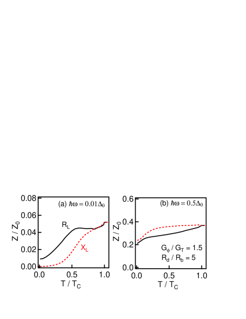
Figure 7: (color online). The results of local impedance for $R_{d}/R_{b}=5$ and $G_{\phi}/G_{T}=1.5$. We choose $\hbar\omega/\Delta_{0}=0.01$ in (a) and 0.5 in (b). These results should be compared with the results for $\hbar\omega/\Delta_{0}=0.1$ in Fig.6(a).

IV conclusion

We have studied the surface impedance ($Z=R-iX$) of a normal-metal-superconductor bilayers which has the spin-dependent potential at its junction interface. The complex conductivity is calculated from the quasiclassical Green function which is obtained by solving the Usadel equation numerically. The Effects of the spin-dependent potential at the interface is considered through the $G_{\phi}$-term in the Kupriyanov-Luckicev boundary condition at the junction interface. The spin-dependent potential produces the odd-frequency Cooper pairs in the normal metal. We conclude that the local impedance in the normal metal shows the unusual relationship $R>X$ when the odd-frequency Cooper pairs become dominant in the normal metal. The predicted results can be observed by recently developed local impedance measurement technique. In this paper, we consider spin-singlet $s$-wave superconductor as a bulk superconductor. It is a challenging issue to extend this calculation available for unconventional superconductor, spin-singlet $d$-wave d-wave , spin-triplet $p$-wave p-wave , and topological superconductors topological . In these systems, it is known that Andreev bound state or Majorana fermion governs charge transport Review .

V acknowledgement

This work was supported by KAKENHI(No. 22540355) and the ”Topological Quantum Phenomena” (No. 22103002) Grant-in Aid for Scientific Research on Innovative Areas from the Ministry of Education, Culture, Sports, Science and Technology (MEXT) of Japan.

References

- (1) V. L. Berezinskii, JETP Lett. 20, 287 (1974).
- (2) F. S. Bergeret, A. F. Volkov, and K. B. Efetov, Phys. Rev. Lett. 86, 4096 (2001); Rev. Mod. Phys. 77, 1321 (2005).
- (3) Y. Asano, Y. Tanaka, and A. A. Golubov, Phys. Rev. Lett. 98, 107002 (2007).
- (4) V. Braude and Yu. V. Nazarov, Phys. Rev. Lett. 98, 077003 (2007).
- (5) M. Eschrig and T. Löfwander, Nature Phys. 4, 138 (2008).
- (6) Ya. V. Fominov, A. F. Volkov, and K. B. Efetov, Phys. Rev. B75, 104509 (2007).
- (7) J. Linder, T. Yokoyama, and A. Sudbo, Phys. Rev. B 77, 174507 (2008); J. Linder, T. Yokoyama, Y. Tanaka, Y. Asano, and A. Sudbo, Phys. Rev. B 77, 174505 (2008); J. Linder, T. Yokoyama, A. Sudbø, and M. Eschrig, Phys. Rev. Lett. 102, 107008 (2009).
- (8) T. Yokoyama, Y. Tanaka, and A. A. Golubov, Phys. Rev. B 72, 052512 (2005), T. Yokoyama, Y. Tanaka, and A. A. Golubov, ibid 73, 094501 (2006).
- (9) T. Yokoyama, Y. Tanaka, and A. A. Golubov, Phys. Rev. B 75, 094514 (2007); Y. Sawa, T. Yokoyama, Y. Tanaka, and A. A. Golubov, ibid. 75, 134508 (2007).
- (10) K. Halterman, P. H. Barsic, and O. T. Valls, Phys. Rev. Lett. 99, 127002 (2007); P. H. Barsic and O. T. Valls, Phys. Rev.B 79, 014502 (2009).
- (11) M. Houzet and A. I. Buzdin, Phys. Rev. B 76, 060504(R) (2007).
- (12) R. S. Keizer, S. T. B. Goennenwein, T. M. Klapwijk, G. Miao, G. Xiao, and A. Gupta, Nature 439, 825 (2006).
- (13) M. S. Anwar, F. Czeschka, M. Hesselberth, M. Porcu, J. Aarts, Phys. Rev. B 82, 100501(R) (2010).
- (14) T. S. Khaire, M. A. Khasawneh, W. P. Pratt, Jr., and N. O. Birge, Phys. Rev. Lett. 104, 137002 (2010).
- (15) J. W. A. Robinson, J. D. S. Witt, and M. G. Blamire, Science 329, 59 (2010).
- (16) Y. Tanaka, A. A. Golubov, S. Kashiwaya, and M. Ueda, Phys. Rev. Lett. 99, 037005 (2007); Y. Tanaka, Y. Tanuma, A. A. Golubov, Phys. Rev. B 76, 054522 (2007).
- (17) Y. Tanaka and A. A. Golubov, Phys. Rev. Lett. 98, 037003 (2007).
- (18) Y. Tanaka and S. Kashiwaya, Phys. Rev. B 70, 012507 (2004); Y. Tanaka, S. Kashiwaya, and T. Yokoyama, ibid 71, 094513 (2005).
- (19) Y. Tanaka, Y. Asano, A. A. Golubov, and S. Kashiwaya, Phys. Rev. B 72, 140503(R) (2005).
- (20) Y. Asano, Y. Tanaka, and S. Kashiwaya, Phys. Rev. Lett. 96, 097007 (2006).
- (21) Y. Asano, Y. Tanaka, A. A. Golubov, and S. Kashiwaya, Phys. Rev. Lett. 99, 067005 (2007).
- (22) Ya. V. Fominov, JETP Lett. 86, 732 (2007).
- (23) Y. Asano, A. A. Golubov, Ya. V. Fominov, and Y. Tanaka, Phys. Rev. Lett. 107, 087001 (2011).
- (24) D. C. Mattis and J. Bardeen, Phys. Rev. 111, 412 (1958).
- (25) S. B. Nam, Phys. Rev. 156, 470 (1967).
- (26) A. A. Abrikosov, L. P. Gorkov, and I. E. Dzyaloshinski, Methods of Quantum Field Theory in Statistical Physics (Dover, New York, 1975). The negative pair density, discussed in the present paper, implies that the corresponding coefficient describing the response of the current to the vector potential, becomes negative in equations of the standard theory of superconductivity.
- (27) Y. Maeno, H. Hashimoto, K. Yoshida, S. Nishizaki, T. Fujita, J. G. Bednorz, and F. Lichtenberg, Nature 372, 532 (1994).
- (28) K. D. Usadel, Phys. Rev. Lett. 25, 507 (1970).
- (29) M. Yu. Kupriyanov and V. F. Lukichev, Sov. Phys. JETP 67, 1163 (1988).
- (30) D. Huertas-Hernando, Yu. V. Nazarov, and W. Belzig, Phys. Rev. Lett. 88, 047003 (2002).
- (31) A. Cottet, Phys. Rev. B 76, 224505 (2007).
- (32) D. Yoshizaki, A. A. Golubov, Y. Tanaka, and Y. Asano, Japanese Journ. Appl. Phys. 51, 010108 (2012)
- (33) K. Senapati, M. G. Blamire, and Z. H. Barber, Nature Materials 10, 849 (2011).
- (34) T. Yokoyama, Y. Tanaka, and N. Nagaosa, Phys. Rev. Lett. 106, 246601 (2011).
- (35) T. Machida, M. B. Gaifullin, S. Ooi, T. Kato, H. Sakata, and K. Hirata, Jpn. J. Appl. Phys. 49, 116701 (2010); T. Machida, M. B. Gaifullin, S. Ooi, T. Kato, H. Sakata, and K. Hirata, Applied Physics Express 2 025006 (2009).
- (36) Ya. V. Fominov, M. Houzet, and L. I. Glazman, Phys. Rev. B 84 224517 (2011).
- (37) K. Senapati, M. G. Blamire, and Z. H. Barber, Nature Materials 10, 849 (2011).
- (38) Y. Tanaka and S. Kashiwaya, Phys. Rev. Lett. 74, 3451 (1995); Y. Asano, Y. Tanaka, and S. Kashiwaya: Phys. Rev. B 69, 134501 (2004); Y. Tanaka, Y. V. Nazarov, and S. Kashiwaya: Phys. Rev. Lett. 90, 167003 (2003).
- (39) M. Yamashiro, Y. Tanaka, and S. Kashiwaya: Phys. Rev. B 56 7847 (1997); M. Yamashiro, Y. Tanaka, Y. Tanuma, and S. Kashiwaya: J. Phys. Soc. Jpn. 67, 3224 (1998); S. Kashiwaya, H. Kashiwaya, H. Kambara, T. Furuta, H. Yaguchi, Y. Tanaka, and Y. Maeno: Phys. Rev. Lett. 107 077003 (2011).
- (40) M. Sato and S. Fujimoto: Phys. Rev. B 79, 094504 (2009), Y. Tanaka, T. Yokoyama, A. V. Balatsky, and N. Nagaosa: Phys. Rev. B 79, 060505 (2009); J. D. Sau, R. M. Lutchyn, S. Tewari, and S. Sarma: Phys. Rev.Lett. 104, 040502 (2010); J. Alicea, Phys. Rev. B. 81, 125318 (2010).
- (41) S. Kashiwaya and Y. Tanaka, Rep. Prog. Phys. 63, 1641 (2000); Y. Tanaka, M. Sato and N. Nagaosa, J. Phys. Soc. Jpn. 81, 011013 (2012).