Photoemission time-delay measurements and calculations close to the 3s ionization minimum in Ar

Abstract

We present experimental measurements and theoretical calculations of photoionization time delays from the $3s$ and $3p$ shells in Ar in the photon energy range of 32-42 eV. The experimental measurements are performed by interferometry using attosecond pulse trains and the infrared laser used for their generation. The theoretical approach includes intershell correlation effects between the $3s$ and $3p$ shells within the framework of the random phase approximation with exchange (RPAE). The connection between single-photon ionization and the two-color two-photon ionization process used in the measurement is established using the recently developed asymptotic approximation for the complex transition amplitudes of laser-assisted photoionization. We compare and discuss the theoretical and experimental results especially in the region where strong intershell correlations in the $3s\to kp$ channel lead to an induced “Cooper” minimum in the 3s ionization cross-section.

I Introduction

Attosecond pulses created by harmonic generation in gases [1, 2] allow us to study fundamental light-matter interaction processes in the time domain. When an ultrashort light pulse impinges on an atom, a coherent ultra-broadband electron wave packet is created. If the frequency of the pulse is high enough, the electronic wave packet escapes by photoionization [3]. As in ultrafast optics, the group delay of an outgoing electron wave packet can be defined by the energy derivative of the phase of the complex photoionization matrix element. When photoionization can be reduced to one non-interacting angular channel ($L$), this phase is the same as the scattering phase $\eta_{L}$, which represents the difference between a free continuum wave and that propagating out of the effective atomic potential for the $L$-angular channel. In fact, the concept of time delay was already introduced by Wigner in 1955 to describe $s$-wave quantum scattering [4]. In collision physics, with both ingoing and outgoing waves the (Wigner) time delay is twice the derivative of the scattering phase.

In general, photoionization may involve several strongly interacting channels. Only in some special cases, the Wigner time delay can be conveniently used to characterize delay in photoemission. One such case might be valence shell photoionization of Ne in the 100 eV range [5, 6]. In this case, there is no considerable coupling between the $2s\to\epsilon p$ and $2p\to\epsilon s$ or $\epsilon d$ channels and $\epsilon d$ is strongly dominant over $\epsilon s$, following Fano’s propensity rule [7]. The case of valence shell photoionization of Ar in the 40 eV range [8] is more interesting. In this case, the $3s$ photoionization is radically modified by strong inter-shell correlation with $3p$ [9]. As a result, the $3s$ photoionization cross-section goes through a deep “Cooper” minimum at approximately 42 eV photon energy [10]. Such a feature is a signature of inter-shell correlation and cannot be theoretically described using any independent electron, e.g. Hartree-Fock (HF) model.

Recent experiments [5, 8] reported the first measurements of delays between photoemission from different subshells from rare gas atoms, thus raising considerable interest from the scientific community. Different methods for the measurements of time delays were proposed, depending on whether single attosecond pulses or attosecond pulse trains were used. The streaking technique consists in recording electron spectra following ionization of an atom by a single attosecond pulse in the presence of a relatively intense infrared (IR) pulse, as a function of the delay between the two pulses [11, 12]. Temporal information is obtained by comparing streaking traces from different subshells in an atom [5] or from the conduction and valence bands in a solid [13]. On the other hand, the so-called RABBIT (Reconstruction of attosecond bursts by ionization of two-photon transitions) method consists in recording photoelectron above-threshold-ionization (ATI) spectra following ionization of an atom by a train of attosecond pulses and a weak IR pulse, at different delays between the two fields [14]. Temporal information on photoionization is obtained by comparing RABBIT traces from different subshells in an atom [8]. The name of the technique, which we will use throughout, refers to its original use for the measurement of the group delay of attosecond pulses in a train [15].

Both methods involve absorption or stimulated emission of one or several IR photons, and it is important to understand the role of these additional transitions for a correct interpretation of the measured photoemission delays. A temporal delay difference of 21 as was measured for the photoionization from the $2s$ and $2p$ shells in neon using single attosecond pulses of 100 eV central energy [5]. Interestingly, the electron issued from $2p$ shell was found to be delayed compared to the more bound $2s$ electron. Similarly, delay differences on the order of $\sim 100$ as were measured for the photoionization from the $3s$ and $3p$ shells in argon using attosecond pulse trains with central energy around 35 eV. Again, the $3p$ electron appears to be delayed relative to the $3s$-electron, with a difference which depends on the excitation energy [8].

These experimental results stimulated several theoretical investigations, ranging from advanced photoionization calculations, including correlations effects [6], time-dependent numerical approaches [5, 16, 17, 18] to semi- analytical developments aiming at understanding the effect of the IR field on the measured time delays [19, 20, 21]. The picture which is emerging from this productive theoretical activity is that when the influence of the IR laser field is correctly accounted for, such time delay measurements may provide very interesting information on temporal aspects of many-electron dynamics.

The present work reports theoretical and experimental investigation of photoionization in the $3s$ and $3p$ shells in argon in the 32-42 eV photon energy range. Besides providing a more extensive description of the experimental and theoretical methods in [8], we improve the results in three different ways:

• We performed more precise measurements using a stabilized Mach- Zehnder interferometer [22] for the RABBIT method. The stabilization allows us to take scans during a longer time and thus to extract the phase more precisely. Some differences with the previous measurements are found and discussed.

• For the comparison with theory, we determined the phases of the single-photon ionization amplitudes using the Random Phase Approximation with Exchange (RPAE) method, which includes intershell correlation effects [9, 23, 24]. This represents a clear improvement to the calculations presented in [8], using Hartree-Fock data [25], especially in the region above 40 eV where photoionization of Ar passes through an interference minimum, owing to 3s-3p intershell correlation effects.

• Finally, we improved our calculation of the phase of a two-photon ionization process, thus making a better connection between the experimental measurements and the single photoionization calculated phases [20].

The paper is organized as follows. Section II presents the experimental setup and results. Section III describes the phase of one- and two-photon ionization processes using perturbation theory in an independent-electron approximation. Section IV includes inter-shell correlation using the RPAE method. A comparison between theory and experiment is presented in Section V.

II Experimental method and results

The experiments were performed with a Titanium:Sapphire femtosecond laser system delivering pulses of $30$ fs (FWHM) duration, centered at $800$ nm, with $1$ kHz repetition rate, and a pulse energy of $\sim$ 3 mJ. A beam splitter divides the laser output into the probe and the pump arm of a Mach-Zehnder interferometer (see Fig. 1). The energy of the probe pulses can be adjusted by a $\lambda/2$-plate followed by an ultra-thin polarizer. The pump arm is focused by a $\text{f}=50$ cm focusing mirror into a pulsed argon gas cell, synchronized with the laser repetition rate, in order to generate an attosecond pulse train via high-order harmonic generation. An aluminum filter of $200$ nm thickness blocks the fundamental radiation and subsequently a chromium filter of the same thickness selects photon energies of about $10$ eV bandwidth in the range of harmonics 21 to 27.

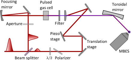
Figure 1: (color online) Schematic illustration of our experimental setup.

The probe and the pump arm of the interferometer are recombined on a curved holey mirror, transmitting the pump attosecond pulse train, but reflecting the outer portion of the IR probe beam. The exact position of the recombination mirror with respect to the focal position of the pump arm is essential in order to precisely match the wavefronts of the probe and XUV (extreme ultraviolet) beams. A toroidal mirror ($\text{f}=30$ cm) focuses both beams into the sensitive region of a magnetic bottle electron spectrometer (MBES), where a diffusive gas jet provides argon as detection gas. The relative timing between the ultrashort IR probe pulses and the attosecond pulse train can be reproducibly adjusted on a sub-cycle time scale due to an active stabilization of the pump-probe interferometer length [22].

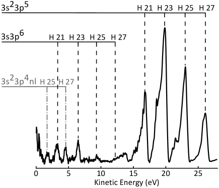
Figure 2: Electron spectrum obtained by ionizing Ar with four harmonics of orders 21, 23, 25 and 27. The ionization channels are shown on the top.

Figure  2 presents an electron spectrum obtained by ionizing Ar atoms with harmonics selected by both Al and Cr filters, with orders ranging from 21 to 27. We can clearly identify three ionization channels towards the $3s^{2}p^{5}$, $3s^{1}p^{6}$, and $3s^{2}3p^{4}n\ell$ ($n\ell=4p$ or $3d$) continua [26]. The corresponding ionization energies are 15.76, 29.2 and $\sim$ 37.2 eV. Note that the settings of the MBES were here chosen to optimize the spectral resolution at low energy. The large asymmetric profile obtained at high electron energy can be reduced by optimizing the MBES settings differently. The spectrum due to $3p$-ionization is strongly affected by the behavior of the ionization cross-section in this region. The relative intensities of the 21${}^{\textrm{st}}$ to the 27${}^{\textrm{th}}$ harmonics are approximately 0.2:0.7:1:1.

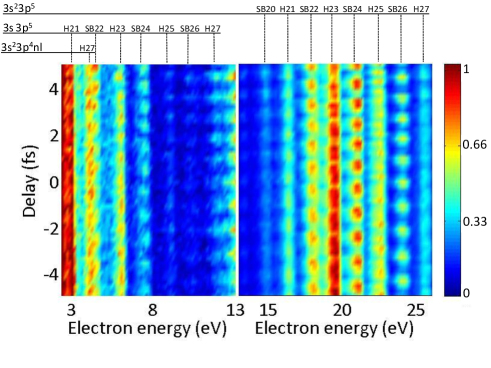
Figure 3: (color online) Electron spectrum as a function of time delay between the attosecond pulses and the IR laser. The signal strength is indicated by colors. The spectrum on the right ($3p$) follows that on the left ($3s$) with a factor of 6 reduction in the color code, and a slight overlap in energy.

Figure 3 shows a typical RABBIT spectrogram, i.e. electron spectra as a function of delay between pump and probe pulses. The electron yield is indicated as colors. Compared to the spectra obtained with the harmonics only, Fig. 3 includes electron peaks at sideband frequencies, including additional absorption or emission of one IR photon (see Fig. 4). The intensity of these sidebands oscillates with a delay at a frequency equal to $2\omega$, $\omega$ being the IR laser photon energy, according to

$$S_{2q}(\tau)=\alpha+\beta\cos(2\omega\tau-\Delta\phi_{2q}-\Delta\theta_{2q})$$ (1)

where $\alpha$ and $\beta$ are constant quantities, independent of the delay and $2q$ represents the total number of IR photons involved, i.e. an odd number to create harmonic $2q-1$ or $2q-1$ plus or minus one IR photon. $\Delta\phi_{2q}$ denotes the phase difference between two harmonics with order $2q+1$ and $2q-1$, while $\Delta\theta_{2q}$ arises from the difference in phase between the amplitudes of the two interfering quantum paths leading the same final state [Fig. 4 (a)]. $\tau_{A}=\Delta\phi_{2q}/2\omega$ can be interpreted as the group delay of the attosecond pulses [15]. We define in a similar way $\tau^{(2)}=\Delta\theta_{2q}/2\omega$ arising from the two-photon ionization process. Since the same harmonic comb is used for ionization in the $3s$ and $3p$ shells, the influence of the attosecond group delay can be subtracted and the delay difference $\tau^{(2)}(3s)-\tau^{(2)}(3p)$ can be deduced. The results of these measurements are indicated in Table 1 for sidebands 22, 24 and 26. We also indicate in the same table, previous results from [8]. It is quite difficult in such an experiment to estimate the uncertainty of our measurement. The stability of the interferometer is measured to be $\sim 50$ as. The relative uncertainty in comparing the phase offsets of different sideband oscillations is estimated to be of the same magnitude or even slightly better.

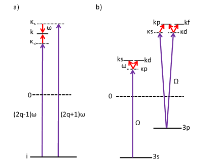
Figure 4: (color online) Energy level scheme of the processes discussed in the present work; (a) RABBIT principle; (b) Different channels in 2-photon ionization from the $3s$ and $3p$ subshells.

Table 1: Time delay measurements

Sideband	22	24	26
Photon energy (eV)	34.1	37.2	40.3
$\tau^{(2)}(3s)-\tau^{(2)}(3p)$
this work (as)	-80	-100	10
$\tau^{(2)}(3s)-\tau^{(2)}(3p)$,
[8] (as)	-40 (-90)	-110	-80
$\tau_{cc}(3s)-\tau_{cc}(3p)$ (as)	-150	-70	-40
$\tau^{(1)}(3s)-\tau^{(1)}(3p)$(as)	70	-30	50

Our measurements agree well with those of [8] for sideband 24. For sideband 22, the measurements performed in [8] could not resolve the sideband peak from electrons ionized by harmonic 27 towards the continuum $3s^{2}3p^{4}n\ell$ (see Fig. 3). A new analysis done by considering only the high energy part of the sideband peak leads to the number indicated in parenthesis in the table, which is in good agreement with the present measurement. There is, however, a difference for the delay measured at sideband 26. We will comment on this difference in Section V.

III Theory of one and two-photon ionization

To interpret the results presented above, we relate the one-photon ionization delays to the delays measured in the experiment. Using lowest-order perturbation theory, the transition matrix elements in one and two-photon ionization are

$$M^{(1)}(\vec{k}) = -iE_{\Omega}\langle\vec{k}|z|i\rangle,$$ (2)

$$M^{(2)}(\vec{k}) = -iE_{\omega}E_{\Omega}\lim_{\varepsilon\to 0^{+}}\int\!\!\!\!\!\!\!\!\sum_{\nu}{\frac{\langle\vec{k}|z|\nu\rangle\langle\nu|z|i\rangle}{\epsilon_{i}+\Omega-\epsilon_{\nu}+i\varepsilon}}.$$ (3)

Atomic units are used throughout. We choose the quantization axis ($z$) to be the (common) polarization vector of the two fields. The complex amplitudes of the laser and harmonic fields are denoted by $E_{\omega}$ and $E_{\Omega}$, with photon energies $\omega$ and $\Omega$, respectively. The initial state is denoted $|i\rangle$ and the final state $|\vec{k}\rangle$. The energies of the initial and intermediate states are denoted $\epsilon_{i}$ and $\epsilon_{\nu}$, respectively. The sum in $M^{(2)}$ is performed over all possible intermediate states $|\nu\rangle$ in the discrete and continuum spectrum. The infinitesimal quantity $\varepsilon$ is added to ensure the correct boundary condition for the ionization process, so that the matrix element involves an outgoing photoelectron. The magnitude of the final momentum is restricted by energy conservation to $\epsilon=k^{2}/2=\Omega+\epsilon_{i}$ for one photon and $\epsilon=k^{2}/2=\Omega+\omega+\epsilon_{i}$ for two-photon absorption. The two-photon transition matrix element involving emission of a laser photon can be written in the same way, with $\omega$ replaced by $-\omega$ in the energy conservation relation and $E_{\omega}$ replaced by its conjugate.

The next step consists in separating the angular and radial parts of the wavefunctions. The different angular channels involved are indicated in Fig. 4(b). We split the radial and angular dependence in the initial state as $\langle{\bm{r}}|i\rangle=Y_{l_{i}m_{i}}(\hat{r})R_{n_{i}l_{i}}(r)$ and use the partial wave expansion in the final state

$$\langle{\bm{r}}|\vec{k}\rangle=(8\pi)^{\frac{3}{2}}\displaystyle\sum_{L,M}i^{L}e^{-i\eta_{L}(k)}Y^{*}_{LM}(\hat{k})Y_{LM}(\hat{r})R_{kL}(r).$$ (4)

We perform the spherical integration in Eq. (1) and obtain

$$M^{(1)}(\vec{k})\propto\sum_{L=l_{i}\pm 1\atop M=m_{i}}e^{i\eta_{L}(k)}i^{-L}Y_{LM}(\hat{k})$$

$$\left(\begin{array}[]{rrr}L&1&l_{i}\\ -M&0&m_{i}\\ \end{array}\right)\!T^{(1)}_{L}(k),$$ (7)

where the reduced dipole matrix element is defined as

$$T^{(1)}_{L}(k)=\hat{L}\hat{l}_{i}\left(\begin{array}[]{rrr}L&1&l_{i}\\ 0&0&0\\ \end{array}\right)\\ \langle R_{kL}|r|R_{n_{i}l_{i}}\rangle$$ (8)

using $3j$-symbols and with the notation $\hat{l}=\sqrt{2l+1}$. The reduced matrix element (8) is real. When the dipole transition with the increased momentum $L=l_{i}+1$ is dominant, which is often the case [7], the phase of the complex dipole matrix element $M^{(1)}$ is simply equal to

$$\arg[M^{(1)}(k)]=\eta_{L}(k)-L\pi/2.$$ (9)

(There is also a contribution from the fundamental field which we do not write here, as well as trivial phases, e.g from the spherical harmonic when $M\neq 0$ [20]). Similarly, for two-photon ionization,

$$M^{(2)}(\vec{k})\propto\sum_{L=\lambda\pm 1,\lambda=l_{i}\pm 1\atop M=\mu=m_{i}}e^{i\eta_{L}(k)}i^{-L}Y_{LM}(\hat{k})\,$$ (10)

$$\left(\begin{array}[]{rrr}L&1&\lambda\\ -M&0&\mu\\ \end{array}\right)\left(\begin{array}[]{rrr}\lambda&1&l_{i}\\ -\mu&0&m_{i}\\ \end{array}\right)T^{(2)}_{L\lambda}(k).$$ (15)

where

$$T^{(2)}_{L\lambda}(k)=\hat{L}\hat{\lambda}^{2}\hat{l}_{i}\left(\begin{array}[]{rrr}L&1&\lambda\\ 0&0&0\\ \end{array}\right)\\ \left(\begin{array}[]{rrr}\lambda&1&l_{i}\\ 0&0&0\\ \end{array}\right)\\ \langle R_{kL}|r|\rho_{\kappa\lambda}\rangle.$$ (16)

Here, we have introduced the radial component of the perturbed wave function,

$$|\rho_{\kappa\lambda}\rangle=\lim_{\varepsilon\to 0^{+}}\int\!\!\!\!\!\!\!\!\sum_{\nu}\frac{|R_{\nu\lambda}\rangle\langle R_{\nu\lambda}|r|R_{n_{i}l_{i}}\rangle}{\epsilon_{i}+\Omega-\epsilon_{\nu}+i\varepsilon}.$$ (17)

where the sum is performed over the discrete and continuum spectrum. $\kappa$ denotes the momentum corresponding to absorption of one harmonic photon such that the energy denominator goes to zero ($\kappa^{2}/2=\epsilon_{i}+\Omega$). The summation can be decomposed into three terms, the discrete sum over states with negative energy, a Cauchy principal part integral where the pole has been removed (both these terms are real) and a resonant term which is purely imaginary. The important conclusion is that in contrast to the radial one-photon matrix element, the radial two-photon matrix element is a complex quantity.

To evaluate the phase of this quantity, as explained in more details in [20], we approximate $R_{kL}(r)$ and $\rho_{\kappa\lambda}(r)$ by their asymptotic values. We have, for example,

$$\rho_{\kappa\lambda}(r) \approx-\sqrt{\frac{2}{\pi\kappa}}\langle R_{\kappa\lambda}|r|R_{n_{i}l_{i}}\rangle$$ (18)

$$\!\!\!\frac{1}{r}\exp\left\{i\left[\kappa r+\frac{\ln(2\kappa r)}{\kappa}+\eta_{\lambda}(\kappa)-\frac{\pi\lambda}{2}\right]\right\}.$$

This allows us to evaluate analytically the integral $\langle R_{kL}|r|\rho_{\kappa\lambda}\rangle$ in Eq. (16). We obtain

$$\arg\left[T^{(2)}_{L\lambda}(k)\right] \approx(L-\lambda)\frac{\pi}{2}$$ (19)

$$+\eta_{\lambda}(\kappa)-\eta_{L}(k)+\phi_{cc}(k,\kappa),$$

where $\phi_{cc}(k,\kappa)$ is the phase associated to a continuum-continuum radiative transition resulting from the absorption of IR photons in the presence of the Coulomb potential. It is independent from the characteristics of the initial atomic state, in particular its angular momentum. An important consequence is that, when inserting the asymptotic form Eq. (18) in Eq. (10), the scattering phase $\eta_{L}$ is canceled out, so that the total phase will not depend on the angular momentum of the final state. In the case of a dominant intermediate channel $\lambda$, the phase of the complex two-photon matrix element $M^{(2)}(k)$ is equal to

$$\arg[M^{(2)}(k)]=\eta_{\lambda}(\kappa)-\lambda\pi/2+\phi_{cc}(k,\kappa).$$ (20)

It is equal to the one-photon ionization phase towards the intermediate state with momentum $\kappa$ and angular momentum $\lambda$ plus the additional “continuum-continuum” phase. The difference of phase which is measured in the experiment is therefore given by

$$\Delta\theta_{2q}=\eta_{\lambda}(\kappa_{>})-\eta_{\lambda}(\kappa_{<})~{}+~{}\phi_{cc}(k,\kappa_{>})-\phi_{cc}(k,\kappa_{<}).$$ (21)

where $\kappa_{>}$, $\kappa_{<}$ are the momenta corresponding to the highest (lowest) continuum state in Fig. 4(a). Dividing this formula by $2\omega$, we have

$$\tau^{(2)}(k)=\tau^{(1)}(k)+\tau_{cc}(k),$$ (22)

where

$$\tau^{(1)}(k)=\frac{\eta_{\lambda}(\kappa_{>})-\eta_{\lambda}(\kappa_{<})}{2\omega},$$ (23)

is a finite difference approximation to the Wigner time delay $d\eta_{\lambda}/d\epsilon$ and thus reflects the properties of the electronic wave packet ionized by one-photon absorption into the angular channel $\lambda$. $\tau^{(2)}$ also includes a contribution from the IR field which is independent of the angular momentum,

$$\tau_{cc}(k)=\frac{\phi_{cc}(k,\kappa_{>})-\phi_{cc}(k,\kappa_{<})}{2\omega}.$$ (24)

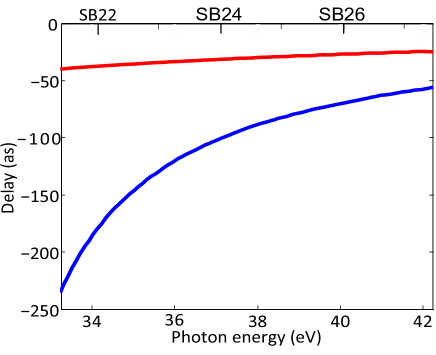
Figure 5: (color online) Continuum-continuum delay $\tau_{cc}$ as a function of excitation photon energy for the two subshells $3s$ (red) and $3p$ (blue) for an IR photon energy of 1.55 eV (800 nm wavelength).

We refer the reader to [20] for details about how to calculate $\tau_{cc}$. Fig. 5 shows $\tau_{cc}$ as a function of photon energy, for the two subshells $3s$ and $3p$ and for the IR photon energy $\omega=1.55$ eV used in the experiment. The corresponding difference in delays for the $3s$ and $3p$ subshells is only due to the difference in ionization in energy between the two shells (13.5 eV). We also indicate in Table I the measurement-induced delays for the three considered sidebands.

The processes discussed in this section can be represented graphically by Feynman-Goldstone diagrams displayed Fig. 6(a,b). The straight lines with arrows represent electron (arrow pointing up) or hole (arrow pointing down) states, respectively. The violet and red wavy lines represent interaction with the XUV and IR fields. We are neglecting here two-photon processes where the IR photon is absorbed first [20].

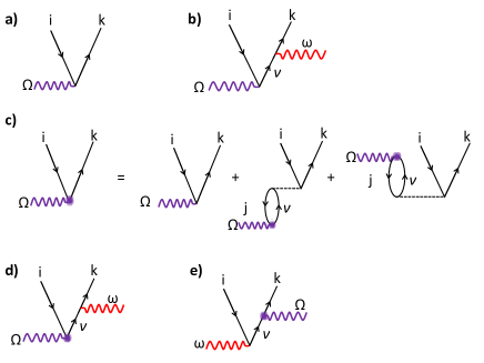
Figure 6: (color online) Feynman-Goldstone diagrams representing one-photon (a) and two-photon (b) ionization processes. (c) Diagrammatic representation of the RPAE equations. The second and third diagrams on the right hand side refer to time-forward and time-reversed respectively. (d) Two-photon ionization including intershell correlation effects. (e) Two-photon ionization with the XUV photon absorbed after the IR photon.

IV Intershell correlation effects

To include inter-shell correlation effects, we use the random phase approximation with exchange (RPAE) [9]. In this approximation, the dipole matrix element of single photoionization is replaced by a “screened” matrix element $\langle k|Z|i\rangle$, which accounts for correlation effects between the $3s$ and $3p$ subshells. These screened matrix elements, represented graphically in Fig. 6(c), are defined by the self-consistent equation:

$$\langle\vec{k}|Z|i\rangle = \langle\vec{k}|z|i\rangle+\lim_{\varepsilon\to 0^{+}}\int\!\!\!\!\!\!\!\!\sum_{\nu}\Bigg{[}\frac{\langle\nu|Z|j\rangle\langle j\vec{k}|V|\nu i\rangle}{\Omega-\epsilon_{\nu}+\epsilon_{j}+i\varepsilon}$$ (25)

$$\hskip 21.33955pt-\frac{\langle j|Z|\nu\rangle\langle\nu\vec{k}|V|ji\rangle}{\Omega+\epsilon_{\nu}-\epsilon_{j}}\Bigg{]},$$

where $i$ and $j$ are $3s$ or $3p$ or vice versa and $V=1/r_{12}$ is the Coulomb interaction. The sum is performed over the discrete as well as continuum spectrum. The Coulomb interaction matrices $\langle j\vec{k}|V|\nu i\rangle$ and $\langle\nu\vec{k}|V|ij\rangle$, represented by dashed lines in Fig. 6(c), describe the so-called time-forward and time-reversed correlation processes (Note that the time goes upwards in the diagrams). If we replace $Z$ by $z$ in the right term in Eq. (25), we obtain a perturbative expansion to the first order in the Coulomb interaction. More generally, the use of the self-consistent screened matrix elements [Eq.(25)] implies infinite partial sums over two important classes of so-called “bubble” diagrams. Each bubble consists of an electron-hole pair $\nu j$, which interacts via $1/r_{12}$ with final electron-hole pair $\vec{k}i$. The energy integration in the time-forward term of Eq. (25) (first line) contains a pole and the screened matrix element acquires an imaginary part and therefore an extra phase. For a single dominant channel $L$, the phase of the one-photon matrix element [see Eq.(9)] becomes:

$$\arg[M^{(1)}(k)]=\eta_{L}(k)+\delta_{L}(k)-L\pi/2,$$ (26)

where $\delta_{L}(k)=\delta_{i\to kL}$ denotes the additional phase due to the correlations accounted within the RPAE. The photoemission time delay is then determined by the sum of two terms:

$$\tau^{(1)}=\frac{d\eta_{L}}{d\epsilon}+\frac{d\delta_{L}}{d\epsilon}.$$ (27)

The first term represents the time delay in the independent electron approximation, equal to the derivative of the photoelectron scattering phase in the combined field of the nucleus and the remaining atomic electrons. The second term is the RPAE correction due to inter-shell correlation effects.

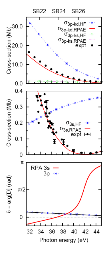
Figure 7: (color online) Top panel: The photoionization cross-sections $\sigma_{3p\to kd}$ calculated in the HF (blue dotted line) and RPAE (red solid line) approximations, are compared with the $\sigma_{3p\to ks}$ cross-sections (HF, green open circles, RPAE, purple dashed line). The experimental data for the $\sigma_{3p}$ cross-section are from Ref. [30]. Middle panel: Photoionization cross-sections $\sigma_{3s}$ calculated in the HF (blue dotted line) and RPAE(red solid line) approximations, are compared with experimental data [10]. Bottom panel: Correlation-induced phase shifts for the $3s$ and $3p$ dipole matrix elements.

We solve the system of integral equations (25) numerically using the computer code developed by Amusia and collaborators [27]. The basis of occupied atomic states (holes) $3s$ and $3p$ is defined by the self-consistent HF method [28]. The excited electron states are calculated within the frozen-core HF approximation [29]. We present some results for one-photon ionization in Fig. 7. On the top panel, we show the partial photoionization cross-sections from the $3p$-state calculated using the HF and RPAE approximations (see figure caption). From this plot, we see that the $3p\to kd$ transition is clearly dominant at low photon energies. Intershell correlation effects are more important for the $3p\to ks$ than for the $3p\to kd$ transition. The sum of the two partial cross sections calculated with the RPAE correction (red and green lines) is very close to the the experimental data (solid circles) [30]. The middle panel presents the calculated cross-section for $3s$-ionization and compares it to the experimental data from [10]. The RPAE correction is here essential to reproduce the behavior of the cross-section which, in this spectral region, is a rapid decreasing function of photon energy.

The bottom panel shows the correlation-induced phase shifts $\delta_{3s\to kp}$ and $\delta_{3p\to kd}$ from the same RPAE calculation. We observe that the RPAE phase correction $\delta_{3p\to kd}$ is relatively weak. In contrast, $\delta_{3s\to kp}$ varies significantly with energy, especially near the “Cooper” minimum. This qualitative difference can be explained by a different nature of the correlations in the $3p$ and $3s$ shells. In the $3p$ case, the correlation takes place mainly between the electrons that belong to the same shell with not much influence of the inter-shell correlation with $3s$. We confirmed this conclusion by performing a separate set of RPAE calculations with only the $3p$ shell included. These calculations lead to essentially the same results for $3p$ ionization as the complete calculations. In the case of intrashell correlation, the time-forward process [see Fig. 6(c)] is effectively accounted for by calculating the photoelectron wave function in the field of a singly charged ion. It is therefore excluded from Eq. (25) to avoid double count. The remaining time-reversed term [second line in Eq. (25)] does not contain any poles and therefore does not contribute to an additional phase to the corresponding dipole matrix element. The small phase $\delta_{3p\to kd}$ is due to intershell correlation which is indeed weak. In contrast, $3s$-ionization is strongly affected by correlation with the $3p$ shell. Consequently, the RPAE phase correction $\delta_{3s\to kp}$, which comes from the correlation with the $3p$ shell in the time-forward process, is large and exhibits a rapid variation with energy (a $\pi$ phase change) in the region where the cross section decreases significantly.

Finally, we generalize our theoretical derivation of two-photon ionization to including the effect of inter-shell correlation on the XUV photon absorption. As shown graphically in the diagram in Fig. 6 (d), we replace the (real) transition matrix element corresponding to one-XUV photon absorption by a (complex) screened matrix element, with an additional phase term. As a consequence the phase of the two-photon matrix element becomes:

$$\arg[M^{(2)}(k)]=\eta_{\lambda}(\kappa)+\delta_{\lambda}(\kappa)-\lambda\pi/2+\phi_{cc}(k,\kappa).$$ (28)

The time delay measured in the experiment is expressed as before as $\tau^{(2)}(k)=\tau^{(1)}(k)+\tau_{cc}(k)$, with $\tau^{(1)}(k)$ modified by intershell correlation:

$$\tau^{(1)}(k)=\frac{\eta_{\lambda}(\kappa_{+})-\eta_{\lambda}(\kappa_{-})}{2\omega}+\frac{\delta_{\lambda}(\kappa_{+})-\delta_{\lambda}(\kappa_{-})}{2\omega}.$$ (29)

Figure 8 presents calculated time delays $\tau^{(1)}$ for $3s\to kp$, $3p\to ks$ and $3p\to kd$ channels. The ionization delays from the $3p$ channel do not vary much with photon energy and remain small. The $3p\to ks$ delay is negligible while it takes about 70 as more time for the wave packet to escape towards the $d$ channel, due to the angular momentum barrier. The wave packet emitted from the $3s$ channel takes considerably more time to escape, especially in the region above 40 eV, owing to strong intershell correlation leading to screening by the $3p$ electrons.

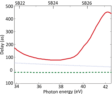
Figure 8: (color online) Ionization delay for the three angular channels $3p\to kd$ (blue dashed), $3p\to ks$ (green dashed) and $3s\to kp$ (red solid line).

V Comparison between theory and experiment

We present in Fig. 9 a comparison between our experimental results (see Table 1) and our calculations. The dashed blue and solid red lines refer to the independent-electron HF and RPAE calculations, respectively. The circles refer to the results of [8], while the other symbols (with error bars both in central energy and delay) are the results obtained in the present work. Regarding the two sets of experimental results, they agree very well, except for that obtained at the highest energy corresponding to the sideband 26. Our interpretation is that we may be approaching the rapidly varying feature due to $3s-3p$ intershell correlation, leading to a large dispersion of the possible time delays (Note, however, that its position seems to be shifted compared to the RPAE result). The experimental and RPAE results agree well for the first sideband but less for the two higher energy sidebands. Surprisingly and perhaps accidentally the HF calculation gives there a closer agreement with the experiment.

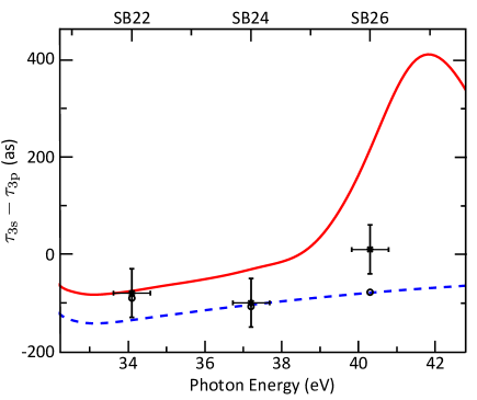
Figure 9: (color online) Comparison between our theoretical calculations (dashed blue line, HF, red line, RPAE) and experiments (circles [8], crosses, present work)

We now discuss possible reasons for the discrepancy. Our calculation of the influence of the dressing by the IR laser field is approximate. It only uses the asymptotic form of the continuum wave functions (both in the final and intermediate states), thereby neglecting the effect of the core. This approximation should be tested against theoretical calculations, and especially in a region where correlation effects are important. We also neglect the influence of the two-photon processes where the IR photon is absorbed (or emitted) first [31] [see Fig. 6 (e)]. The corresponding matrix elements are usually small, except possibly close to a minimum of the cross section, where the other process, usually dominant, is strongly reduced. Interestingly, in such a scenario, the IR radiation would not simply be a probe used for the measurement of the phase of a one-photon process, but would modify (control) the dynamics of the photoemission on an attosecond time scale. Finally, in our theoretical calculation, correlation effects are only accounted for in the single ionization process (XUV absorption). Additional correlation effects surrounding the probing, e.g. after the IR photon is absorbed might play a role.

In conclusion, the results shown above point out to the need for explicit time-dependent calculations, which would account for many-electron correlation and include not only one-photon but also two-photon ionization. We also plan to repeat these experimental measurements using attosecond pulses with a large and tunable bandwidth. Our results demonstrate the potential of the experimental tools using single attosecond pulses [5] or attosecond pulse trains [8]. These tools now enable one to measure atomic and molecular transitions, more specifically, quantum phases and phase variation, i.e. group delays, which could not be measured previously.

Acknowledgements

We thank G. Wendin for useful comments. This research was supported by the Marie Curie program ATTOFEL (ITN), the European Research Council (ALMA), the Joint Research Programme ALADIN of Laserlab-Europe II, the Swedish Foundation for Strategic Research, the Swedish Research Council, the Knut and Alice Wallenberg Foundation, the French ANR-09-BLAN-0031-01 ATTO-WAVE program, COST Action CM0702 (CUSPFEL).

References

- [1] P. B. Corkum and F. Krausz, Nat. Phys.3, 381 (2007).
- [2] F. Krausz and M. Ivanov, Rev. Mod. Phys. 81, 163 (2009).
- [3] V. Schmidt, Rep. Prog. Phys. 55, 1483 (1992).
- [4] E. P. Wigner, Phys. Rev. 98, 145 (1955).
- [5] M. Schultze et al., Science 328, 1658 (2010).
- [6] A.S. Kheifets and I.A. Ivanov, Phys. Rev. Lett. 105, 233002 (2010).
- [7] U. Fano, Phys. Rev. A 32, 617 (1985).
- [8] K.Klünder et al., Phys. Rev. Lett. 106, 143002 (2011).
- [9] M. Y. Amusia et al., Phys. Lett. A 40, 361 (1972).
- [10] B. Möbus et al., Phys. Rev. A 47, 3888 (1993).
- [11] E. Goulielmakis et al., Science 305, 1267 (2004).
- [12] G. Sansone et al., Science 314, 443 (2006).
- [13] Cavalieri, A. et al., Nature 449, 1029 (2007).
- [14] P. M. Paul et al., Science 292, 1689 (2001).
- [15] Y. Mairesse et al., Science 302, 1540 (2003).
- [16] V.S. Yakovlev, J. Gagnon, N. Karpowicz and F. Krausz, Phys. Rev. Lett. 105, 073001 (2010).
- [17] S. Nagele, R. Pazourek, J. Feist and J. Burgdorfer, J. Phys. B: Atom. Molec. Opt. Phys. 44, 081001 (2011); Phys. Rev. A 85, 033401 (2012).
- [18] L. R. Moore, M. A. Lysaght,J. S. Parker, H. W. vanderHart and K. T. Taylor, Phys. Rev. A 84, 061404 (2011).
- [19] C.-H. Zhang and U. Thumm, Phys. Rev. A 84, 033401 (2011).
-
[20]
J. M. Dahlstrom et al., J. Chem. Phys., in press (2012).
http://dx.doi.org/10.1016/j.chemphys.2012.01.017 - [21] M. Ivanov and O. Smirnova, Phys. Rev. Lett. 107, 213605 (2011).
- [22] D. Kroon et al., in preparation.
- [23] G. Wendin, J. Phys. B: Atom. Molec. Opt. Phys. 5, 110 (1972).
- [24] A. L’Huillier, L. Jönsson and G. Wendin, Phys. Rev. A 33, 3938 (1986).
- [25] D.J. Kennedy and S.T. Manson, Phys. Rev. A 5, 227 (1972).
- [26] A.Kikas et al., J. Electron Spectrosc. Rel. Phenom. 77 241, (1996).
- [27] M. Ia. Amusia and L. V. Chernysheva, Computation of atomic processes : A handbook for the ATOM programs. Institute of Physics Pub., Bristol, UK, 1997.
- [28] L. V. Chernysheva, N. A. Cherepkov, and V. Radojevic, Comp. Phys. Comm. 11, 57 (1976).
- [29] L. V. Chernysheva, N. A. Cherepkov, and V. Radojevic, Comp. Phys. Comm. 18, 87 (1979).
- [30] J.A.R. Samson and W.C. Stolte, J. Electron Spectrosc. Rel. Phenom. 123, 265 (2002).
- [31] V. Véniard, R. Taïeb, and A. Maquet, Phys. Rev. A 54, 721 (1996).