The Dynamics of Influence Systems

Abstract

Influence systems form a large class of multiagent systems designed to model how influence, broadly defined, spreads across a dynamic network. We build a general analytical framework which we then use to prove that, while sometimes chaotic, influence dynamics of the diffusive kind is almost always asymptotically periodic. Besides resolving the dynamics of a popular family of multiagent systems, the other contribution of this work is to introduce a new type of renormalization-based bifurcation analysis for multiagent systems.

1 Introduction

The contribution of this paper is twofold: (i) to formulate an “algorithmic calculus” for continuous, discrete-time multiagent systems; and (ii) to resolve the behavior of a popular type of social dynamics that had long resisted analysis. In the process, we also introduce a new approach to time-varying Markov chains. Diffusive influence systems are piecewise-linear dynamical systems ${\mathbf{x}}\mapsto P({\mathbf{x}}){\mathbf{x}}$, which are specified by a piecewise-constant function $P$ mapping any ${\mathbf{x}}\in{\mathbb{R}}^{n}$ to an $n$-by-$n$ stochastic matrix $P({\mathbf{x}})$. We prove that, while sometimes chaotic, such systems are almost surely attracted to a fixed point or a limit cycle.

As in statistical mechanics, the difficulty of analyzing influence systems comes from the tension between two opposing forces: one, caused by the map’s discontinuities, is “entropic” and leads to chaos; the other one, related to the Lyapunov exponents, is “energetic” and pulls the system toward an attracting manifold within which the dynamics is periodic. The challenge is to show that, outside a vanishingly small critical region in parameter space, entropy always loses. Because the interaction topology changes all the time (endogenously), the proof relies heavily on an algorithmic framework to monitor the flow of information across the system. As a result, this work is, at its core, an algorithmic study in dynamic networks. Influence systems include finite Markov chains as a special case but the differences are deep and far-reaching: whereas Markov chains have predictable dynamics, influence systems can be chaotic even for small $n$; whereas the convergence of a Markov chain can be checked in polynomial time, the convergence of an influence system is undecidable. Our main result is that this bewildering complexity is in fact confined to a vanishing region of parameter space. Typically, influence systems are asymptotically periodic.

Influence and social dynamics.

There is a context to this work and this is where we begin. An overarching ambition of social dynamics is to understand and predict the collective behavior of agents influencing one another across an endogenously changing network [14]. HK systems have emerged in the last decade as a prototypical platform for such investigations [6, 7, 27, 28, 32, 34, 35, 37, 38, 40]. To unify its varied strands (eg, bounded-confidence, bounded-influence, truth-seeking, Friedkin-Johnsen type, deliberative exchange) into a single framework and supply closed-loop analogs to standard consensus models [5, 36, 41], we introduce influence systems. These are discrete-time dynamical systems ${\mathbf{x}}\mapsto f({\mathbf{x}})$ in $({\mathbb{R}}^{d})^{n}$: each “coordinate” $x_{i}$ of the state ${\mathbf{x}}=(x_{1},\ldots,x_{n})$ is a $d$-tuple encoding the location of agent $i$ as a point in ${\mathbb{R}}^{d}$; with any state ${\mathbf{x}}$ is associated a directed graph ${\mathcal{G}}({\mathbf{x}})$ with the $n$ agents as nodes. Each coordinate function $f_{i}$ of the map $f=(f_{1},\ldots,f_{n})$ takes as input the neighbors of agent $i$ in ${\mathcal{G}}({\mathbf{x}})$ and outputs the new location $f_{i}({\mathbf{x}})$ of agent $i$ in $d$-space. One should think of agent $i$ as a “computer” and $x_{i}$ as its “memory.” All influence systems in this work will be assumed to be diffusive, meaning that at each step an agent may move only within the convex hull of its neighbors. Note that the system ${\mathbf{x}}\mapsto P({\mathbf{x}}){\mathbf{x}}$ in the opening paragraph corresponds to the one-dimensional case.

Influence systems arise in processes as diverse as chemotaxis, synchronization, opinion dynamics, flocking, swarming, and rational social learning. Typically, a natural algorithm directs $n$ autonomous agents to obey two sets of rules: (i) one of them determines, on the basis of the system’s current state ${\mathbf{x}}$, which agent communicates with which one; (ii) the other one specifies how an agent updates its state by processing the information it receives from its neighbors. Diffusive influence systems are central to social dynamics insofar as they extend the fundamental concept of diffusion to autonomous agents operating within dynamic, heterogeneous environments. This stands in sharp contrast with the classic brand of diffusion found in physics and chemistry, which assumes passive particles subject to identical laws. Naturally, influence systems are “downward-compatible” and can model standard (discrete) diffusion as well. They also allow exogeneities (eg, diffusion-reaction) via the addition of special-purpose agents. Autonomy and heterogeneity are the defining features of influence systems: they grant agents the freedom to have their own, distinct decision procedures to choose their neighbors as they please and act on the information collected from them. This explains their ubiquity among natural algorithms.

The model.

In a diffusive influence system, $f({\mathbf{x}})=(P({\mathbf{x}})\otimes\text{Id})\,{\mathbf{x}}$, where $P({\mathbf{x}})$ is a stochastic matrix whose positive entries correspond to the edges of ${\mathcal{G}}({\mathbf{x}})$ and are rationals larger than some arbitrarily small $\rho>0$. We form the Kronecker product with the $d$-by-$d$ identity matrix to perform the averaging along each coordinate axis. We grant the agents a measure of self-confidence by adding a self-loop to each node of ${\mathcal{G}}({\mathbf{x}})$. Agent $i$ computes the $i$-th row of $P({\mathbf{x}})$ by means of its own algebraic decision tree; that is, on the basis of the signs of a finite number of $dn$-variate polynomials evaluated at the coordinates of ${\mathbf{x}}$. This high level of generality allows ${\mathcal{G}}({\mathbf{x}})$ to be specified by any first-order sentence over the reals: In a recent bird flocking model [4], for instance, the communication graph joins every agent to its 7 nearest neighbors. We show below how to reduce the dimension to $d=1$ and linearize the system so that $P({\mathbf{x}})=P_{c}$, for any ${\mathbf{x}}\in c$, where $c$ is any atom (open $n$-cell) of an arrangement of hyperplanes in ${\mathbb{R}}^{n}$, called the switching partition (SP ). An influence system is called bidirectional if ${\mathcal{G}}_{ij}\equiv{\mathcal{G}}_{ji}$ (with ${\mathcal{G}}=({\mathcal{G}}_{ij})$), which implies that ${\mathcal{G}}({\mathbf{x}})$ is undirected. Such a system is further called metrical if ${\mathcal{G}}_{ij}$ is solely a function of $|x_{i}-x_{j}|$. Homogeneous HK systems [27, 28, 32] constitute the canonical example of a metrical system. We assume that all the relevant parameters (matrix entries, number and coefficients of hyperplanes, $\rho$, etc) can be encoded as rationals over $O(\log n)$ bits: this assumption can be freely relaxed—in fact, the bit lengths can be arbitrarily large as a function of $n$—and is only made to simplify the notation.

Past work and present contribution.

Beginning with their introduction by Sontag [52], piecewise-linear systems have become the subject of an abundant literature, which we do not attempt to review here. Restricting ourselves to influence systems, we note that the bidirectional kind are known to be attracted to a fixed point while expending a total $s$-energy at most exponential in the number of agents and polynomial in the reversible case [18, 24, 29, 36, 41]. Convergence times are known only in the simplest cases [18, 38, 11]. In the nonbidirectional case, most convergence results are conditional [15, 16, 40, 13, 30, 41, 42, 45, 54]. The standard assumption is that some form of joint connectivity property should hold in perpetuity. To check such a property is in general undecidable (see why below), so these convergence results are somewhat of a heuristic nature. A significant recent advance was Bruin and Deane’s unconditional resolution of planar piecewise contractions, which are special kinds of influence systems with a single mobile agent [10]. Our main result can be interpreted as a grand generalization of theirs.

Theorem 1.1

$\!\!\!.\,\,$ Given any initial state, the orbit of an influence system is attracted exponentially fast to a limit cycle almost surely under an arbitrarily small perturbation. The period and preperiod are bounded by a polynomial in the reciprocal of the failure probability. Without perturbation, the system can be Turing-complete. In the bidirectional case, the system is attracted to a fixed point in time $n^{O(n)}\log\frac{1}{\varepsilon}$ almost surely, where $n$ is the number of agents and $\varepsilon$ is the distance to the fixed point.

The theorem bounds the convergence time of bidirectional systems by a single exponential and establishes the asymptotic periodicity of generic influence systems. These results are essentially optimal. We also estimate the attraction rate of general systems but the bounds we obtain are probably too conservative to be useful. Perturbing the system means replacing each hyperplane ${\bf a}^{T}{\mathbf{x}}=a_{0}$ of the SP by ${\bf a}^{T}{\mathbf{x}}=a_{0}+\delta$, for some arbitrarily small random $\delta$. Note that neither the initial state nor the transition matrices are perturbed. We enforce an agreement rule, which sets ${\mathcal{G}}_{ij}$ to be constant over the microscopic slab $|x_{i}-x_{j}|\leq\varepsilon_{0}$, for an arbitrarily small $\varepsilon_{0}>0$. Intuitively, the agreement rule stipulates that minute fluctuations of opinion between two agents otherwise in full agreement should have no macroscopic effect on the system. We emphasize that both the perturbation and the agreement rule are necessary: without them, the attraction claims of Theorem 1.1 are provably false. We show that finely tuned influence systems are indeed Turing-complete.

Our work resolves the long-term behavior of a fundamental natural process which includes the extended family of HK systems as a special case. The high generality of our results precludes statements about particular restrictions which might be easier. A good candidate for further investigation is the heterogeneous bounded-confidence model, where each ${\mathcal{G}}_{ij}$ is defined by a single interval, and which is conjectured to converge [40]. (We show below that this is false if the averaging is not perfectly uniform.) Such systems were not even known to be periodic, a feature that our result implies automatically. Generally, our work exposes a surprising gap in the expressivity of directed and undirected dynamic networks: while the latter always lead to stable agreement (of a consensual, polarized, or fragmented nature), directed graphs offer a much richer complexity landscape.

The second contribution of this work is the introduction of a new brand of bifurcation analysis based on algorithmic renormalization. In a nutshell, we use a graph algorithm to decompose a dynamical system into a hierarchy of recursively defined subsystems. We then develop a tensor calculus to “compile” the graph algorithm into a bifurcation analysis. The tension between energy and entropy is then reduced to a question in matrix rigidity.

In the context of social dynamics, Theorem 1.1 might be somewhat disconcerting. Influence systems model how people change opinions over time as a result of human interaction and knowledge acquisition. Our results show that, unless people keep varying the modalities of their interactions, as mediated by trust levels, self-confidence, etc, they will be caught forever recycling the same opinions in the same order. The saving grace is that the period can be exponentially long, so the social agents might not even realize they have become little more than a clock…

2 The Complexity of Influence Systems

Piecewise-linear systems are known to be Turing-complete [3, 8, 31, 51]. A typical simulation relies on the existence of Lyapunov exponents of both signs, negative ones to move the head in one direction and positive ones to move it the other way. Influence systems have no positive exponents and yet are Turing-complete, as we show below. In dynamics, chaos is typically associated with positive topological entropy, which entails expansion, hence positive Lyapunov exponents. But piecewise linearity blurs this picture and produces surprises. For example, isometries (with only null Lyapunov exponents) are not chaotic [12] but, paradoxically, contractions (with only negative exponents) can be [33]. Influence systems, which, with only null and negative Lyapunov exponents, sit in the middle, can be chaotic. The spectral lens seems to break down completely in the face of piecewise linearity!

Exponential periods.

It is an easy exercise to use higher bit lengths to increase the period of an oscillating influence system by any amount. More interesting is the observation that the period can be raised to exponential with only logarithmic bit length. We simulate a counter modulo $2$ by building a system with $n=3$: the first two agents are fixed at $0$ and $3$ while the third oscillates between positions $1$ and $2$; this is trivially achieved with a two-test linear decision tree. Add another mobile agent oscillating between 1 and 2 like the previous one, but which moves only when the first oscillating agent is at position 1. (Adding a single test makes this possible.) Iterating in this fashion produces an $n$-agent influence system with $O(n)$ tests whose period is exactly $2^{n-2}$.

For a system where action and control are more closely mixed, consider implementing ${\mathbb{Z}}/2{\mathbb{Z}}$ as a 3-agent influence system by fixing the first two agents at positions 0 and 3, respectively, and then letting the third one oscillate between $1$ and $2$. By adding $O(q)$ discontinuities, we extend this scheme to keep an agent cycling through $1,\ldots,q$, and then back to 1, thus implementing ${\mathbb{Z}}/q{\mathbb{Z}}$. Repeating this construction for the first $k$ primes $p_{1}<\cdots<p_{k}$ allows us to implement the system based on the direct sum ${\mathbb{Z}}/p_{1}{\mathbb{Z}}\oplus\cdots\oplus{\mathbb{Z}}/p_{k}{\mathbb{Z}}$, which has period of $\prod_{j\leq k}p_{j}$ for a total of $N=O(p_{1}+\cdots+p_{k})$ agents and discontinuities. By the prime number theorem [43], this gives us a period of length $2^{\Omega(\sqrt{N\log N}\,)}$. While the period of the system as a whole is huge, each agent cycles through a short periodic orbit: this is easily remedied by adding another agent attracted to the mass center of the $k$ cycling agents. By the Chinese Remainder Theorem, that last agent has an exponential period and acts as a sluggish clock.

Chaos and perturbation.

Perturbation is needed for several reasons, including uniform bounds on the time to stationarity. We focus here on the agreement rule and show why it is necessary by designing a chaotic system that is resistant to perturbation. We use a total of four agents. The first two agents stay on opposite sides of 0.5, with the one further from 0.5 moving toward it:

$$(x_{1},x_{2})\,\,\longmapsto\,\,\hbox{$\frac{1}{2}$}\begin{cases}\,(\,2x_{1},x_{1}+x_{2}\,)\hskip 36.98866pt\,\text{ if $x_{1}+x_{2}\geq 1$}\\ \,(\,x_{1}+x_{2},2x_{2}\,)\hskip 36.98866pt\,\text{ else.}\end{cases}$$

The two agents converge toward $0.5$ but the order in which they proceed (ie, their symbolic dynamics) is chaotic. To turn this into actual chaos, we introduce a third agent, which oscillates between a fourth agent fixed at $x_{4}=0$ and $x_{1}$ (which is roughly $0.5$), depending on the order in which the first two agents move: $x_{3}\mapsto\frac{1}{3}(x_{3}+2x_{1})$ if $x_{1}+x_{2}\geq 1$ and $x_{3}\mapsto\frac{1}{3}(x_{3}+2x_{4})$ else. Assume that $x_{1}(0)<\frac{1}{2}<x_{2}(0)$ and consider the trajectory of a line $L$: $X_{2}-\frac{1}{2}=u(X_{1}-\frac{1}{2})$, for $u<0$. If the point $(x_{1}(t),x_{2}(t))$ is on the line, then $x_{1}(t)+x_{2}(t)\geq 1$ implies that $u\leq-1$ and $L$ is mapped to $X_{2}-\frac{1}{2}=\frac{1}{2}(u+1)(X_{1}-\frac{1}{2})$; if $x_{1}(t)+x_{2}(t)<1$, then $u>-1$ and $L$ becomes

$$X_{2}-\hbox{$\frac{1}{2}$}=\frac{2u}{u+1}\,(X_{1}-\hbox{$\frac{1}{2}$}).$$

The parameter $u$ obeys the dynamics: $u\mapsto\frac{1}{2}(u+1)$ if $u\leq-1$ and $u\mapsto 2u/(u+1)$ if $-1<u\leq 0$. Writing $u=(v+1)/(v-1)$ gives $v\mapsto 2v+1$ if $v<0$ and $v\mapsto 2v-1$ else. (Geometrically, $v$ is the tangent of the angle between $L$ and the line $X+Y=0$.) The system $v$ escapes for $|v(0)|>1$ and otherwise conjugates with the baker’s map [23] via the variable change: $v=2w-1$. Agent 3 is either at most 1/6 or at least 1/3 depending on which of agent 1 or 2 moves. This implies that the system has positive topological entropy: to know where agent 3 is at time $t$ requires on the order of $t$ bits of accuracy in the initial state. The cause of chaos is the first two agents’ convergence toward the SP discontinuity. It is immediate that no perturbation can prevent this, so the agreement rule is indeed needed.

Turing completeness.

Absent perturbation and the agreement rule, an influence system can simulate a piecewise-linear system and hence a Turing machine. Here is how. Given a nonzero $n$-by-$n$ real-valued matrix $A$, let $A^{+}$ (resp. $A^{-}$) be the matrix obtained by zeroing out the negative entries of $A$ (resp. $-A$), so that $A=A^{+}-A^{-}$. Define the matrices

$$B=\,\,\rho\begin{pmatrix}A^{+}&A^{-}\\ A^{-}&A^{+}\end{pmatrix}\hskip 11.38092pt\text{and}\hskip 11.38092ptC=\,\,\begin{pmatrix}B&(\text{\rm Id}-B){\mathbf{1}}&{\mathbf{0}}\\ {\mathbf{0}}&1&0\\ {\mathbf{0}}&1-\rho&\rho\end{pmatrix},$$

where $\rho$ is the reciprocal of the maximum row-sum in the matrix derived from $A$ by taking absolute values. It is immediate that $C$ is stochastic and conjugates with the dynamics of $A$. Indeed, given ${\mathbf{x}}\in{\mathbb{R}}^{n}$, if $\overline{\mathbf{x}}$ denotes the $(2n+2)$-dimensional column vector $({\mathbf{x}},-{\mathbf{x}},0,1)$, then $C\,\overline{\mathbf{x}}=\rho\,\overline{A\mathbf{x}}$; hence the commutative diagram:

$$\begin{CD}{\mathbf{x}}@ >>>A{\mathbf{x}}\\ @V{}V{}V@V{}V{}V\\ \overline{\mathbf{x}}@>{}>{}>\rho^{-1}C\,\overline{\mathbf{x}}\,.\end{CD}$$

Imagine now a piecewise-linear system consisting of a number of matrices $\{A\}$ and an SP. We add $n$ negated clones to the existing set of $n$ agents, plus a stochasticity agent permanently positioned at $x_{-1}=0$ and a projectivity agent initially at $x_{0}$. This allows us to form the vector $\overline{\mathbf{x}}=({\mathbf{x}},-{\mathbf{x}},x_{-1},x_{0})$. The system scales down, so we must projectify the SP by rewriting with homogeneous coordinates any ${\bf a}^{T}{\mathbf{x}}=a_{0}$ as ${\bf a}^{T}{\mathbf{x}}=a_{0}x_{0}$. We can use the same value of $\rho$ throughout by picking the smallest one among all the matrices $A$ used in the piecewise-linear system.

Koiran et al [31] have shown how to simulate a Turing machine with a 3-agent piecewise-linear system, so we set $n=3$. We need an output agent to indicate whether the system is in an accepting state: this is done by pointing to one of two fixed agents. We can enlist one of the three original agents for that purpose, which brings the agent count up to $2n+3=9$. Predicting basic state properties of an influence system is therefore undecidable. With a few more agents, we can easily encode as an undecidable question whether the communication graphs (or their union over bounded time windows) satisfy certain connectivity property infinitely often.

Linearization.

We show how to linearize an influence system by tensor powering (for any $d$). Let ${\tt d}$ be the maximum total degree of the polynomial tests used in the algebraic decision trees (recall that each agent comes equipped with its own). We can always assume the existence of an agent confined to position 1 with no in/out-link: we use it to homogeneize the test polynomials, so that every monomial has degree exactly ${\tt d}$. Given ${\mathbf{x}}=(x_{1},\ldots,x_{n})\in{\mathbb{R}}^{n}$, we define the monomial $y_{k_{1},\ldots,k_{\tt d}}=\prod_{i=1}^{\tt d}x_{k_{i}}$ ($1\leq k_{1},\ldots,k_{\tt d}\leq n$) and, listing them in lexicographic order, form ${\mathbf{y}}=(y_{k_{1},\ldots,k_{\tt d}})\in{\mathbb{R}}^{N}$, where $N=n^{\tt d}$; note that ${\mathbf{y}}$ lies on a (real) algebraic variety ${\mathcal{V}}$ smoothly parametrized injectively by ${\mathbf{x}}$. The map ${\mathbf{x}}\mapsto f({\mathbf{x}})$ induces the lifted map ${\mathbf{y}}\mapsto g({\mathbf{y}})$, where $g({\mathbf{y}})=P({\mathbf{x}})^{\otimes\,{\tt d}}\,{\mathbf{y}}$ and

$$P({\mathbf{x}})^{\otimes\,{\tt d}}\,\,=\,\,\,\overset{{\tt d}}{\overbrace{\,P({\mathbf{x}})\otimes\cdots\otimes P({\mathbf{x}})\,}}.$$

Being the Kronecker product of stochastic matrices, $P({\mathbf{x}})^{\otimes\,{\tt d}}$ is stochastic: its diagonal is positive and its nonzero entries all exceed $\rho^{\tt d}$. Its associated graph, whose edges map out its nonzero entries, is the tensor graph product ${\mathcal{G}}({\mathbf{x}})^{\otimes\,{\tt d}}$. We use the term ground agents to refer to the $n$ agents positioned at ${\mathbf{x}}$. Including all the test polynomials from all the ground agents’ decision trees gives us as many hyperplanes in ${\mathbb{R}}^{N}$ and the sign conditions of a cell $c$ specify a unique stochastic matrix $Q_{c}$. This matrix is always a tensor power $P^{\otimes\,{\tt d}}$ but it is guaranteed to be of the form $P({\mathbf{x}})^{\otimes\,{\tt d}}$ only if $c$ contains a point ${\mathbf{y}}$ of $V$ parametrized by ${\mathbf{x}}$.

Whereas a random shift produces affine forms $a_{1}y_{1}+\cdots+a_{N}y_{N}+\delta$, the agreement rule acts in a more subtle way. While the whole point of the lifting is to forget about the variety ${\mathcal{V}}$, the tensor structure of the matrices $Q_{c}$ brings benefits we can exploit. Given $K\subseteq\{1,\ldots,n\}$, the cluster $C_{K}$ refers to the subset of $|K|^{\tt d}$ agents with labels in $K^{\tt d}$. If all the agents of a cluster fit within a tiny interval then so do their ground agents; to see why, just expand $(x_{i}-x_{j})^{\tt d}$. By the agreement rule, therefore, the induced subgraph of the cluster cannot change until it is pulled apart by outside agents. Assume now that $d>1$. We write

$${\mathbf{x}}=(x_{1,1},\ldots,x_{1,d},\ldots,x_{n,1},\ldots,x_{n,d}),$$

with the homogeneizing agent $1$ permanently positioned at $(x_{1,1},\ldots,x_{1,d})={\mathbf{1}}_{d}$. Next, we define ${\mathbf{y}}=({\mathbf{y}}_{1},\ldots,{\mathbf{y}}_{N})$, where $N=(dn)^{\tt d}$ and ${\mathbf{y}}_{l}=\prod_{i=1}^{\tt d}x_{k_{i},j_{i}}$ with $l$ denoting the lexicographic rank of the string $(k_{1},j_{1},\ldots,k_{\tt d},j_{\tt d})$ for $k_{i}\in\{1,\ldots,n\}$ and $j_{i}\in\{1,\ldots,d\}$. The matrix $Q_{c}$ associated with cell $c$ is of the form $(P\otimes{\mathbf{I}}_{d})^{\otimes\,{\tt d}}$; furthermore, $P=P({\mathbf{x}})$ whenever ${\mathbf{y}}$ satisfies the $N$ conditions ${\mathbf{y}}_{l}=\prod_{i=1}^{\tt d}x_{k_{i},j_{i}}$ for some ${\mathbf{x}}\in{\mathbb{R}}^{dn}$. The cluster $C_{K}$ consists now of $(d|K|)^{\tt d}$ agents.

Nonconvergent HK systems.

Heterogeneous HK systems [27, 28] are influence systems where each agent $i$ is associated with a confidence value $r_{i}$ and the communication graph links $i$ to any agent $j$ such that $|x_{i}-x_{j}|\leq r_{i}$. We design a periodic 5-agent system with period 2. We start with a 2-agent system with $r_{1}=r_{2}=2$. Instead of uniform averaging, we decrease the self-confidence weight so that, if the two agents are linked, then $x_{1}\mapsto\frac{1}{3}(x_{1}+2x_{2})$ and $x_{2}\mapsto\frac{1}{3}(2x_{1}+x_{2})$. Any self-confidence weight less than 0.5 would work, too; of course, a weight of zero makes the problem trivial and uninteresting. If the agents are initially positioned at $-1$ and $1$, they oscillate around 0 with $x_{i}=(-1)^{i+t}\,3^{-t}$ at time $t$. Now place a copy of this system with its center at $X=2$ and a mirror-image copy at $X=-2$; then place a fifth agent at 0 and link it to any agent at distance at most $2$. As indicated in Fig. 1, even though the agents themselves converge, their communication graph does not.

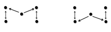
Figure 1: The communication graph of the HK system alternates between these two configurations.

3 An Overview of the Proof

Given the challenge of presenting the multiple threads of the argument in digestible form, we begin with a bird’s eye view of the proof. The standard way to establish the convergence of an algorithm or a dynamical system is to focus on a single unknown input and track the rate at which the system expends a certain resource on its way toward equilibrium: a potential function in algorithms; a free energy in statistical physics; or a Lyapunov function in dynamics. This approach cannot work here. Instead, we need to study the system’s action on all inputs at once. This is probably the single most important feature distinguishing natural algorithms from the classical kind: because they run forever, qualitative statements about their behavior will sometimes require a global view of the algorithm’s actions with respect to all of its inputs. For this, we need a language that allows us to model the evolution of phase space as a single geometric object. This is our next topic. As explained earlier, we may assume that $d=1$.

The coding tree.

This infinite rooted tree encodes into one geometric object the set of all orbits and the full symbolic dynamics. It is the system’s “Rosetta stone,” from which everything of interest can be read off. The coding tree ${\mathcal{T}}$ is embedded in $\Omega^{n}\times{\mathbb{R}}$, where $\Omega=(0,1)$ and the last dimension represents time. Each child $v$ of the root is associated with an atom $U_{v}$, while the root itself stands for the phase space $\Omega^{n}$. The phase tube $(U_{v},V_{v})$ of each child $v$ is the “time cylinder” whose cross-sections at times $0$ and $1$ are $U_{v}$ and $V_{v}=f(U_{v})$, respectively. In general, a phase tube is a discontinuity-avoiding sequence of iterated images of a given cell in phase space. The tree is built recursively by subdividing $V_{v}$ into the cells $c$ formed by its intersection with the atoms, and attaching a new child $w$ for each $c$: we set $V_{w}=f(c)$ and $U_{w}=U_{v}\cap f^{-t_{v}}(c)$, where $t_{v}$ is the depth of $v$ (Fig. 2). The phase tube $(U_{v},V_{v})$ consists of all the cylinders whose cross-sections at $t=0,\ldots,t_{v}$ are, respectively, $U_{v},f(U_{v}),\ldots,f^{t_{v}}(U_{v})=V_{v}$. Intuitively, ${\mathcal{T}}$ divides up the phase space into maximal regions over which the iterated map is linear.

The coding tree has three structural parameters that require investigation. One of them is combinatorial. Label each node $w$ of the tree by the unique atom that contains the cell $c$ defined above. This allows us to interpret any path as a word of atom labels and define the language $L({\mathcal{T}})$ of all such words: the word-length growth of $L({\mathcal{T}})$ plays a central role, which we capture with the word-entropy (formal definitions below). The two other parameters are geometric: the thinning rate tells us how fast the tree’s branches thin out; the attraction rate tells us how close to “periodic” the branches become. Whereas the latter concerns the behavior of single orbits, the thinning rate indicates how quickly a ball in the space of orbits contracts with time, or equivalently how quickly the distribution of agent positions loses entropy.

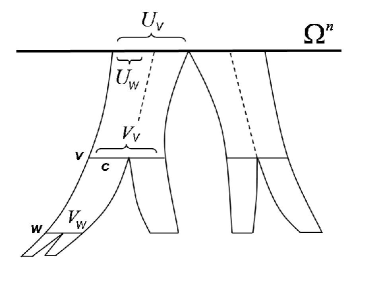
Figure 2: Node $w$ at depth $t_{w}=2$ in the coding tree, with its phase tube $(U_{w},V_{w})$ (curved for aesthetic reasons). The cell $U_{w}$ lies within a single atom whereas $V_{w}$ splits over two of them. Time points downwards. We have represented only two of the possibly many children of the root.

How do we read periodicity off from the coding tree? Intuitively, one would expect that, at some time $\nu$ called the nesting time, for every $v$ of depth $t_{v}=\nu$, there exists $w$ at the same depth with $V_{v}\subseteq U_{w}$. In other words the bottom sections of the phase tubes will, suitably permuted, fit snugly within the top sections. This is not always true, however, and to find necessary conditions for it necessitates a delicate bifurcation analysis. Fig. 3 suggests a visual rule-of-thumb to guide our intuition in distinguishing between chaos and periodicity: the set ${\mathcal{R}}$ consists of the points in phase space where the map $f$ is not continuous.

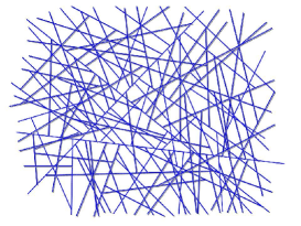
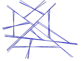
Figure 3: Two scenarios for the iterated preimages of the SP discontinuities ${\mathcal{R}}$: the set ${\mathcal{R}}\cup f^{-1}({\mathcal{R}})\cup\cdots\cup f^{-t}({\mathcal{R}})$ depicted on the left seems to spread everywhere in phase space so as to cover all of it eventually, a symptom of chaos; the set on the right tends to fall into clusters or escape outside of $\Omega^{n}$, a sign of periodicity.

The algorithmic pipeline.

We assemble the coding tree by glueing together smaller coding trees defined recursively. We entrust this task to the arborator, an algorithm expressed in a language for “lego-like” assembly. The arborator needs two (infinite) sets of parameters to do its job, the coupling times and the renormalization scales. To produce these numbers, we use the flow tracker, an algorithm that, in the bidirectional case, works roughly like this: (i) declare agent 1 wet; (ii) any dry agent becomes wet as soon as it links to a wet one; (iii) if all agents ever become wet, dry them all and go back to (i). The instants $t_{k}$ at which wetness propagates constitute the coupling times; the renormalization scales are given by the number $w_{k}$ of wet agents at time $t_{k}$. The key idea is that, between two coupling times $t_{k}$ and $t_{k+1}$, the system breaks up into two subsystems with interaction between them going only in one direction: from wet to dry. We denote by ${\mathcal{A}}(p\rightarrow q)$ an influence system that consists of two groups of size $p$ and $q$, with none of the $q$ agents ever linking up to any of the $p$ agents. This allows us a recursive decomposition of the overall system:

${\mathcal{A}}(n\rightarrow 0)$

For $k=1,2,\ldots$

• Run ${\mathcal{A}}(w_{k}\rightarrow n-w_{k})$ and ${\mathcal{A}}(n-w_{k}\rightarrow 0)$ concurrently between times $t_{k}$ and $t_{k+1}$.

This formulation is of interest only if we can bound $t_{k+1}-t_{k}$. This is done implicitly by recursively monitoring the long-term behavior of the two subsystems and inferring from it the possibility of further wetness propagation. The flow tracker is a syntactical device because it merely monitors the exchange of information among agents with no regard for what is done with it. By contrast, the arborator models the agents’ interpretation of that information into a course of action. The arborator is assembled as a recursive arithmetic expression over four operations: $\oplus$, $\otimes$, absorb, and renorm (Fig. 4). It comes with a dictionary that spells out the effect of each term on the coding tree’s structural parameters. Here is a quick overview:

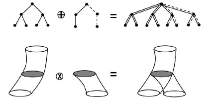
Figure 4: The two tensor products.

• The direct sum $\oplus$ models the parallel execution of two independent subsystems. Think of two agents, Bob and Alice, interacting with each other in one corner of the room while Carol and David are chatting on the other side. The coding tree of the whole is the (pathwise) Cartesian product of both two-agent coding trees.

• The direct product $\otimes$ performs tree surgery. It calls upon another primitive, absorb, to prune the trees and prepare their phase tubes for “glueing.” Imagine Alice suddenly turning to Carol and addressing her. The flow tracker records that the two groups, Bob-Alice and Carol-David, are no longer isolated. Since this might not have happened had Alice been at a slightly different location, the phase tube leading to this event may well split into two parts: one bearing witness to the new interaction; and the other extending the direct sum unchanged. By analogy with the addition of an absorbing state to a Markov chain, the first operation is called absorb.

• The primitive renorm, so named for its kinship with the renormalization group of statistical physics, uses the renormalization scales to compress subtrees into single nodes so as to produce (nonuniform) time rescaling.

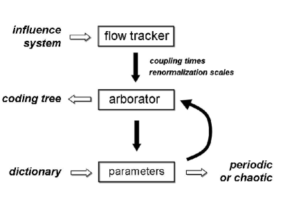
Figure 5: Given the specification of the natural algorithm, the flow tracker computes the coupling times and the renormalization scales, which are needed by the arborator to assemble the coding tree. A dictionary allows us to bound the coding tree’s structural parameters by examining the arborator one component at a time. Renormalization makes this a recursive process, hence the loop between the arborator and the parameters box.

Attraction and chaos.

The occurrence of chaos is mediated by the tension between two forces: dissipation causes the phase tubes to become thinner, which favors periodicity; phase tube splitting produces a form of expansion conducive to chaos. Two arbitrarily close orbits can indeed diverge wildly once they fall on both sides of a discontinuity. The phase tubes snake around phase space while getting thinner at an exponential rate, so hitting SP discontinuities should become increasinly rare over time. The problem is that branching multiplies the chances of hitting discontinuities. For dissipation to overcome branching, the average node degree should be small. To show this is indeed the case requires a fairly technical rank argument about the linear constraints implied by the splitting of a phase tube.

The thinning rate is about contraction, not attraction. To see why, consider a trivial system with only self-loops: it is stuck at a fixed point, yet the agents’ marginal distributions suffer no loss of entropy. The information-theoretic interpretation of thinning is illuminating. As agents are attracted to a limit cycle, they lose memory of where they came from, something that would not happen in a chaotic system. Paradoxically, interaction can then act as a memory recovery device and thus delay the onset of periodicity.

Say the group Alice-Bob-Carol is isolated from David, until the latter decides to interact with Alice, thus taking in a fixed fraction of her entropy. Fast-forward. Alice is now caught in a limit cycle with Bob and Carol, while David has yet to interact with anyone since his earlier contact with Alice. His isolation means that he has had no chance to shed any of Alice’s entropy. Although later caught in a periodic orbit, Alice might still be subject to tiny fluctuations, leading to a sudden interaction with David. When this happens, she will recapture part of the entropy she had lost: she will recover her memory! Happy as the news might be to her, this only delays the inevitable, which is being caught yet again in a limit cycle. Memory recovery cannot recur forever because David loses some of his own memory every time. In the end, because of dissipation, all the agents’ memory will be lost.

4 Algorithmic Dynamics

We flesh out the ideas above, beginning with a simple local characterization of periodicity. We then proceed to define the coding tree (§4.2), the arborator (§4.3), and the flow tracker (§4.4).

4.1 Conditions for asymptotic periodicity

It is convenient to thicken the discontinuities. This does not change the dynamics of the system and is used only as an analytical device. Fix a small parameter $\varepsilon>0$ once and for all, and, for any $t\geq 0$, define the margin ${\mathcal{R}}_{\varepsilon}$, where

$${\mathcal{R}}_{\varepsilon}=\bigcup_{\text{\em SP}}\,\Bigl{\{}\,{\mathbf{x}}=(x_{1},\ldots,x_{n})\in{\mathbb{R}}^{n}\,:\,|\,a_{0}+a_{1}x_{1}+\cdots+a_{n}x_{n}+\delta|\leq\varepsilon\,\Bigr{\}},$$ (1)

where the union extends over all the SP discontinuities. The margin is made of $n^{O(1)}$ closed slabs of width at least $\varepsilon n^{-O(1)}$. It is useful to classify the initial states by how long it takes their orbits to hit ${\mathcal{R}}_{\varepsilon}$, if ever. With $f^{0}={\rm Id}$ and $\min\emptyset=\infty$, we define the label of ${\mathbf{x}}\in\Omega^{n}$ as

$$\ell({\mathbf{x}})=\min\,\Bigl{\{}\,t\geq 0\,|\,f^{t}({\mathbf{x}})\in{\mathcal{R}}_{\varepsilon}\,\Bigr{\}}.$$

The point ${\mathbf{x}}$ is said to vanish at time $\ell({\mathbf{x}})$ if its label is finite. As we shall see, the analysis needs to focus only on the nonvanishing points. Write ${\mathcal{S}}_{t}=\{\,{\mathbf{x}}\in\Omega^{n}=(0,1)^{n}\,|\,\ell({\mathbf{x}})\geq t\,\}$ for the set of points that do not vanish before time $t$: ${\mathcal{S}}_{0}$ is $\Omega^{n}$; and, for $t>0$,

$${\mathcal{S}}_{t}=\Omega^{n}\setminus\bigcup_{k=0}^{t-1}f^{-k}({\mathcal{R}}_{\varepsilon})\,.$$

Each of its connected components is specified by a set of strict linear inequalities in ${\mathbb{R}}^{n}$, so ${\mathcal{S}}_{t}$ is a union of disjoint open $n$-cells, whose number we denote by $\#{\mathcal{S}}_{t}$. We redefine an atom to be a cell of ${\mathcal{S}}_{1}$ and restrict the domain of $f$ to these new atoms. Each cell of ${\mathcal{S}}_{t+1}$ lies within a cell of ${\mathcal{S}}_{t}$. The limit set ${\mathcal{S}}_{\infty}=\bigcap_{\,t\geq 0}{\mathcal{S}}_{t}$ collects the points that never vanish. Unlike those of ${\mathcal{S}}_{t}$, its cells may not be open or full-dimensional.

Periodic sofic shifts.

Any cell $c$ of ${\mathcal{S}}_{\infty}\subseteq{\mathcal{S}}_{1}$ lies within a single atom, so we can define $f_{|c}$ as the linear map corresponding to the transition matrix $P_{c}$. Since ${\mathcal{S}}_{\infty}$ is an invariant set, the image $f(c)$ must, by continuity, lie entirely within a cell of ${\mathcal{S}}_{\infty}$. Suppose that $\#{\mathcal{S}}_{\infty}<\infty$, a fact we will prove shortly. We define a directed graph $F$, with each node labeled by a cell $c$ of ${\mathcal{S}}_{\infty}$ and with an edge $(c,c^{\prime})$, labeled by $f_{|c}$, joining $c$ to the unique cell $c^{\prime}$ of ${\mathcal{S}}_{\infty}$ that contains $f(c)$. The system forms a sofic shift (ie, a regular language over the edge labels). Furthermore, $F$ is functional, meaning that each node has exactly one outgoing edge (possibly a self-loop), so any infinite path ends up in a cycle. The trajectory of a point ${\mathbf{x}}$ is the string $s({\mathbf{x}})=c_{0}c_{1}\cdots$ of atoms that it visits: $f^{t}({\mathbf{x}})\in c_{t}$ for all $0\leq t<\ell({\mathbf{x}})$. It is infinite if and only if ${\mathbf{x}}$ does not vanish, so all infinite trajectories are eventually periodic. The weakness of this result is that it might be a statement about the empty set. To strengthen it, we declare the system to be nesting at $t$ if no cell $c$ of ${\mathcal{S}}_{t}$ contains more than one cell of ${\mathcal{S}}_{t+1}$. (This does not mean that $f(c)$ lies inside an atom.) The minimum value of $t$ is called the nesting time $\nu$ of the system. Observe that $\#{\mathcal{S}}_{\nu}\geq\#{\mathcal{S}}_{t}$, for any $t\geq\nu$. We bound the nesting time and then proceed with an alternative characterization of nesting.

Lemma 4.1

$\!\!\!.\,\,$ Both the nesting time $\nu$ and the number of cells in ${\mathcal{S}}_{t}$ are bounded by $(n/\varepsilon)^{O(n)}$, for $t=0,1,\ldots,\infty$.

Proof. We begin with the second claim. If, in (1), we replace ${\mathbf{x}}$ by $P{\mathbf{x}}$, for a stochastic matrix $P$, the coefficients of the affine form remain polynomially bounded, so the cells of ${\mathcal{S}}_{t}$ are separated from one another by slabs of thickness at least $\varepsilon n^{-O(1)}$. A simple volume argument implies an upper bound of $(n/\varepsilon)^{O(n)}$ on the number of such cells. To bound the nesting time, consider this procedure: suppose that we have placed a special point (called a witness) in each cell $c$ of ${\mathcal{S}}_{t}$. If $c$ contains only one cell of ${\mathcal{S}}_{t+1}$, we move its witness to that unique cell; if it contains more than one cell, then we move the witness to one of them and create new witnesses to supply the others; if $c$ contains no cell of ${\mathcal{S}}_{t+1}$, we leave its witness in place. We carry out this process for $t=0,1,\ldots$, beginning with a single witness in ${\mathcal{S}}_{0}$. Witnesses may move around but never disappear; furthermore, by the previous argument, any two of them are separated by at least $\varepsilon n^{-O(1)}$, so their number is bounded by $(n/\varepsilon)^{O(n)}$. Any time $t$ at which the system fails to be nesting sees the creation of at least one new witness, and the first claim follows. $\Box$

Lemma 4.2

$\!\!\!.\,\,$ Given any cell $c$ of ${\mathcal{S}}_{t}$ and $k\leq t$, the function $f_{|c}^{k}$ is linear. Given any cell $b\subseteq\Omega^{n}$ and any linear function $g$, if $g(b)\setminus{\mathcal{R}}_{\varepsilon}$ is connected then so is $b\setminus g^{-1}({\mathcal{R}}_{\varepsilon})$.

Proof. To call $f_{|c}^{k}$ linear is to say that $f^{k}$ is described by a single stochastic matrix over all of $c$. We may assume that $t>0$. Given a cell $c\subseteq{\mathcal{S}}_{t}$, none of the cells $c,f(c),\ldots,f^{t-1}(c)$ intersect ${\mathcal{R}}_{\varepsilon}$, hence each one falls squarely within a single atom and $f_{|c}^{k}$ is linear for any $k\leq t$. For the second claim, note that, if the cell $b$ intersects more than one connected component of $\Omega^{n}\setminus g^{-1}({\mathcal{R}}_{\varepsilon})$, then it contains a segment $pq$ and a point $r\in pq$ such that $g$ maps $p$ and $q$ outside of ${\mathcal{R}}_{\varepsilon}$ and $r$ inside of it. By linearity, $g(r)$ lies on the segment $g(p)g(q)$; therefore $g(b)\setminus{\mathcal{R}}_{\varepsilon}$ is nonconvex hence disconnected. $\Box$

Lemma 4.3

$\!\!\!.\,\,$ The nesting time $\nu$ is the minimum $t$ such that $f^{t}(c)\setminus{\mathcal{R}}_{\varepsilon}$ is connected for each cell $c$ of ${\mathcal{S}}_{t}$; as a corollary, if $c$ is a cell of ${\mathcal{S}}_{\nu}$, then $f(c)$ intersects at most one cell of ${\mathcal{S}}_{\nu}$.

Proof. The claims are trivial if $\nu=0$, so assume that $\nu>0$. For the first claim, it suffices to show that the system is nesting at time $t>0$ if and only if $f^{t}(c)\setminus{\mathcal{R}}_{\varepsilon}$ is connected for each cell $c$ of ${\mathcal{S}}_{t}$. For the “only” part, we show why $f^{t}(c)\setminus{\mathcal{R}}_{\varepsilon}$ must be connected. By Lemma 4.2, $f^{t}_{|c}$ is linear; therefore, since $c^{\prime}=c\setminus f^{-t}({\mathcal{R}}_{\varepsilon})$ is connected so is $f^{t}(c^{\prime})=f^{t}(c)\setminus{\mathcal{R}}_{\varepsilon}$. Conversely, assuming that each set $f^{t}(c)\setminus{\mathcal{R}}_{\varepsilon}$ is connected, then we identify the function $g$ in Lemma 4.2 with $f^{t}_{|c}$ (in its linear extension) and conclude that $c\setminus g^{-1}({\mathcal{R}}_{\varepsilon})=c^{\prime}$ is connected, hence constitutes the sole cell of ${\mathcal{S}}_{t+1}$ lying within $c$. To prove the corollary, again we turn to Lemma 4.2 to observe that $f_{|c},\ldots,f^{\nu}_{|c}$ are all linear, hence so is $g=f^{\nu-1}_{|b}$, for $b=f(c)$. Our new characterization of nesting implies that $f^{\nu}(c)\setminus{\mathcal{R}}_{\varepsilon}=g(b)\setminus{\mathcal{R}}_{\varepsilon}$ is connected, hence so is $b\setminus g^{-1}({\mathcal{R}}_{\varepsilon})=f(c)\setminus f^{1-\nu}({\mathcal{R}}_{\varepsilon})$. Since $f(c)$ lies entirely within a cell of ${\mathcal{S}}_{\nu-1}$, the labels of its points are all at least $\nu-1$. Removing from $f(c)$ the points of label $\nu-1$ leaves the connected set $f(c)\setminus f^{1-\nu}({\mathcal{R}}_{\varepsilon})$; therefore, $f(c)$ can intersect at most one cell of ${\mathcal{S}}_{\nu}$. $\Box$

We define the directed graph $F$ with one node per cell $c$ of ${\mathcal{S}}_{\nu}$ and an edge from $c$ to $c^{\prime}$, where $c^{\prime}$ is the unique cell of ${\mathcal{S}}_{\nu}$, if it exists, that intersects $f(c)$. Every trajectory corresponds to a directed path in $F$. The main difference with the previous graph is that the converse is not true. Not only a node may lack an outgoing edge but, worse, nothing in this framework keeps an orbit from going around a cycle for a while only to vanish later. The previous lemma’s failure to ensure that $f(c)$ lies strictly within another cell of $S_{\nu}$ puts periodicity in jeopardy. Perturbation is meant to get around that difficulty. Periods and preperiods are defined with respect to the paths of $F$, not trajectories: since the correspondence from paths to trajectories is not injective, the latter may have shorter periods.

Lemma 4.4

$\!\!\!.\,\,$ The system is nesting at $\nu$ and any time thereafter. Any nonvanishing orbit is eventually periodic and the sum of its period and preperiod is bounded by $\#{\mathcal{S}}_{\nu}$.

The attraction rate.

Assume that $\nu>0$ and let $c$ be a cell of ${\mathcal{S}}_{\nu}$. Identifying the nodes of $F$ with their cells in ${\mathcal{S}}_{\nu}$, we denote by $\sigma_{0},\sigma_{1},\ldots$ the path from $c=\sigma_{0}$. Let $j$ be the smallest index such that $\sigma_{i}=\sigma_{j}$ for some $i<j$. This defines the period $p=p(c)=j-i$ and the preperiod $q=q(c)=i$, with $p+q\leq\#{\mathcal{S}}_{\nu}$. Given any ${\mathbf{x}}\in c$, its trajectory $s({\mathbf{x}})=c_{0}c_{1}\cdots c_{\ell({\mathbf{x}})-1}$ is such that $c_{k}$ is the atom containing the cell $\sigma_{k}$. Furthermore, for any $q\leq t\leq\ell({\mathbf{x}})$,

$$f^{t}({\mathbf{x}})=M_{t-q\,(\text{\scriptsize mod}\,p)}\,Q^{\lfloor(t-q)/p\rfloor}f^{q}({\mathbf{x}}),$$ (2)

where $M_{k}=P_{c_{q+k-1}}\cdots P_{c_{q}}$, for $k=0,\ldots,p-1$, and $Q=M_{p}$, with $M_{0}$ the identity matrix. Because of the self-loops in the communication graphs, the powers of $Q$ are known to converge to a matrix $\widetilde{Q}$ [50]. Given $c$ and $t\geq 0$, we define

$$\Pi_{\,t}=M_{t-q\,(\text{\scriptsize mod}\,p)}\,\widetilde{Q}\,P_{c_{q-1}}\cdots P_{c_{0}}.$$

The approximation $\Pi_{t}$ is one of $p$ matrices obtained by substituting $\widetilde{Q}$ for as many “chunks” $Q=M_{p}$ we can extract from the matrix product $P_{c_{t-1}}\cdots P_{c_{0}}$ that defines $f_{|c}$. Note that this includes the case $t<p+q$, where no such chunk is to be found. Given any real $\alpha>0$, we define the attraction rate $\theta_{\alpha}$ as the maximum value of $\theta_{\alpha}(c)$, over all cells $c$ of ${\mathcal{S}}_{\nu}$, where

$$\begin{split}\theta_{\alpha}(c)=\min\,\Bigl{\{}\,\theta\geq 0\,:\,&\|f^{t}({\mathbf{x}})-\Pi_{\,t(\text{\scriptsize mod}\,p)}\,{\mathbf{x}}\|_{\infty}\leq\,\alpha\,,\\ &\hskip 56.9055pt\text{ for all ${\mathbf{x}}\in c$}\,\,\,\text{and}\,\,\,\theta\leq t\leq\ell({\mathbf{x}})\,\Bigr{\}}.\end{split}$$ (3)

Suppose that $Q$ can be written as

$$Q=\begin{pmatrix}A&C\\ \emptyset&B\end{pmatrix}$$ (4)

and assume the existence of a limit matrix $\widetilde{B}$ such that $\|B^{t}-\widetilde{B}\|_{\text{max}}\leq e^{-\gamma t}$, for some $\gamma>0$. We tie the attraction rate to the maximum row-sum in $A$, which is itself related to the thinning rate (whose formal definition we postpone).

Lemma 4.5

$\!\!\!.\,\,$ Given $Q$ as in (4) and an upper bound $\mu$ on $\|A\,{\mathbf{1}}\|_{\infty}$ such that $e^{-\gamma}\leq\mu<1$, for any $0<\alpha<1-\mu$,

$$\theta_{\alpha}=O\Bigl{(}\,\frac{\#{\mathcal{S}}_{\nu}}{1-\mu}\,\Bigr{)}\log\hbox{$\frac{n}{\alpha}$}\,.$$

Proof. For any $t>0$,

$$Q^{t}=\begin{pmatrix}A^{t}&C_{t}\\ 0&B^{t}\end{pmatrix}.$$

The matrix $A$ is strictly substochastic ($\mu<1$), so, by standard properties of a Markov chain’s fundamental matrix, $\sum_{k\geq 0}A^{k}=(I-A)^{-1}$; therefore, for $t>0$,

$$C_{t}-(I-A^{t})(I-A)^{-1}C\widetilde{B}=\sum_{k=0}^{t-1}A^{t-k-1}CB^{k}-\sum_{k=0}^{t-1}A^{k}C\widetilde{B}\\ =\sum_{k=0}^{t-1}A^{t-k-1}CD_{k},$$

where $D_{k}=B^{k}-\widetilde{B}$. Since $C$ is substochastic, $\|CD_{k}\|_{\text{max}}\leq e^{-\gamma k}$. From $\|A^{k}\,{\mathbf{1}}\|_{\infty}\leq\mu^{k}$, we derive

$$\|A^{t-k-1}CD_{k}\|_{\text{max}}\leq\mu^{t-k-1}e^{-\gamma k}.$$

Since $\mu\geq e^{-\gamma}$, it follows that $\|C_{t}-(I-A^{t})(I-A)^{-1}C\widetilde{B}\|_{\text{max}}\leq t\mu^{t-1}$; hence,

$$\widetilde{Q}=\begin{pmatrix}0&(I-A)^{-1}C\widetilde{B}\,\\ 0&\widetilde{B}\end{pmatrix},$$

where, by $\|A^{t}\|_{\text{max}}\leq\mu^{t}$ and $\|(I-A)^{-1}\|_{\text{max}}\leq 1/(1-\mu)$, $\|Q^{t}-\widetilde{Q}\|_{\text{max}}=O(tn\mu^{t-1}/(1-\mu))$. As a result, by Lemma 4.4, $\theta_{\alpha}\leq q+pt\leq(\#{\mathcal{S}}_{\nu})t$, if $t$ satisfies $t\mu^{t-1}<\alpha(1-\mu)n^{-b}$, for a large enough constant $b>0$. $\Box$

This next result argues that, although a vanishing point may take arbitrarily long to do so, it comes close to vanishing fairly early. This gives us a useful analytical device to avoid summing complicated series when estimating the probability that a point will eventually vanish under random margin perturbation.

Lemma 4.6

$\!\!\!.\,\,$ Given any finitely-labeled point ${\mathbf{x}}$ in a cell $c$ of ${\mathcal{S}}_{\nu}$, there exists $t<\theta_{\alpha}+p(c)+q(c)$ such that $f^{t}({\mathbf{x}})\in{\mathcal{R}}_{2\varepsilon}$, for some $\alpha\geq\varepsilon n^{-O(1)}$.

Proof. We can obviously assume that $\ell({\mathbf{x}})\geq\theta_{\alpha}+p(c)+q(c)$. For any $t$ such that $\theta_{\alpha}\leq t\leq\ell({\mathbf{x}})$, $f^{t}({\mathbf{x}})$ lies in an $\ell_{\infty}$ ball of radius $\alpha$ centered at $\Pi_{\,t\,\text{\scriptsize mod}\,p(c)}\,{\mathbf{x}}$. This means that, between times $\theta_{\alpha}+q(c)$ and $\ell({\mathbf{x}})$, the orbit of ${\mathbf{x}}$ lies entirely in the union of $p(c)$ balls of radius $\alpha$ and, by periodicity, each ball is visited before time $\theta_{\alpha}+p(c)+q(c)$. Since ${\mathbf{x}}$ vanishes at time $\ell({\mathbf{x}})$, one of these $p(c)$ balls must intersect ${\mathcal{R}}_{\varepsilon}$. Thickening all the margin slabs by a width of $4\alpha\sqrt{n}$ is enough to cover that ball entirely. If $\alpha=\varepsilon n^{-b}$ for a large enough constant $b$, replacing $\varepsilon$ by $2\varepsilon$ achieves the required thickening. $\Box$

Although nesting occurs within finite time, the strict inclusion ${\mathcal{S}}_{k+1}\subset{\mathcal{S}}_{k}$ may occur infinitely often. We show why:

Example 4.1: Vanishing can take arbitrarily long. Consider the two-agent influence system

$$\begin{pmatrix}x_{1}\\ x_{2}\end{pmatrix}\,\stackrel{{\scriptstyle f}}{{\longmapsto}}\,\hbox{$\frac{1}{3}$}\begin{pmatrix}2&1\\ 1&2\end{pmatrix}\begin{pmatrix}x_{1}\\ x_{2}\end{pmatrix},$$

with the SP discontinuities formed by the single slab

$${\mathcal{R}}_{\varepsilon}=\{\,{\mathbf{x}}\in{\mathbb{R}}^{3}\,:\,|x_{1}-1+\delta|\leq\varepsilon\,\}.$$

For simplicity, assume the same linear map $f$ in the two atoms. It follows that

$$\begin{pmatrix}x_{1}\\ x_{2}\end{pmatrix}\,\stackrel{{\scriptstyle f^{t}}}{{\longmapsto}}\,\hbox{$\frac{1}{2}$}\begin{pmatrix}1+3^{-t}&1-3^{-t}\\ 1-3^{-t}&1+3^{-t}\end{pmatrix}\begin{pmatrix}x_{1}\\ x_{2}\end{pmatrix}.$$

The set ${\mathcal{S}}_{\infty}$ is the complement within $\Omega^{2}$ (the effective phase space) of

$$\bigcup_{t=0}^{\infty}\,\Bigl{\{}\,|\,(1+3^{-t})X_{1}+(1-3^{-t})X_{2}-2+2\delta\,|\leq 2\varepsilon\,\Bigr{\}}.$$

Note that if $\varepsilon=0$, the number of cells in ${\mathcal{S}}_{\infty}$ is infinite: they are defined by an infinite number of lines passing through $(1-\delta,1-\delta)$, with increasing slopes tending to $-1$. As soon as we allow thickness $\varepsilon>0$, however, the margin creates only $O(|\!\log\varepsilon|)$ cells. Not all of them are open. To see this, consider the point $2(1-\delta+\varepsilon,0)$. It never vanishes yet any neighborhood contains points that do. Some points take arbitrarily long to vanish. Thickening the SP discontinuities into slabs is a “finitizing” device meant to keep the number of $\infty$-labeled cells bounded.

4.2 The coding tree

The richly decorated tree ${\mathcal{T}}$ encodes the branching structure of the sets ${\mathcal{S}}_{k}$ as a geometric object in “phase space $\times$ time” $=\Omega^{n}\times[0,\infty)$. Recall that each atom $c$ comes with its own transition matrix $P_{c}$. Unless specified otherwise, a fixed perturbation value of $\delta$ is assumed once and for all. Think of $U_{v}$ and $V_{v}$ as the end-sections at times $0$ and $t_{v}$ of a phase tube containing all the orbits originating from $U_{v}$. At time $t_{v}$, the SP discontinuities might split the tube. This happens only if $V_{v}$ intersects the margin, which is the “branching condition” in the boxed algorithm. That intersection indicates the vanishing time of some points in $U_{v}$, so we place a leaf as an indicator, and call it a vanishing node. Whereas $U_{v}$ is an open $n$-cell, $V_{v}$ can be a cell of any dimension; hence so can be the connected components of $V_{v}\setminus{\mathcal{R}}_{\varepsilon}$. For each one, $c$, we attach a new child $w$ to $v$ and denote by $P_{w}$ the matrix of the map’s restriction to $c$. The image of $c$ at time $t_{v}$, ie, $P_{w}\,c$, forms the end-section $V_{w}$ of a new phase tube from the root, whose starting section $U_{w}$ is the portion of $U_{v}$ mapping to $c$ at time $t_{v}$ (Fig. 2).

Building ${\mathcal{T}}$

• The root $v$ has depth $t_{v}=0$; set $U_{v}\leftarrow V_{v}\leftarrow\Omega^{n}$.

• Repeat forever:

  • For each newly created node $v$:

    • If $V_{v}\cap{\mathcal{R}}_{\varepsilon}\neq\emptyset$                  [ branching condition ]
      then create a leaf and make it a child of $v$.

    • For each cell $c$ of $V_{v}\setminus{\mathcal{R}}_{\varepsilon}$, create a child $w$ of $v$ and
      set $P_{w}\leftarrow P_{c}$ ;   $V_{w}\leftarrow P_{w}\,c$ ;   $U_{w}\leftarrow U_{v}\cap f^{-t_{v}}(c)$.

Let $ww^{\prime}w^{\prime\prime}\cdots$ denote the upward, $t_{w}$-node path from $w$ to the root (but excluding the root). Using the notation $P_{\leq w}=P_{w}P_{w^{\prime}}P_{w^{\prime\prime}}\cdots$, we have the identity $V_{w}=P_{\leq w}\,U_{w}$. No point in $U_{w}$ vanishes before time $t_{w}$, and, in fact, ${\mathcal{S}}_{k}=\bigcup_{w}\{\,U_{w}\,|\,t_{w}=k\,\}$. The points of ${\mathcal{S}}_{\infty}$ are precisely those whose orbits follow an infinite path $v_{\infty}=v_{0},v_{1},v_{2},\ldots$ down the coding tree. Each such path has its own limit cell $U_{v_{\infty}}=\bigcap_{\,t\geq 0}U_{v_{t}}$: collectively, these form the cells of ${\mathcal{S}}_{\infty}$. Example 4.1 features two infinite paths each of whose nodes has two children, one vanishing and one not.

• The nesting time $\nu=\nu({\mathcal{T}})$ is the minimum depth at which any node has at most one nonvanishing child (Lemma 4.3); visually, below depth $\nu$, the tree consists of single paths, some finite, others infinite, with vanishing leaves hanging off some of them. A node $v$ is deep if $t_{v}>\nu$ and shallow otherwise.

• The word-entropy $h({\mathcal{T}})$ is the logarithm of the number of shallow nodes. As we observed, ${\mathcal{S}}_{\nu}=\bigcup_{v}\{\,U_{v}\,|\,t_{v}=\nu\,\}$; therefore $\#{\mathcal{S}}_{\nu}\leq 2^{h({\mathcal{T}})}$.

• The period $p({\mathcal{T}})$ is the maximum value of $p(c)$ for all cells $c=U_{v}$, with $t_{v}=\nu$. The attraction rate $\theta_{\alpha}({\mathcal{T}})$ is the maximum value of the attraction rate for any such $c$.

The global coding tree.

Let ${\mathbb{I}}$ denote the interval $[-1,1]$. Since not all perturbations $\delta$ are equally good, we must understand how the coding tree ${\mathcal{T}}$ varies as a function of $\delta$. To do that, a global approach is necessary: given $\Delta\subseteq{\mathbb{I}}$, we encode the coding trees for all $\delta\in\Delta$ into a single one, ${\mathcal{T}}^{\Delta}$, which can be viewed as the standard coding tree for the augmented $(n+1)$-dimensional system $({\mathbf{x}},\delta)\mapsto(f({\mathbf{x}}),\delta)$, with the phase space $\Omega^{n}\times\Delta$. The sets $U_{v}$ and $V_{v}$ are now cells in ${\mathbb{R}}^{n+1}$. In the branching condition, one should replace the margin ${\mathcal{R}}_{\varepsilon}$, as defined in (1), by the global margin:

$$\bigcup_{\text{\em SP}}\,\Bigl{\{}\,({\mathbf{x}},\delta)\in{\mathbb{R}}^{n+1}\,:\,|a_{0}+a_{1}x_{1}+\cdots+a_{n}x_{n}+\delta|\leq\varepsilon\,\Bigr{\}}.$$ (5)

The degree of any node is bounded by $n^{O(n)}$, which is the maximum number of cells in an arrangement of $n^{O(1)}$ hyperplanes in ${\mathbb{R}}^{n+1}$. The definition of nesting can be extended, unchanged, to this lifted system. Since a standard coding tree is just a “cross-section” of the global one, nesting in ${\mathcal{T}}$ even for all $\delta$ does not imply nesting in ${\mathcal{T}}^{\Delta}$. The global word-entropy $h({\mathcal{T}}^{\Delta})$ is defined in the obvious way.

4.3 The arborator

This algorithm assembles the coding tree by glueing smaller pieces together. It relies on a few primitives that we now describe. The direct sum and direct product are tensor-like operations used to attach coding trees together. The primitives absorb and renorm respectively prune and compress trees. We present these operations and assemble the dictionary that allows us to bound the coding tree’s parameters as we parse the arborator.

Direct sum.

The coding tree ${\mathcal{T}}={\mathcal{T}}_{1}\oplus{\mathcal{T}}_{2}$ models two independent systems of size $n_{1}$ and $n_{2}$. Independence means that the systems are decoupled (no edge joins agents from distinct groups) and oblivious (no SP discontinuity has nonzero coefficients from both groups): this implies that the two systems can be analyzed separately; decoupling alone is not sufficient. The phase space of the direct sum is of dimension $n=n_{1}+n_{2}$. A path $w_{0},w_{1},\ldots$ of ${\mathcal{T}}$ is a pairing of paths in the constituent trees: the node $w_{t}$ is of the form $(u_{t},v_{t})$, where $u_{t}$ (resp. $v_{t}$) is a node of ${\mathcal{T}}_{1}$ (resp. ${\mathcal{T}}_{2}$) at depth $t$; it is a leaf if and only if $u_{t}$ or $v_{t}$ is one—the vanishing of one group implies the vanishing of the whole. If $w=(u,v)$ is not a leaf, then $U_{w}=U_{u}\times U_{v}$, and $V_{w}=V_{u}\times V_{v}$. The direct sum is commutative and associative. The name comes from the fact that $P_{w}$ is the direct matrix sum of $P_{u}$ and $P_{v}$:

$$P_{w}=P_{u}\oplus P_{v}=\begin{pmatrix}P_{u}&0\\ 0&P_{v}\end{pmatrix}.$$

• Nesting time, period, and attraction rate.

  $$\nu({\mathcal{T}})\leq\,\max_{i=1,2}\,\,\nu({\mathcal{T}}_{i})\hskip 11.38092pt\text{and}\hskip 11.38092ptp({\mathcal{T}})\leq\prod_{i=1,2}\,\,p({\mathcal{T}}_{i})\hskip 11.38092pt\text{and}\hskip 11.38092pt\theta_{\alpha}({\mathcal{T}})\leq\,\max_{i=1,2}\,\,\theta_{\alpha}({\mathcal{T}}_{i}).$$ (6)

  The first two inequalities are obvious, so we focus on the last one. Consider a cell $c=c_{1}\times c_{2}$ of ${\mathcal{S}}_{\nu}$ and follow the path of $F$ emanating from it: this navigation corresponds to the parallel traversal of a path in $F_{i}$ from $c_{i}$—we use the subscript $i=1,2$ to refer to either one of the subsystems. Assume without loss of generality that $q_{1}\geq q_{2}$. By definition, to revisit an earlier node means doing likewise in each traversal; hence $q\geq q_{1}$. At time $q_{1}$, however, both parallel traversals are already engaged in their own respective cycles, so the node pair at time $q_{1}$ will be revisited lcm$\,(p_{1},p_{2})$ steps later, the time span that constitutes the period $p$ of the direct sum; it also follows that $q=q_{1}$. If $q_{1}>q_{2}$, the traversals do not enter their cycles at the same time, so in general, referring to (2), the matrix $Q$ is not the direct sum of $Q_{1}^{p/p_{1}}$ and $Q_{2}^{p/p_{2}}$ but, rather, of a shifted version $Q=Q_{1}^{p/p_{1}}\oplus(BA)^{p/p_{2}}$, where $Q_{2}=AB$. We easily verify that

  $$\widetilde{Q}=\lim_{k\rightarrow\infty}Q^{k}=\widetilde{Q}_{1}\oplus(B\widetilde{Q}_{2}A),$$

  where, as before, $\widetilde{Q}_{i}=\lim_{k\rightarrow\infty}Q_{i}^{k}$. The use of the $\ell_{\infty}$ norm allows us to verify the bound on the attraction rate of the direct sum by checking the accuracy of the approximation for each subsystem separately. It suffices to focus on the case of ${\mathcal{T}}_{2}$, which presents the added difficulty that the approximation scheme delays the cycle entrance until $q_{1}$. The other difference with the approximation scheme in the original system ${\mathcal{T}}_{2}$ is that, since the period can be much longer, so can the sequence $(M_{2})_{k}$. In all cases, however, the approximation scheme in ${\mathcal{T}}$ as it applies to ${\mathcal{T}}_{2}$ differs from the scheme in ${\mathcal{T}}_{2}$ in only one substantive way. Consider the language consisting of the words $(AB)^{*}$, $(AB)^{*}A$, $(BA)^{*}$, and $(BA)^{*}B$. One approximation scheme involves replacing any number of “$AB$”s by $\widetilde{Q}_{2}$, while the other scheme replaces any number of “$BA$”s by $B\widetilde{Q}_{2}A$. Because $AB\widetilde{Q}_{2}=\widetilde{Q}_{2}AB=\widetilde{Q}_{2}$, any application of one scheme or the other produces the same matrix.

• Word-entropy. We prove (quasi) subadditivity. Assume without loss of generality that $\nu({\mathcal{T}}_{1})\geq\nu({\mathcal{T}}_{2})$. The word-entropy counts the number of shallow nodes $w=(u,v)$. This implies that $t_{u}\leq\nu({\mathcal{T}}_{1})$, which limits the number of such nodes $u$ to $2^{h({\mathcal{T}}_{1})}$. If all the nodes $v$ were shallow in ${\mathcal{T}}_{2}$, the subadditivity of word-entropy would be immediate; but it need not be the case. If $v$ is deep, let $s(v)$ be its deepest shallow ancestor. The function $s$ may not be injective but it is at most two-to-one. Thus,

  $$h({\mathcal{T}})\leq h({\mathcal{T}}_{1})+h({\mathcal{T}}_{2})+1.$$ (7)

All of the relations in (6, 7) still hold when the superscript $\Delta$ is added to the coding trees. We discuss (7) to illustrate the underlying principle. First, we provide an independent perturbation variable $\delta_{i}\in\Delta$ to ${\mathcal{T}}_{i}$ ($i=1,2$) and add it as an extra coordinate to the state vector, thus lifting system $i$ to dimension $n_{i}+1$. By (7), the word-entropy of the joint system ${\mathcal{T}}^{*}$ in dimension $n+2$ is at most $h({\mathcal{T}}_{1}^{\Delta})+h({\mathcal{T}}_{2}^{\Delta})+1$. Second, we restrict the system ${\mathcal{T}}^{*}$ to the invariant hyperplane $\delta_{1}=\delta_{2}$, which cannot increase the word-entropy, hence $h({\mathcal{T}}^{\Delta})\leq h({\mathcal{T}}^{*})$, as claimed.

Absorption.

The direct product, which we define below, requires an intermediate construction. The goal is to allow the selection of nodes for removal, with an eye toward replacing the subtrees they root by coding trees with different characteristics. The selection is carried out by an operation called ${\tt absorb}({\mathcal{T}})$, which replaces any deleted node by a leaf. For reasons that the flow tracker will soon clarify, such leaves are designated wet. An orbit that lands into one of these wet leaves is suddenly governed by a different dynamics, modeled by a different coding tree, so from the perspective of ${\mathcal{T}}$ alone, wet leaves are where orbits come to a halt. While vanishing leaves signal the termination of an orbit (at least from the perspective of the analysis), the wet variety merely indicates a change of dynamics. Here is a simple illustration:

Example 4.3: The system consists of two independent subsystems. Suppose we add a union of slabs, denoted by ${\mathcal{R}}_{\varepsilon}^{\prime}$, to the original margin ${\mathcal{R}}_{\varepsilon}^{o}$, thus breaking the direct-sum nature of the coding tree. In Fig. 6, ${\mathcal{R}}_{\varepsilon}^{\prime}$ would consist of the two infinite strips bordering $b$. We keep the transition matrices unchanged everywhere except in cell $b$, which we call wet: all transition matrices are still direct (matrix) sums, with the possible exception of $P_{b}$. Suppose we had available the coding tree prior to the margin’s augmentation. Let $V_{v}$ denote the pentagon in the figure and $w$ be the node associated with the trapezoid $c$ that holds $a,b,d$. We need to replace $w$ by three nodes: two of them for $a,d$ and one, a wet leaf, for $b$. The transition matrices for $a,d$ are both equal to the direct sum $P_{c}$, while $P_{b}$ can be arbitrary. The idea is that $b$ can then be made the region $U_{\text{root}}$ of a new coding tree.

Minor technicality: usually, $U_{\text{root}}=\Omega^{n}$, so the coding tree must be cropped by substituting $b$ for $\Omega^{n}$; note that $b$ need not be an invariant set. Cropping might involve pruning the tree but it cannot increase any of the key parameters, such as the nesting time, the attraction rate, and the period. Absorption appeals to the fact that we can ignore $b$ and its wet leaf until we have fully analyzed the direct sum. This separation is very useful, especially since absorption does not require a direct sum—we never used the fact that the old slabs were horizontal or vertical—and is therefore extremely general.

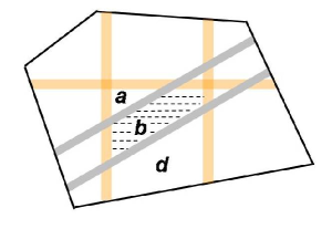
Figure 6: The original cell $c$ of $V_{v}$ (bottom-center trapezoid) splits up into the wet cell $b$ and the dry cells $a$ and $d$, both of which inherit the matrix $P_{c}$.

A crucial observation is that the nodes $z$ created for the subcells $c^{\prime}$ of a given $c$ (subcells $a$ and $d$ in Fig. 6) have the same matrix $P_{c}$. As a result of all the absorptions, the tube $(U_{v},V_{v})$ is split up by up to $t_{v}$ linearly transformed copies of the $n^{O(1)}$ margin slabs, hence into at most $t_{v}^{n}n^{O(n)}$ subcells. This compares favorably with the naive upper bound of $n^{O(nt_{v})}$ based on the sole fact that absorption at each ancestor of $v$ produces $n^{O(n)}$ children.

Absorption surgery

• If $v$ has no leaf, create a vanishing leaf and make it a child of $v$.

• For each cell $c$ of $V_{v}\setminus{\mathcal{R}}_{\varepsilon}^{o}$, let $w$ be the child of $v$ for $c$ (ie, such that $f(c)=V_{w}$) and let $T$ be the tree rooted at $w$. If $c\cap{\mathcal{R}}_{\varepsilon}^{\prime}$, then remove $T$ and, for each cell $c^{\prime}$ of $c\setminus{\mathcal{R}}_{\varepsilon}^{\prime}$, create a node $z$ and make it a child of $v$.

  • If $c^{\prime}$ is wet, make $z$ a wet leaf.

  • If $c^{\prime}$ is dry, reattach to $z$ a suitably cropped copy of $T$.
    Set $P_{z}\leftarrow P_{c}$, $V_{z}\leftarrow P_{z}\,c$, and $U_{z}\leftarrow U_{v}\cap f^{-t_{v}}(c^{\prime})$.

Direct product.

The tree ${\mathcal{T}}={\mathcal{T}}_{1}\otimes{\mathcal{T}}_{2}$ models the concatenation of two systems. The direct product is associative but not commutative. It is always preceded by a round of absorptions at one or several nodes of ${\mathcal{T}}_{1}$. We begin with a few words of intuition. Consider two systems $S_{1}$ and $S_{2}$, governed by different dynamics yet evolving in the same phase space $\Omega^{n}$. Given an arbitrary region $\Lambda\subset\Omega^{n}$, we define the hybrid system $S$ with the dynamics of $S_{2}$ over $\Lambda$ and $S_{1}$ elsewhere. Suppose we had complete knowledge of the coding tree ${\mathcal{T}}_{i}$ for each $S_{i}$ ($i=1,2$). Could we then combine them in some ways to assemble the coding tree ${\mathcal{T}}$ of $S$? To answer this question, we follow a three-step approach:

• (i) we absorb the tree ${\mathcal{T}}_{1}$ by creating wet leaves $w$ for all the nodes $v$ with $V_{v}\cap\Lambda\neq\emptyset$;

• (ii) we attach the roots of cropped copies of ${\mathcal{T}}_{2}$ at the wet leaves; and

• (iii) we iterate and glue ${\mathcal{T}}_{1}$ and ${\mathcal{T}}_{2}$ in alternation, as orbits move back and forth in and out of $\Lambda$.

Absorption, direct products, and the arborator address (i, ii, iii) in that order. The root of ${\mathcal{T}}_{2}$ is attached to $w$, but not until that tree itself has been properly cropped so that $U_{\text{root}}=V_{\text{root}}({\mathcal{T}}_{2})=V_{w}({\mathcal{T}}_{1})=P_{w}\,c$, with $P_{w}$ given by ${\mathcal{T}}_{2}$ and not ${\mathcal{T}}_{1}$. To be fully rigorous, we should write a direct product as ${\mathcal{T}}_{1}\otimes\{{\mathcal{T}}_{2}\}$ since the trees ${\mathcal{T}}_{2}$ we attach to the wet nodes might not all be the same: the cropping might vary, as might the wet regions.

• Nesting time and attraction rate. Bounding the nesting time of a direct product is not merely a combinatorial matter, as was the case for direct sums: the geometry of attraction plays a role. Even the case of ${\tt absorb}({\mathcal{T}}_{1})$ demands some attention and this is where we begin. Adding ${\mathcal{R}}_{\varepsilon}^{\prime}$ to the margin cannot create arbitrarily deep wet nodes: specifically, no $v\in{\tt absorb}({\mathcal{T}}_{1})$ of depth at least $\max\{\,\nu({\mathcal{T}}_{1}),\theta_{\alpha_{a}}({\mathcal{T}}_{1})+p\,\}$ can have a wet child, where $p=p(U_{v})$ and $\alpha_{a}=\varepsilon n^{-a}$ for a large enough constant $a$. Indeed, suppose there is such a node $v$. Pick ${\mathbf{x}}\in U_{v}$ such that $f^{t_{v}}({\mathbf{x}})$ lies in a wet cell $c$ within $V_{v}$ and observe that

  $$\|f^{t_{v}}({\mathbf{x}})-f^{t_{v}-p}({\mathbf{x}})\|_{\infty}\leq\|f^{t_{v}}({\mathbf{x}})-\Pi_{\,t_{v}(\text{\scriptsize mod}\,p)}\,{\mathbf{x}}\|_{\infty}+\|f^{t_{v}-p}({\mathbf{x}})-\Pi_{\,t_{v}(\text{\scriptsize mod}\,p)}\,{\mathbf{x}}\|_{\infty}\leq 2\alpha_{a}.$$

  By our choice of $\alpha_{a}$, this implies that $f^{t_{v}}({\mathbf{x}})$ and $f^{t_{v}-p}({\mathbf{x}})$ are at a distance apart less than the width of the margin’s slabs; therefore, $f^{t_{v}-p}({\mathbf{x}})$ lies in a wet cell or in a slab. It follows that the orbit of ${\mathbf{x}}$ either vanishes or comes to a (wet) halt at a time earlier than $t_{v}$, so ${\mathbf{x}}\not\in U_{v}$ and we have a contradiction. It follows that all deep nodes of ${\mathcal{T}}_{1}$ deeper than $\theta_{\alpha_{a}}({\mathcal{T}}_{1})+p({\mathcal{T}}_{1})$ are also deep in ${\tt absorb}({\mathcal{T}}_{1})$. With ${\mathcal{T}}={\mathcal{T}}_{1}\otimes{\mathcal{T}}_{2}$, therefore,

  $$\begin{cases}\,\,\nu({\tt absorb}({\mathcal{T}}_{1}))\,\leq\max\{\,\nu({\mathcal{T}}_{1}),\,\theta_{\alpha_{a}}({\mathcal{T}}_{1})+p({\mathcal{T}}_{1})\,\}\,,\hskip 8.5359pt\text{for some $\alpha_{a}\geq\varepsilon n^{-O(1)}$}\\ \,\,\nu({\mathcal{T}})\,\leq\,\nu({\tt absorb}({\mathcal{T}}_{1}))+\nu({\mathcal{T}}_{2})\\ \,\,\theta_{\alpha}({\mathcal{T}})\,\leq\max\{\,\theta_{\alpha}({\mathcal{T}}_{1}),\,\nu({\tt absorb}({\mathcal{T}}_{1}))+\theta_{\alpha}({\mathcal{T}}_{2})\,\}\end{cases}$$ (8)

• Word-entropy. Absorption can occur only at nodes $v$ of depth $t_{v}\leq\,\nu({\tt absorb}({\mathcal{T}}_{1}))$. This means that the number of nodes where wet cells can emerge is at most $2^{h({\mathcal{T}}_{1})}(\theta_{\alpha_{a}}({\mathcal{T}}_{1})+p({\mathcal{T}}_{1}))$. As we argued earlier, each such node $v$ can give birth to at most $t_{v}^{n}n^{O(n)}$ new nodes, so the number of shallow nodes in ${\mathcal{T}}$ is (conservatively) at most

  $$\overset{\#v\,\,{\tt with\,\,wet\,\,child}}{\overbrace{\,2^{h({\mathcal{T}}_{1})}(\theta_{\alpha_{a}}({\mathcal{T}}_{1})+p({\mathcal{T}}_{1}))\,}}\times\overset{\#{\tt splits}/v}{\overbrace{\,(\nu({\mathcal{T}}_{1})+\theta_{\alpha_{a}}({\mathcal{T}}_{1})+p({\mathcal{T}}_{1}))^{n}n^{O(n)}\,}}\times\overset{\#{\mathcal{T}}_{2}\,\,{\tt nodes}}{\overbrace{\,2^{h({\mathcal{T}}_{2})}\,}}.$$

  We use the fact that cropping cannot increase the word-entropy. Taking logarithms, we find that

  $$h({\mathcal{T}})\leq h({\mathcal{T}}_{1})+h({\mathcal{T}}_{2})+(n+1)\log(\,\nu({\mathcal{T}}_{1})+\theta_{\alpha_{a}}({\mathcal{T}}_{1})+p({\mathcal{T}}_{1})\,)+O(n\log n).$$ (9)

  Since both $\nu({\mathcal{T}}_{1})$ and $p({\mathcal{T}}_{1})$ are no greater than $2^{h({\mathcal{T}}_{1})}$, we can simplify the bound:

  $$h({\mathcal{T}})\leq(n+2)h({\mathcal{T}}_{1})+h({\mathcal{T}}_{2})+(n+1)\log\theta_{\alpha_{a}}({\mathcal{T}}_{1})+O(n\log n).$$ (10)

We repeat our earlier observation that, by viewing the perturbation variable $\delta$ as an extra coordinate of the state vector, the relations above still hold for global coding trees with $n$ incremented by one.

Renormalization.

This operation is both the simplest and the most powerful in the arborator’s toolkit: the simplest because all it does is compress time by folding together consecutive levels of ${\mathcal{T}}$; the most powerful because it reaches beyond lego-like assembly to bring in the full power of algorithmic recursion into the analysis. The primitive renorm takes disjoint subtrees of ${\mathcal{T}}$ and regards them as nodes of the renormalized tree. This is done in the obvious way: if $u$ is any node in ${\mathcal{T}}$ with two children $v_{1},v_{2}$, each one with two children, $v_{11},v_{12}$ and $v_{21},v_{22}$, then compressing the subtree $u,v_{1},v_{2}$ means replacing it by a node $z$ with the same parent as $u$’s (if any) and the four children $v_{ij}$. We discuss this process in more detail below. Although inspired by the renormalization group of statistical physics, our approach is more general. For one thing, the compressed subtrees may differ in size, resulting in nonuniform rescaling across ${\mathcal{T}}$. This lack of uniformity rules out closed-form composition formulae for the nesting time, attraction rate, and word-entropy of renormalized coding trees, which must then be resolved algorithmically.

4.4 The flow tracker

We approach periodicity through the study of an important family, the block-directional influence systems, whose agents can be ordered so that

$${\mathcal{G}}=\begin{pmatrix}{\mathcal{G}}_{A}&{\mathcal{G}}_{C}\\ 0&{\mathcal{G}}_{B}\end{pmatrix},$$ (11)

where $0$ denotes the $(n-m)$-by-$m$ matrix whose entries are the constant function ${\mathbf{x}}\mapsto 0$; in other words, in a block-directional system, no $B$-agent ever links to an $A$-agent. Suppose that $m<n$. Wet the $B$-agents with water while keeping all the $A$-agents dry. Whenever an edge of the communication graph links a dry agent to a wet one, the former gets wet. Note how water flows in the reverse direction of the edges. As soon as all agents become wet (if ever), dry them but leave the $B$-agents wet, and repeat forever. The case $m=n$ is similar, with one agent designated wet once and for all. The sequence of times at which water spreads or drying occurs plays a key role in building the arborator.

Coupling times and renormalization scales.

Let ${\mathcal{T}}_{m\,\rightarrow\,n-m}$ denote the coding tree of a block-directional system consisting of $m$ (resp. $n-m$) $A$-agents (resp. $B$-agents). The arrow indicates that no $B$-agent can ever link to an $A$-agent: ${\mathcal{G}}_{ij}$ is identically zero for any $B$-agent $i$ and $A$-agent $j$. We use the notation ${\mathcal{T}}_{m\,\|\,n-m}$ for the decoupled case: no edge ever joins the two groups in either direction, but the discontinuities may still mix variables from both groups. Note that the metrical case implies full independence (§1), so that

$${\mathcal{T}}_{m\,\|\,n-m}={\mathcal{T}}_{m}\,\oplus\,{\mathcal{T}}_{n-m}.$$

Assume that $n>1$ and $0<m\leq n$. We write ${\mathcal{T}}_{m\,\rightarrow\,0}$ as ${\mathcal{T}}_{m}$. Likewise, we can always express ${\mathcal{T}}_{m\,\rightarrow\,n-m}$ as ${\mathcal{T}}_{m}$, but doing so is less informative. When the initial state ${\mathbf{x}}$ is undersood, we use the shorthand $G_{t}={\mathcal{G}}(f^{t}({\mathbf{x}}))$ to designate the communication graph at time $t$ and we denote by $W_{t}$ the set of wet agents at that time. The flow tracker is not concerned with information exchanges among the $B$-agents: these are permanently wet and, should they not exist ($m=m$), agent 1 is kept wet at all times [2.1]. Thus the set $W_{t}$ of wet agents is never empty. The assignments of $t_{0}$ in step [2.3] divide the timeline into epochs, time intervals during which either all agents become wet or, failing that, the flow tracker comes to a halt (breaking out of the repeat loop at “stop”). Each epoch is itself divided into subintervals by the coupling times $t_{1}<\cdots<t_{\ell}$, with $W_{t_{k}}\subset W_{t_{k}+1}$. The last coupling time $t_{\ell}$ marks either the end of the flow tracking (if not all $A$-agents become get) or one less than the next value of $t_{0}$ in the loop.

The notion of coupling is purely syntactical, being only a matter of information transfer. Our interest in it is semantic, however: as befits a dissipative system, a certain quantity, to which we shall soon return, can be bounded by a decreasing function of time. To get a handle on that quantity is the main purpose of the flow tracker.

Flow tracking in action.

Suppose that, for a long period of time, the wet agents fail to interact with any dry one. The two groups can then be handled recursively. While this alone will not tell us whether dry-wet interaction is to occur ever again, it will reveal enough fine-grained information about the groups’ behavior to help us resolve that very question. Suppose that such interaction takes place, to be followed by another long period of interaction. Renormalization squeezes these “non-interactive” periods into single time units, thus providing virtual time scales over which information flows at a steady rate across the system. Thus, besides analyzing subsystems recursively, renormalization brings uniformity to the information transfer rate.

Flow tracker

• $t_{0}\leftarrow 0$.

• Repeat forever:

  • If $m<n$ then $W_{t_{0}}\leftarrow\{m+1,\ldots,n\}$ else $W_{t_{0}}\leftarrow\{1\}$.

  • For $t=t_{0},t_{0}+1,\ldots,\infty$

    • $W_{t+1}\leftarrow W_{t}\cup\{\,i\,\,|\,\,\exists\,(i,j)\in G_{t}\,\,\,\&\,\,\,j\in W_{t}\,\}$.

  • If $|W_{\infty}|=n$ then $t_{0}\leftarrow\min\{\,t>t_{0}\,:\,|W_{t}|=n\,\}$ else stop.

Example 4.4: The third column below lists a graph sequence $G_{0},\ldots,G_{11}$ in chronological order, with the superscript $w$ indicating the edges through which water propagates to dry nodes. The system is block-directional with three $A$-agents labeled $a,b,c$ and one $B$-agent labeled $d$. For clarity, we spell out the agents by writing the corresponding coding tree ${\mathcal{T}}_{3\,\rightarrow\,1}$ as ${\mathcal{T}}_{abc\,\rightarrow\,d}$, instead, thus indicating that no edge may link $d$ to any of $a,b,c$.

Flow tracking
renorm	$\stackrel{{\scriptstyle}}{{W_{0}=\{d\,\}}}$	$d\,\,\,\,\,\,\,\,\,a\rightarrow b\rightarrow c$
	$W_{1}=\{d\,\}$	$d\,\,\,\,\,\,\,\,\,a\leftarrow b\rightarrow c$	${\mathcal{T}}_{d\,\|\,abc}$
	$W_{2}=\{d\,\}$	$d\,\,\,\,\,\,\,\,\,a\rightarrow b\leftarrow c$
$t_{1}=3$	$W_{3}=\{d\,\}$	$d\stackrel{{\scriptstyle\stackrel{{\scriptstyle}}{{w}}}}{{\leftarrow}}a\leftarrow b\leftarrow c$	$\stackrel{{\scriptstyle}}{{{\mathcal{T}}_{abcd}}}$
renorm	$\stackrel{{\scriptstyle}}{{W_{4}=\{a,d\,\}}}$	$d\leftarrow a\rightarrow b\rightarrow c$	$\stackrel{{\scriptstyle}}{{{\mathcal{T}}_{a\,\rightarrow\,bcd}}}$
	$W_{5}=\{a,d\,\}$	$d\,\,\,\,\,\,\,\,\,a\rightarrow b\rightarrow c$
$t_{2}=6$	$W_{6}=\{a,d\,\}$	$d\leftarrow a\stackrel{{\scriptstyle\stackrel{{\scriptstyle}}{{w}}}}{{\leftarrow}}b\leftarrow c$	$\stackrel{{\scriptstyle}}{{{\mathcal{T}}_{abcd}}}$
renorm	$\stackrel{{\scriptstyle}}{{W_{7}=\{a,b,d\,\}}}$	$d\leftarrow a\rightarrow b\rightarrow c$
	$W_{8}=\{a,b,d\,\}$	$d\leftarrow a\leftarrow b\,\,\,\,\,\,\,\,\,c$	${\mathcal{T}}_{ab\,\rightarrow\,cd}$
	$W_{9}=\{a,b,d\,\}$	$d\leftarrow a\rightarrow b\rightarrow c$
$t_{3}=10$	$W_{10}=\{a,b,d\,\}$	$d\leftarrow a\rightarrow b\stackrel{{\scriptstyle\stackrel{{\scriptstyle}}{{w}}}}{{\leftarrow}}c$	$\stackrel{{\scriptstyle}}{{{\mathcal{T}}_{abcd}}}$
	$W_{11}=\{a,b,c,d\,\}$	$d\,\,\,\,\,\,\,\,\,a\leftarrow b\,\,\,\,\,\,\,\,\,c$	${\mathcal{T}}_{d\,\|\,abc}$

In the first renormalized 3-step phase, the system “waits” for an edge from $\{a,b,c\}$ to $d$, and so can be modeled as ${\mathcal{T}}_{d\,\|\,abc}$. In the metrical case, this is further reducible to ${\mathcal{T}}_{d}\oplus{\mathcal{T}}_{abc}$. The times $t_{1},t_{2},t_{3}$ coincide with the growth of the wet set: these are one-step event, which are treated trivially as height-one absorbed trees. They entail no recursion, so inductive soundness is irrelevant and writing the uninformative ${\mathcal{T}}_{abcd}$ is harmless. The other renormalized phases are counterintuitive and should be discussed. Take the last one: it might be tempting to renormalize it as ${\mathcal{T}}_{abd\,\rightarrow\,c}$ to indicate that the phase awaits the wetting of $c$ (with $a,b,d$ already wet). This strategy is inductively unsound, however, as it attempts to resolve a system ${\mathcal{T}}_{abc\,\rightarrow\,d}$ by means of another one, ${\mathcal{T}}_{abd\,\rightarrow\,c}$, of the same combinatorial type. Instead, we use the fact that not only no edge can link $c$ to $\{a,b\}$ (by definition of the current phase) but no edge can link $d$ to $\{a,b\}$ either (by block-directionality). This allows us to use ${\mathcal{T}}_{ab\,\rightarrow\,cd}$, instead, which is inductively sound.

Renormalization, which is denotated by underlining, compresses into single time units all the time intervals during which wetness does not spread to dry agents. With the subscripts (resp. superscript) indicating the time compression rates (resp. tree height), the 11-node path of ${\mathcal{T}}_{abc\,\rightarrow\,d}$ matching the graph sequence above can be expressed as

$$\underline{{\mathcal{T}}_{d\,\|\,abc}}_{\,|3}\,\otimes\,{\mathcal{T}}_{abcd}^{|1}\,\otimes\,\underline{{\mathcal{T}}_{a\,\rightarrow\,bcd}}_{\,|2}\,\otimes\,{\mathcal{T}}_{abcd}^{|1}\,\otimes\,\underline{{\mathcal{T}}_{ab\,\rightarrow\,cd}}_{\,|3}\,\otimes\,{\mathcal{T}}_{abcd}^{|1}\,.$$

As the example above illustrates, the coupling time $t_{k}$ is immediately followed by a renormalization phase of the form ${\mathcal{T}}_{w_{k}\,\rightarrow\,n-w_{k}}$, where $w_{k}=|W_{t_{k}+1}|-n+m$ is the renormalization scale ($k=1,\ldots,\ell-1$). Thus, any path of the coding tree can be renormalized as

$${\mathcal{T}}_{m\,\rightarrow\,n-m}\,\Longrightarrow\,\,\underline{{\mathcal{T}}_{m\,\|\,n-m}}_{\,|\,t_{1}}\,\otimes\,{\mathcal{T}}_{n}^{|1}\,\otimes\,\Bigl{\{}\,\bigotimes_{k=1}^{\ell-1}\,\Bigl{(}\,\underline{{\mathcal{T}}_{w_{k}\,\rightarrow\,n-w_{k}}}_{\,|\,t_{k+1}-t_{k}-1}\,\otimes\,{\mathcal{T}}_{n}^{|1}\,\Bigr{)}\,\Bigr{\}}\otimes{\mathcal{T}}_{m\,\rightarrow\,n-m}\,.$$ (12)

The recursion comes in two forms: as calls to inductively smaller subsystems ${\mathcal{T}}_{w_{k}\,\rightarrow\,n-w_{k}}$; and as a rewriting rule, ${\mathcal{T}}_{m\,\rightarrow\,n-m}\Rightarrow\cdots\{\,\}\otimes{\mathcal{T}}_{m\,\rightarrow\,n-m}$. It is the latter that makes the arborator, if expanded in full, an infinitely long expression. We note that all these derivations easily extend to the global coding trees.

5 Bidirectional Systems

We begin our proof of the bidirectional case of Theorem 1.1 by establishing a weaker result for metrical systems: recall that these make the presence of an edge between two agents a sole function of their distance. The proof is almost automatic and a good illustration of the algorithmic machinery we have put in place. By appealing to known results on the total $s$-energy, we are able to improve the bounds and extend them to the nonmetrical case.

5.1 The metrical case

It is worth noting that, even for this special case, perturbations are required for any uniform convergence rate to hold.

Example 5.1: Consider the 3-agent system:

$$\begin{pmatrix}x_{1}\\ x_{2}\end{pmatrix}\,\longmapsto\,\hbox{$\frac{1}{3}$}\begin{pmatrix}2&1\\ 1&2\end{pmatrix}\begin{pmatrix}x_{1}\\ x_{2}\end{pmatrix},$$

with $x_{3}\mapsto\frac{1}{2}(x_{2}+x_{3})$ if $x_{3}-x_{2}\geq 1$ and $x_{3}\mapsto x_{3}$ else. Initialize the system with $x_{2}=-x_{1}=1$ and $x_{3}$ slightly bigger than $x_{2}$. The edge joining agents 2 and 3 will then appear only after on the order of $|\!\log(x_{3}-x_{2})|$ steps, which implies that the convergence time cannot be bounded uniformly without perturbation.

Fix $\delta$ in $\Delta=(n^{-b}\,{\mathbb{I}})\setminus(n^{-2b}\,{\mathbb{I}})$, where ${\mathbb{I}}=[-1,1]$ and $b$ is a suitably large constant. The margin slabs of a metrical system are of the form $|a_{0}+x_{i}-x_{j}+\delta|\leq\varepsilon$. Because $a_{0}$ is an $O(\log n)$-bit rational, as long as $\varepsilon<n^{-3b}$, ${\mathbf{x}}$ cannot lie in that slab if $|x_{i}-x_{j}|\leq n^{-3b}$. Let diam$\,(s)$ be the diameter of the system after the $s$-th epoch. From (14) in [18], we conclude that water propagation to all the agents entails the shrinking of the system’s diameter by at least a factor of $1-n^{-O(n)}$. Since an epoch witnesses the wetting of all the agents, repeated applications of this principle yields

$$\text{\em diam}\,(s)\leq e^{-sn^{-O(n)}}.$$ (13)

After $n^{cn}$ epochs have elapsed (if ever), for a large enough constant $c$, the diameter of the system falls beneath $n^{-3b}$ and, by convexity, never rises again. By our previous observation, the orbit can never hit a margin subsequently. The maximum time it takes for $n^{cn}$ epochs to elapse, over all ${\mathbf{x}}\in\Omega^{n}$ and $\delta\in\Delta$, is an upper bound on the nesting time of the global coding tree. Furthermore, past that time, the communication graph is frozen, meaning that it can never change again.

Lemma 5.1

$\!\!\!.\,\,$ If $P$ is the transition matrix associated with the undirected communication graph $G$, there is a matrix $\Pi$ such that $\|P^{k}-\Pi\|_{\text{max}}=e^{-kn^{-O(n)}}$, for any $k\geq 0$.

Proof. By repeating the following argument for each connected component if needed, we can assume that $G$ is connected. The positive diagonal ensures that $P$ is primitive (being the stochastic matrix of an irreducible, aperiodic Markov chain), hence $P^{n}$, which we denote by $M$, is positive. Since each nonzero entry of $P$ is at least $n^{-O(1)}$, the coefficient of ergodicity of $M$, defined as

$$\beta=\,\hbox{$\frac{1}{2}$}\,\max_{i,j}\,\sum_{l}|M_{il}-M_{jl}|=\,1-\min_{i,j}\,\sum_{l}\min\{M_{il},M_{jl}\}$$

satisfies $\beta\leq 1-n^{-O(n)}$. Two classic results from the theory of nonnegative matrices [50] hold that $\beta$ is an upper bound on the second largest eigenvalue of $M$ (in absolute value) and that $\beta$ is submultiplicative. Given any probability distribution ${\mathbf{x}}$, if ${\mathbf{y}}=M^{l}{\mathbf{x}}$, then

$$\max_{i,j}|y_{i}-y_{j}|\leq\beta^{l}\max_{i,j}|x_{i}-x_{j}|\leq e^{-ln^{-O(n)}}.$$ (14)

By Perron-Frobenius and the ergodicity of $P$, its powers tend to the rank-one matrix ${\mathbf{1}}v^{T}$, where $v$ is the dominant left-eigenvector of $P$ with unit $\ell_{1}$-norm; furthermore,

$$\|P^{k}-v{\mathbf{1}}^{T}\|_{\text{max}}=e^{-kn^{-O(n)}}.$$

Indeed, setting ${\mathbf{x}}$ to the $j$-th basis vector $(0,\ldots,1,\ldots,0)^{T}$ in (14) shows that the $j$-th column of $M^{l}=P^{ln}$, for $l=\lfloor k/n\rfloor$, consists of identical entries plus or minus a term in $e^{-ln^{-O(n)}}$. By convexity, these near-identical entries cannot themselves oscillate as $l$ grows. Indeed, besides (14), it is also true that $[\min y_{i},\max y_{j}]\subseteq[\min x_{i},\max x_{j}]$. $\Box$

The next step in deriving the coding tree’s parameters is to specialize the arborator’s expression (12) to the metrical case. The outer product enumerates the first $n^{O(n)}$ epochs leading to the combinatorial (but not physical) “freezing” of the system. The coupling times and renormalization scales might vary from one epoch to the next; to satisfy the rewriting rule below, we set $w_{0}=1$ and $t_{0}=-1$. The cropped coding tree ${\mathcal{T}}^{*}_{n}$ models the post-freezing phase.

$${\mathcal{T}}_{n}\,\Longrightarrow\,\,\Bigl{\{}\,\,\bigotimes_{s=1}^{n^{O(n)}}\,\,\,\bigotimes_{k=0}^{\ell_{s}}\,\Bigl{(}\,{\underline{{\mathcal{T}}_{w_{k}}\,\oplus\,{\mathcal{T}}_{n-w_{k}}}}_{\,|\,t_{k+1}-t_{k}-1}\,\otimes\,{\mathcal{T}}_{n}^{|1}\,\Bigr{)}\,\Bigr{\}}\otimes{\mathcal{T}}^{*}_{n}\,.$$ (15)

The following derivations entail little more than looking up the dictionary compiled in §4.3.

• Nesting time and attraction rate. It is convenient to define

  $$\mu_{\alpha}({\mathcal{T}})=\max\{\,\nu({\mathcal{T}}),\theta_{\alpha}({\mathcal{T}})\,\}.$$

  If the coding trees $T_{1},\ldots,T_{k}$ have period one then, by (8),

  $$\mu_{\alpha}\Bigl{(}\,\bigotimes_{i=1}^{k}T_{i}\,\Bigr{)}\leq\,k+\sum_{i}\mu_{\alpha_{a}}(T_{i})+\max_{i}\mu_{\alpha}(T_{i}).$$ (16)

  The coding tree ${\mathcal{T}}^{*}_{n}$ involves a single matrix whose powers converge to a fixed matrix $\Pi$ and, by Lemma 5.1, $\mu_{\alpha}({\mathcal{T}}^{*}_{n})\leq n^{O(n)}\log\frac{1}{\alpha}$. The following bounds derive from monotonicity and successive applications of (6, 8). For some suitable $\alpha_{a}=\varepsilon n^{-O(1)}$ and any $\alpha\leq\alpha_{a}$,

  $$\begin{split}\mu_{\alpha}({\mathcal{T}}_{n})&\leq\,\mu_{\alpha_{a}}({\mathcal{T}}^{*}_{n})+n^{O(n)}\sum_{k=1}^{n-1}\,\,\max\Bigl{\{}\,\mu_{\alpha_{a}}({\mathcal{T}}_{k}),\mu_{\alpha_{a}}({\mathcal{T}}_{n-k})\Bigr{\}}+\max_{k}\{\,\mu_{\alpha}({\mathcal{T}}_{k}),\mu_{\alpha}({\mathcal{T}}^{*}_{n})\,\}\\ &\leq\,n^{O(n)}\,\mu_{\alpha_{a}}({\mathcal{T}}_{n-1})+\mu_{\alpha}({\mathcal{T}}_{n-1})+n^{O(n)}\log\hbox{$\frac{1}{\alpha}$}\\ &\leq n^{O(n^{2})}\log\hbox{$\frac{1}{\varepsilon}$}+n^{O(n)}\log\hbox{$\frac{1}{\alpha}$}\,.\end{split}$$ (17)

  In view of this last upper bound, the condition $\alpha\leq\alpha_{a}$ can be relaxed to $\alpha<1$. Thus,

  $$\nu({\mathcal{T}}_{n})\leq n^{O(n^{2})}\log\hbox{$\frac{1}{\varepsilon}$}\hskip 11.38092pt\text{and}\hskip 11.38092pt\theta_{\alpha}({\mathcal{T}}_{n})\leq n^{O(n^{2})}\log\hbox{$\frac{1}{\varepsilon}$}+n^{O(n)}\log\hbox{$\frac{1}{\alpha}$}\,.$$ (18)

• Word-entropy. By (9) and the attraction rate bound above, for $0<\varepsilon<1/2$,

  $$\begin{split}h(T_{1}\otimes T_{2})&\leq h(T_{1})+h(T_{2})+(n+1)\log(2\mu_{\alpha_{a}}(T_{1})+1)+O(n\log n)\\ &\leq h(T_{1})+h(T_{2})+(n+1)\log\log\hbox{$\frac{1}{\varepsilon}$}+O(n^{3}\log n).\end{split}$$ (19)

  By (7) and $h({\mathcal{T}}^{*}_{n})=0$, it follows that

  $$\begin{split}h({\mathcal{T}}_{n})&\leq\,\sum_{s=1}^{n^{O(n)}}\,\,\,\sum_{k=1}^{n-1}\,\,\Bigl{\{}\,h(\,({\mathcal{T}}_{k}\,\oplus\,{\mathcal{T}}_{n-k})\otimes{\mathcal{T}}_{n}^{|1}\,)\,\,\Bigr{\}}+h({\mathcal{T}}^{*}_{n})\\ &\hskip 85.35826pt+(n+1)\log(2\mu_{\alpha_{a}}({\mathcal{T}}^{*}_{n})+1)+n^{O(n)}\log\log\hbox{$\frac{1}{\varepsilon}$}\\ &\leq\,n^{O(n)}h({\mathcal{T}}_{n-1})+n^{O(n)}\log\log\hbox{$\frac{1}{\varepsilon}$}\leq n^{O(n^{2})}\log\log\hbox{$\frac{1}{\varepsilon}$}\,.\end{split}$$

  Our earlier observation that such derivations apply to the global coding trees tells us that

  $$h({\mathcal{T}}^{\Delta}_{n})\leq\,n^{O(n^{2})}\log\log\hbox{$\frac{1}{\varepsilon}$}\,.$$ (20)

Note the crucial fact that, from the vantage point of (18, 20), the global word-entropy is lower than the nesting time, which shows that the coding tree’s average node is less than 2. By Lemmas 4.4 and 4.6, any vanishing point ${\mathbf{x}}$ hits an enlarged margin fairly early: $f^{t_{a}}({\mathbf{x}})\in{\mathcal{R}}_{2\varepsilon}$ for $t_{a}\leq\theta_{\alpha_{o}}+\#{\mathcal{S}}_{\nu}$ and some $\alpha_{o}\geq\varepsilon n^{-O(1)}$; therefore,

$$t_{a}\leq\theta_{\alpha_{o}}+2^{h({\mathcal{T}}^{\Delta}_{n})}\leq|\!\log\varepsilon|^{n^{O(n^{2})}}.$$ (21)

For random $\delta\in\Delta$, a fixed point lies in a given slab of ${\mathcal{R}}_{2\varepsilon}$ with probability at most $4\varepsilon/(2n^{-b}-2n^{-2b})$; by a union bound over the margin slabs, the probability of being in ${\mathcal{R}}_{2\varepsilon}$ does not exceed $\varepsilon n^{O(1)}$. Therefore, the probability that a fixed ${\mathbf{x}}$ ever vanishes is at most $\varepsilon n^{O(1)}$ times the number of paths of depth at most $t_{a}$ in the global coding tree ${\mathcal{T}}^{\Delta}_{n}$, which, by (21), is

$$|\!\log\varepsilon|^{n^{O(n^{2})}}2^{h({\mathcal{T}}^{\Delta}_{n})}.$$

By (20), this puts the vanishing probability at

$$\varepsilon(\log\hbox{$\frac{1}{\varepsilon}$})^{n^{O(n^{2})}}<\sqrt{\varepsilon},$$

for $\varepsilon$ small enough, which means that it can be set arbitrarily low. Removing a small interval in the middle of $n^{-b}\,{\mathbb{I}}$ to form $\Delta$ was only useful for the analysis: in practice, we might as well pick the random perturbation uniformly in $n^{-b}\,{\mathbb{I}}$ since it would add only $2n^{-b}$ to the error probability. The merit of the proof is that it is a straightforward, automatic application of the arborator’s dictionary. It illustrates the power of renormalization, which can be seen in the fact that no explicit bound on $t_{k+1}-t_{k}$ is ever needed. By appealing to known results about the total $s$-energy [18] we can both extend and improve the bound on the convergence rate.

5.2 The bidirectional case

To give up the metrical assumption means that the presence of an edge in the communication graph no longer depends on its two agents alone but possibly on all of them. In such a system, for example, two agents might be joined by an edge if and only if fewer than ten percent of them lie in between. We revisit the previous argument and show how to extend it to general bidirectional systems. We retain the ability of the communication graph to freeze when the agents’ diameter becomes negligible by enforcing the agreement rule: ${\mathcal{G}}_{ij}$ is constant over the slab $|x_{i}-x_{j}|\leq n^{-bn}$, for some suitably large constant $b$. The difficulty with nonmetrical dynamics is that, though decoupled, subsystems are no longer independent, so in (15) the direct sum ${\mathcal{T}}_{w_{k}}\oplus{\mathcal{T}}_{n-w_{k}}$ is no longer operative.

We set $\Delta=n^{-b}\,{\mathbb{I}}$ and fix ${\mathbf{x}}\in\Omega^{n}$ for the time being. This induces a length on each edge of any communication graph ${\mathcal{G}}(f^{t}({\mathbf{x}}))$, so we can call a node $v$ of ${\mathcal{T}}_{n}^{\Delta}$ heavy if its communication graph contains one or more edges of length at least $n^{-2bn}$. The number of times the communication graph has at least one edge of length $\lambda$ or more is called the communication count $C_{\lambda}$: it has been shown, using the total $s$-energy [18], that $C_{\lambda}\leq\lambda^{-1}\rho^{-O(n)}$, where $\rho$ is the smallest nonzero entry in the stochastic matrices; here $\rho\geq n^{-O(1)}$. It follows that, along any path of ${\mathcal{T}}_{n}$, the number of heavy nodes is $n^{O(n)}$. Let us follow one such path and let $G^{k}$ denote the communication graph common to the subpath between the $k$-th and $(k+1)$-st heavy nodes. To see why that graph is unique, suppose two consecutive light-node graphs are different. Then some $(i,j)$ is an edge of one but not the other. But, since the first graph only has edges of length less than $n^{-2bn}$, the locations of both $i$ and $j$ cannot vary by more than $n^{-2bn}$ between the two graphs. It means that in both graphs their distance cannot exceed $3n^{-2bn}<n^{-bn}$; therefore, by the agreement rule, $(i,j)$ is an edge in both graphs, which is a contradiction. We rewrite (12), for fixed ${\mathbf{x}}$, as

$${\mathcal{T}}^{\Delta}_{n}\,\Longrightarrow\,\,\Bigl{\{}\,\,\bigotimes_{k=1}^{n^{O(n)}}\,\,(\,{\mathcal{T}}^{\Delta}_{\text{$|G^{k}$}}\,\otimes\,{\mathcal{T}}^{\Delta|1}_{n}\,)\,\Bigr{\}}\otimes{\mathcal{T}}^{\Delta}_{\text{$|G^{\infty}$}}\,,$$

where $G^{\infty}$ is the final graph, which forms an infinite suffix of the graph sequence ${\mathcal{G}}(f^{t}({\mathbf{x}}))_{t\geq 0}$. We reduce unnecessary branching as follows: whenever $V_{v}$ (which, with ${\mathbf{x}}$ fixed, is an interval along the $\delta$-axis) is split into two or more cells by the switching partition, we give it two or more children (besides vanishing leaves) only if at least one of these cells corresponds to a heavy node. The reasoning is that, in the absence of heavy nodes, splitting $U_{v}$ into subcells is pointless since the communication graphs of all the children are the same; so we might as well give $v$ a single child and, if need be, a vanishing leaf. This ensures that the nesting time of ${\mathcal{T}}^{\Delta}_{\text{$|G^{k}$}}$ is 0. By Lemma 5.1, $\theta_{\alpha}({\mathcal{T}}^{\Delta}_{\text{$|G^{k}$}})\leq n^{O(n)}\log\frac{1}{\alpha}$, and, by (16),

$$\mu_{\alpha}({\mathcal{T}}^{\Delta}_{n})\leq\,n^{O(n)}+\mu_{\alpha_{a}}({\mathcal{T}}^{\Delta}_{\text{$|G^{\infty}$}})+\sum_{k=1}^{n^{O(n)}}\,\mu_{\alpha_{a}}({\mathcal{T}}^{\Delta}_{\text{$|G^{k}$}})+\max_{k}\{\,\mu_{\alpha}({\mathcal{T}}^{\Delta}_{\text{$|G^{k}$}}),\mu_{\alpha}({\mathcal{T}}^{\Delta}_{\text{$|G^{\infty}$}})\,\}\leq n^{O(n)}\log\hbox{$\frac{1}{\varepsilon\alpha}$}\,.$$

Since $\theta_{\alpha}({\mathcal{T}}^{\Delta}_{n})\leq n^{O(n)}\log\frac{1}{\varepsilon\alpha}$ and $h({\mathcal{T}}^{\Delta}_{\text{$|G^{k}$}})=0$, by (9), inequality (19) becomes

$$h(T_{1}\otimes T_{2})\leq h(T_{1})+h(T_{2})+(n+1)\log\log\hbox{$\frac{1}{\varepsilon}$}+O(n^{2}\log n);$$

therefore, $h({\mathcal{T}}^{\Delta}_{n})\leq n^{O(n)}\log\log\frac{1}{\varepsilon}$. Repeating the argument we used for the metrical case implies that the vanishing probability of ${\mathbf{x}}$ is at most

$$\varepsilon(\log\hbox{$\frac{1}{\varepsilon}$})^{n^{O(n)}}<\sqrt{\varepsilon},$$

for $\varepsilon<2^{-n^{c}}$ and constant $c$ large enough. The attraction rate is at most $n^{O(n)}\log\frac{1}{\alpha}$, for any $\alpha<\varepsilon$, and the proof of the bidirectional case of Theorem 1.1 is complete. $\Box$

6 General Influence Systems

We prove Theorem 1.1. The centerpiece of our proof is the bifurcation analysis of a certain non-Markovian extension of an influence system. We focus on that extension first and then show how it relates to the original system. We impose a timeout mechanism to prevent any edge from reappearing after an absence of $t_{o}$ consecutive steps, for arbitrarily large $t_{o}$. Fix a directed graph $H$ with $n$ nodes labeled $1$ through $n$. Given any ${\mathbf{x}}\in\Omega^{n}$, as soon as either the communication graph ${\mathcal{G}}(f^{t}({\mathbf{x}}))$ contains an edge not in $H$ or some edge of $H$ fails to appear in at least one of ${\mathcal{G}}(f^{t-t_{o}+1}({\mathbf{x}})),\ldots,{\mathcal{G}}(f^{t}({\mathbf{x}}))$ for some $t\geq t_{o}$, set all future communication graphs to be the trivial graph consisting of $n$ self-loops. This creates a new coding tree, still denoted ${\mathcal{T}}_{n}$ for convenience, which has special switching leaves associated with the trivial communication graph. We show that, almost surely, the orbit of any point is attracted to a limit cycle or its path in the coding tree reaches a switching leaf. As in the bidirectional case, we assume the agreement rule, which sets ${\mathcal{G}}_{ij}$ to a constant function over the thin slab $|x_{i}-x_{j}|\leq n^{-bn}$.

What is $H$? Any infinite graph sequence such as ${\mathcal{G}}({\mathbf{x}}),{\mathcal{G}}(f({\mathbf{x}})),{\mathcal{G}}(f^{2}({\mathbf{x}}))$, etc, defines a unique persistent graph, which consists of all the edges that appear infinitely often. The timeout mechanism allows an equivalent characterization, which includes the edges appearing at least once every $t_{o}$ steps. The persistent graph depends on the initial state and is unknown ahead of time, so our analysis must handle all possible such graphs. While it plays a key role in the analysis, it would be wrong to think of the persistent graph as determining the dynamics: influence systems can be chaotic and nontrivially periodic, two behaviors that can never be found in systems based on a single graph.

Consider the directed graph derived from $H$ by identifying each strongly connected component with a single node. Let $B_{1},\ldots,B_{r}$ be the components whose corresponding nodes are sinks and let $n_{i}$ denote the number of agents in the group $B_{i}$; write $n=m+n_{1}+\cdots+n_{r}$. (In Markov chain terminology, $B_{i}$ is a closed communicating class.) The linear subspace spanned by the agents of each $B_{i}$ is forward-invariant and, as we shall see, the phase space evolves toward a subspace of rank $r$. We reserve the indices $1,\ldots,m$ to denote the agents outside of the $B_{i}$’s. Unless they hit a vanishing or switching node, the agents indexed $m+1,\ldots,n$ are expected to settle eventually, while the other agents orbit around them, being attracted to a limit cycle. We shall see that nontrivial periodicity is possible only if $r>1$. We are left with a block-directional system with $m$ (resp. $n-m$) $A$-agents (resp. $B$-agents), and the former exercising no influence on the latter (§4.4). It follows from (11) that, for each node $v$ of the global coding tree ${\mathcal{T}}_{m\,\rightarrow\,n-m}$,

$$P_{\leq v}=\begin{pmatrix}A_{\leq v}&C_{v}\\ 0&B_{\leq v}\end{pmatrix}\,.$$ (22)

To resolve the system requires a fairly subtle bifurcation analysis which, for convenience, we break down into four stages: in §6.1 we bound the thinning rate; in §6.2 we argue that, deep enough in the coding tree, perturbations keep the coding tree’s expected (mean) degree below 1; in §6.3, we show how perturbed phase tubes avoid being split by SP discontinuities at large depths; finally, in §6.4, we show to remove the switching leaves and do away with the persistent graph assumption. We also explain why it is legitimate to ignore the non-Markovian aspect of the system in most of the discussion.

6.1 The thinning rate

We prove that, as the depth of a node $v$ of the global coding tree grows, $A_{\leq v}$ and $B_{\leq v}$ tend to matrices of rank $0$ and rank $r$, respectively, with the thinning rates $\gamma$ and $\gamma^{\prime}$ telling us how quickly.

Lemma 6.1

$\!\!\!.\,\,$ Given a node $v$ of ${\mathcal{T}}_{m\,\rightarrow\,n-m}$, there exist vectors ${\mathbf{z}}_{i}\in{\mathbb{R}}^{n_{i}}$ $(i=1,\ldots,r)$, such that, for any $t_{v}\geq t_{c}=n^{cnt_{o}}$ and a large enough constant $c$,

$$\text{\rm(i)}\,\,\,\|A_{\leq v}{\mathbf{1}}_{m}\|_{\infty}\leq e^{-\gamma t_{v}}\hskip 11.38092pt\text{and}\hskip 11.38092pt\text{\rm(ii)}\,\,\,\Bigl{\|}\,B_{\leq v}-\text{\rm diag}\,({\mathbf{1}}_{n_{1}}{\mathbf{z}}_{1}^{T},\ldots,{\mathbf{1}}_{n_{r}}{\mathbf{z}}_{r}^{T})\,\Bigr{\|}_{\text{\rm max}}\leq e^{-\gamma^{\prime}t_{v}},$$

where $\gamma=1/t_{c}$ and $\gamma^{\prime}=n^{-cn}$.

Proof. We begin with (i). Consider the initial state ${\mathbf{x}}=({\mathbf{1}}_{m},{\mathbf{0}}_{n-m})$, with all the $A$-agents at 1 and the $B$-agents at $0$, and let ${\mathbf{y}}=P_{\leq v}{\mathbf{x}}$; obviously, $\|A_{\leq v}{\mathbf{1}}_{m}\|_{\infty}=\|{\mathbf{y}}\|_{\infty}$. To bound the $\ell_{\infty}$-norm of ${\mathbf{y}}$, we apply to ${\mathbf{x}}$ the sequence of maps specified along the path of ${\mathcal{T}}_{m\,\rightarrow\,n-m}$ from the root to $v$. Referring to the arborator (12), let’s analyze the factor

$$\underline{{\mathcal{T}}_{w_{k}\,\rightarrow\,n-w_{k}}}_{\,|\,t_{k+1}-t_{k}-1}\,\otimes\,{\mathcal{T}}_{n}^{|1}\,.$$

The wait period $t_{k+1}-t_{k}$ before wetness propagates again at time $t_{k+1}$ is at most $t_{o}$: indeed, by definition, any $A$-agent can reach some $B$-agent in $H$ via a directed path, so all of them will eventually get wet. It follows that the set $W_{k}$ cannot fail to grow in $t_{0}$ steps unless it already contains all $n$ nodes or the trajectory reaches a switching leaf. Assume that the agents of $W_{t_{k}+1}$, the wet agents at time $t_{k}+1$ lie in $(0,1-\sigma]$. Because their distance to $1$ can decrease by at most a polynomial factor at each step, they all lie in $(0,1-\sigma n^{-O(t_{o})}]$ between times $t_{k}$ and $t_{k+1}$. The agents newly wet at time $t_{k+1}+1$, ie, those in $W_{t_{k+1}+1}\setminus W_{t_{k+1}}$, move to a weighted average of up to $n$ numbers in $(0,1)$, at least one of which is in $(0,1-\sigma n^{-O(t_{o})}]$. This implies that the agents of $W_{t_{k+1}+1}$ lie in $(0,1-\sigma n^{-O(t_{o})}]$. Since $\sigma\leq 1$, when all the $A$-agents are wet, which happens within $nt_{o}$ steps, their positions are confined within $(0,1-n^{-O(nt_{o})}]$. It follows that

$$\|{\mathbf{y}}\|_{\infty}\leq e^{-\lfloor t_{v}/(nt_{o})\rfloor n^{-O(nt_{o})}},$$

which proves (i). We establish (ii) along similar lines. Although $B_{i}$ and $B_{j}$ ($i\neq j$) are decoupled, they are not independent; so their joint coding tree cannot be expressed as a direct sum. The subgraph $H_{|B_{i}}$ of $H$ induced by the agents of any given $B_{i}$ is strongly connected, so viewed as a separate subsystem, the $B$-agents are newly wetted at least once every $nt_{o}$ steps. By repeating the following argument for each $B_{i}$, we can assume, for the purposes of this proof, that $B=B_{1}$, $n_{1}=n-m$ and $r=1$.

Initially, place $B$-agent $j$ at 1 and all the others at $0$; then apply to it the sequence of maps leading to $B_{\leq v}$ (this may not be the actual trajectory of that initial state). The previous argument shows that the entries of the $j$-th column of $B_{\leq v}$, which denote the locations of the agents at time $t_{v}$, are confined to an interval of length $e^{-\lfloor t_{v}/(nt_{o})\rfloor n^{-O(nt_{o})}}$. By the agreement rule, this implies that the communication subgraph among the $B$-agents must freeze at some time $t_{c}=n^{cnt_{o}}$ for a constant $c$ large enough, hence become $H_{|B}$. Let $\{u_{i}\}$ be the $n^{O(nt_{c})}$ nodes of the coding tree at depth $t_{c}$. Any deeper node $v$ is such that $B_{\leq v}=Q^{t_{v}-t_{u_{i}}}B_{\leq u_{i}}$ for some $i$, where $Q$ is the stochastic matrix associated with $H_{|B}$. Since that graph is strongly connected, the previous argument shows that the entries in column $j$ of $Q^{k}$ lies in an interval of length $e^{-kn^{-O(n)}}$. Since $Q^{k+1}$ is derived from $Q^{k}$ by taking convex combinations of the rows of $Q^{k}$, as $k$ grows, these intervals are nested downwards and hence converge to a number $z_{j}$. It follows that $Q^{k}$ tends to ${\mathbf{1}}_{n_{1}}{\mathbf{z}}^{T}$, with $\|Q^{k}-{\mathbf{1}}_{n_{1}}{\mathbf{z}}^{T}\|_{\text{\rm max}}\leq e^{-kn^{-O(n)}}$. Doubling the value of $t_{c}$ yields part (ii) of the lemma. $\Box$

The proof suggests that, for any node $v$ deep enough in the coding tree, the matrix $A_{\leq v}$ becomes an error term while $B_{\leq v}$ tends to a matrix that depends only on the ancestor of $v$ of depth $t_{c}$. The bifurcation analysis requires a deeper understanding of the error term and calls for more sophisticated arguments. We state the thinning bound in terms of the global coding tree for the perturbation interval ${\mathbb{I}}=[-1,1]$.

Lemma 6.2

$\!\!\!.\,\,$ Any node $v$ of ${\mathcal{T}}^{\,\mathbb{I}}_{m\,\rightarrow\,n-m}$ of depth $t_{v}\geq t_{c}$ has an ancestor $u$ of depth $t_{c}$ such that

$$\Bigl{\|}\,P_{\leq v}-\begin{pmatrix}0&C_{v}\\ 0&D_{u}\end{pmatrix}\,\Bigr{\|}_{\text{max}}\leq e^{-\gamma t_{v}},$$

where $D_{u}$ is a stochastic matrix of the form $D_{u}=\text{\rm diag}\,(\,{\mathbf{1}}_{n_{1}}{\mathbf{z}}_{1}(u)^{T},\ldots,{\mathbf{1}}_{n_{r}}{\mathbf{z}}_{r}(u)^{T}\,)$.

6.2 Sparse branching

If we look deep enough in the coding tree for the thinning rate to “kick in,” we observe that, under random margin perturbation, the average branching factor is less than two. Bruin and Deane observed a similar phenomenon in single-agent contractive systems [10]. Their elegant dimensionality argument does not seem applicable in our case, so we follow a different approach, based on geometric considerations. We begin with some terminology: $\text{Lin}\,[x_{1},\ldots,x_{n}]$ refers to a real linear form over $x_{1},\ldots,x_{n}$, with $\text{Aff}\,[x_{1},\ldots,x_{n}]$ designating the affine version; in neither case may the coefficients depend on $\delta$ or on the agent positions. With $y_{1},\ldots,y_{r}$ understood, a gap of type $\omega$ denotes an interval of the form $a+\omega\,{\mathbb{I}}$, where $a=\text{Aff}\,[y_{1},\ldots,y_{r}]$. We define the set

$${\mathbb{C}}[y_{1},\ldots,y_{r}]=\Bigl{\{}\,(\,\xi\,,\,\,\overset{n_{1}}{\overbrace{\,y_{1},\ldots,y_{1}\,}},\ldots,\overset{n_{r}}{\overbrace{\,y_{r},\ldots,y_{r}\,}}\,\,)\,\,|\,\,\xi\in\Omega^{m}\,\Bigr{\}}.$$

The variables $y_{1},\ldots,y_{r}$ denote the limit positions of the $B$-agents: they are linear combinations of their initial positions $x_{m+1},\ldots,x_{n}$ (but functions of the full initial state ${\mathbf{x}}$). Let $v$ be a node of the global coding tree ${\mathcal{T}}^{\,\mathbb{I}}_{m\,\rightarrow\,n-m}$. The matrix $P_{\leq v}$ is a product of the form $P_{t_{v}}\cdots P_{0}$, with $P_{0}=\text{\rm Id}$ and $P_{0},\ldots,P_{t_{v}}$ forming what we call a valid matrix sequence. Fix a parameter $\rho>0$ and a point ${\mathbf{x}}$ in ${\mathbb{R}}^{n}$. The phase tube formed by the cube ${\mathbf{B}}={\mathbf{x}}+\rho\,{\mathbb{I}}^{n}$ and the matrix sequence $P_{0},\ldots,P_{t_{v}}$ consists of the cells $P_{0}\,{\mathbf{B}},\ldots,(P_{t_{v}}\cdots P_{0}){\mathbf{B}}$. It might not track any orbit from ${\mathbf{B}}$ and hence have little relation with a phase tube of the actual system. The phase tube splits at node $v$ if the global margin ${\mathcal{R}}_{\varepsilon}$ defined in (5) makes $(P_{k}\cdots P_{0}\,{\mathbf{B}})\setminus{\mathcal{R}}_{\varepsilon}$ disconnected. The following result is the key to sparse branching:

Lemma 6.3

$\!\!\!.\,\,$ Fix $\varepsilon,\rho>0$, $D_{0}\geq 2^{(1/\gamma)^{n+1}}$, and $(y_{1},\ldots,y_{r})\in{\mathbb{R}}^{r}$, where $\gamma=n^{-cnt_{o}}$. There exists a union $W$ of $n^{O(nD_{0})}$ gaps of type $(\varepsilon+\rho)n^{O(n^{5}D_{0})}$ such that, for any interval $\Delta\subseteq{\mathbb{I}}\setminus W$ of length $\rho$ and any ${\mathbf{x}}\in{\mathbb{C}}[y_{1},\ldots,y_{r}]$, the phase tube formed by the box $\,{\mathbf{x}}+\rho\,{\mathbb{I}}^{n}$ along any path of ${\mathcal{T}}^{\Delta}_{m\,\rightarrow\,n-m}$ of length at most $D_{0}$ cannot split at more than $D_{0}^{1-\gamma^{n+1}}$ nodes.

Proof. We begin with a technical lemma which we prove later. For $k=0,\ldots,D$, let $a_{k}$ be a row vector in ${\mathbb{R}}^{m}$ with $O(\log n)$-bit rational coordinates and $A_{k}$ be an $m$-by-$m$ nonnegative matrix whose entries are rationals over $O(\log N)$ bits, for $N>n$. Write $v_{k}=a_{k}A_{k}\cdots A_{0}$, with $A_{0}=\text{\rm Id}$, and assume that the maximum row-sum $\alpha=\max_{\,k>0}\|A_{k}{\mathbf{1}}\|_{\infty}$ satisfies $0<\alpha<1$. Given $I\subseteq\{0,\ldots,D\}$, denote by $V_{|I}$ the matrix whose rows are, from top to bottom, the row vectors $v_{k}$ with the indices $k\in I$ sorted in increasing order. The following result is an elimination device meant to factor out the role of the $A$-agents. It is a type of matrix rigidity statement.

Lemma 6.4

$\!\!\!.\,\,$ Given any integer $D\geq 2^{(1/\beta)^{m+1}}$ and $I\subseteq\{0,\ldots,D\}$ of size $|I|\geq D^{1-\beta^{m+1}}$, where $\beta=|\!\log\alpha|/(cm^{3}\log N)$ for a constant $c$ large enough, there exists a unit vector $u$ such that

$$u^{T}V_{|I}={\mathbf{0}}\hskip 11.38092pt\text{and}\hskip 11.38092ptu^{T}{\mathbf{1}}\geq N^{-cm^{3}D}.$$

Although $c$ is unrelated to its namesake in Lemma 6.1, we use the same constant by picking the larger of the two; in general, such constants are implied by the bit complexity of the transition matrices and the SP discontinuities. Note also that $\alpha\geq N^{-O(1)}$, so $\beta$ can be assumed to be much less than 1. To prove Lemma 6.3, we first consider the case where the splitting nodes are well separated, which allows for Lemma 6.1 to be used; then we extend this result to all cases. Given a valid matrix sequence $P_{0},\ldots,P_{D_{0}}$, choose $D\geq 2^{(1/\beta)^{m+1}}$ and pick a sequence of $D+1$ integers $0=s_{0}<\cdots<s_{D}\leq D_{0}$ such that

$$D\geq 2^{(1/\beta)^{m+1}}\hskip 22.76228pt\text{and}\hskip 28.45274pt1/\gamma\leq s_{k}-s_{k-1}\leq 3/\gamma,$$ (23)

for $k=1,\ldots,D$: we identify the matrix $A_{k}$ of Lemma 6.4 with the $m$-by-$m$ upper left principal submatrix of $P_{s_{k}}P_{s_{k}-1}\cdots P_{s_{k-1}+1}$; using the notation of (22), $A_{k}=A_{\leq w}$, for some node $w$ (not necessarily an ancestor of $v$) of depth $t_{w}=s_{k}-s_{k-1}\geq 1/\gamma$. Thus, by Lemma 6.1, for $k>0$, the maximum row-sum of any $A_{k}$ satisfies $\alpha\leq 1/e$: each $A_{k}$ is a submatrix of a product of at most $3/\gamma$ transition matrices, so each entry is an $O(\log N)$-bit rational, with $N=n^{n^{2}/\gamma}$. What is the row vector $a_{k}$? For $k=0,\ldots,D$, pick any one of the $n^{O(1)}$ margin slabs and denote by $a_{k}$ the $m$-dimensional vector of $O(\log n)$-bit rational coefficients indexed by the $A$-agents. Fix $\delta\in{\mathbb{I}}$ and pick $I$ in Lemma 6.4 to be of size $\lceil D^{1-\beta^{m+1}}\rceil$. Assume that, given ${\mathbf{x}}\in{\mathbb{C}}[y_{1},\ldots,y_{r}]$, the phase tube formed by the box ${\mathbf{x}}+\rho\,{\mathbb{I}}^{n}$ and $P_{0},\ldots,P_{s_{D}}$ splits at every index of $I$ along the chosen slabs. In other words, for each $k\in I$, there exist a node $z_{k}$ of depth $t_{z_{k}}=s_{k}$ and $\rho_{i}=\rho_{i}(k)$, for $i=1,\ldots,n$, such that $|\rho_{i}|\leq\rho$ and

$$\Bigl{|}\,c_{k}+(a_{k},b_{k})\begin{pmatrix}A_{\leq z_{k}}&C_{z_{k}}\\ 0&B_{\leq z_{k}}\end{pmatrix}(x_{1}+\rho_{1},\ldots,x_{n}+\rho_{n})^{T}+\delta\,\Bigr{|}\leq\varepsilon,$$

where the chosen slab is of the form $|c_{k}+a_{k}(x_{1},\ldots,x_{m})^{T}+b_{k}(x_{m+1},\ldots,x_{n})^{T}+\delta|\leq\varepsilon$, with $b_{k}\in{\mathbb{R}}^{n-m}$ and $c_{k}\in{\mathbb{R}}$. Since $v_{k}=a_{k}A_{\leq z_{k}}$ and ${\mathbf{x}}\in{\mathbb{C}}[y_{1},\ldots,y_{r}]$, it follows that

$$\Bigl{|}\,v_{k}(x_{1}+\rho_{1},\ldots,x_{m}+\rho_{m})^{T}+\,\text{Aff}\,[\,y_{1},\ldots,y_{r},\rho_{m+1},\ldots,\rho_{n}\,]+\delta\,\Bigr{|}\leq\varepsilon,$$ (24)

where the coefficients in the affine form are of magnitude $n^{O(1)}$.

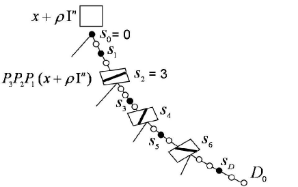
Figure 7: The choice of slabs at the nodes causes the phase tube to split at the nodes indexed by $I=\{2,4,6\}$. The nodes of depth $s_{k}$ for $k\not\in I$ are represented as black dots: $s_{0},s_{1},s_{3},s_{5},s_{7}$ ($D=7$). The other nodes in the paths are the white dots.

Lemma 6.4 allows us to eliminate the variables $x_{1},\ldots,x_{m}$: we premultiply $V_{|I}$ by the unit vector $u$ to find that

$$|\,\text{Aff}\,[\,y_{1},\ldots,y_{r}\,]+\delta\,|\leq(\varepsilon+\rho)N^{O(cm^{3}D)},$$ (25)

where the coefficients of the new affine form are bounded by $N^{O(cm^{3}D)}$. (We leave the constant $c$ in the exponent to highlight its influence.) The remarkable fact is that the variable $\delta$ is assured not to vanish during the elimination. Thus, as long as $\delta$ remains outside a gap of type $(\varepsilon+\rho)N^{O(cm^{3}D)}$, the phase tube formed by ${\mathbf{x}}+\rho\,{\mathbb{I}}^{n}$ and $P_{0},\ldots,P_{D}$ cannot split at every index of $I$. Counting the number of possible choices of slabs per node raises the number of gaps to $n^{O(|I|)}$. The argument assumes that $\delta$ has the same value in each of $|I|$ inequalities. It need not be so: each $\delta$ in (24) can be replaced by $\delta+\nu_{k}$ ($k\in I$), for $|\nu_{k}|\leq\rho$, and the new system of inequalities will still imply (25). A combinatorial argument shows how adding more gaps to the “exclusion zone” keeps branching low. Before proceeding with that final part of the proof, we summarize our results, using the bound $|\!\log\alpha|\geq\log e>1$.

Lemma 6.5

$\!\!\!.\,\,$ Let $N=n^{n^{2}/\gamma}$ and $\beta=1/(cm^{3}\log N)$, where $c$ is the constant of Lemma 6.4. Fix a path in ${\mathcal{T}}^{\,\mathbb{I}}_{m\,\rightarrow\,n-m}$ from the root and pick $D+1$ nodes on it of depth $0=s_{0}<\cdots<s_{D}$ satisfying (23); out of these nodes, choose a subset $I$ of size $\lceil D^{1-\beta^{m+1}}\rceil$. There exists an exclusion zone $W$ consisting of the union of at most $n^{O(|I|)}$ gaps of type $(\varepsilon+\rho)N^{O(cm^{3}D)}$, such that, for any interval $\Delta\subseteq{\mathbb{I}}\setminus W$ of length $\rho$ and any ${\mathbf{x}}\in{\mathbb{C}}[y_{1},\ldots,y_{r}]$, the phase tube formed by ${\mathbf{x}}+\rho\,{\mathbb{I}}^{n}$ cannot split at all the nodes of $I$ in ${\mathcal{T}}^{\Delta}_{m\,\rightarrow\,n-m}$ (assuming they exist).

The crux of the lemma is that it holds uniformly for all ${\mathbf{x}}$. To prove Lemma 6.3, we need to extend the previous lemma to all the paths of the coding tree of the prescribed length and remove from (23) the lower bound of $1/\gamma$ on the distance between consecutive splitting nodes. Fix $D_{0}\geq 2^{(1/\gamma)^{n+1}}$, and let $v$ be a node of ${\mathcal{T}}^{\,\mathbb{I}}_{m\,\rightarrow\,n-m}$ of depth $t_{v}=D_{0}$. Since the path is fixed, we can uniquely identify the node $v$ and its ancestors by their depths and denote by $P_{t}$ the transition matrix of the node at depth $t$. Define the node set $J=\{1/\gamma,2/\gamma,\ldots,D_{0}\}$, with $|J|=\lceil\gamma D_{0}\rceil$; recall that $1/\gamma=t_{c}$ is an integer. Let $K$ be the set of ancestors of $v$ at which the phase tube formed by ${\mathbf{x}}+\rho\,{\mathbb{I}}^{n}$ and $P_{0},\ldots,P_{D_{0}}$ splits (with respect to ${\mathcal{T}}^{\,\mathbb{I}}_{m\,\rightarrow\,n-m}$); assume that

$$|K|\geq D_{0}^{1-\gamma^{n+1}}.$$ (26)

We define $I$ to be the largest subset of $K$ with no two elements of $I\cup\{0\}$ at a distance less than $1/\gamma$; obviously, $|I|\geq\lfloor\gamma|K|\rfloor-1$. To define $s_{1},\ldots,s_{D}$, we add all of $J$ to $I$ (to keep distances between consecutive nodes small enough) and then clean up the set to avoid distances lower than allowed: we define $J^{\prime}$ to be the smallest subset of $J$ such that $L=I\cup(J\setminus J^{\prime})$ contains no two elements at a distance less than $1/\gamma$. Each element of $I$ can cause the disappearance of at most two elements in $J$ for the addition of one into $L$, hence $|J|/2\leq|L|\leq\gamma D_{0}+1$. By construction, consecutive elements of $L$ are at most $3/\gamma$ away from each other, so we can identify $L$ with the sequence $s_{1}<\cdots<s_{D}$. By $m<n$ and the specifications of $\gamma$ in Lemma 6.1 and $N,\beta$ in Lemma 6.5, we can verify that

$$\text{\rm(i)}\,\,\,D_{0}\geq 2^{(1/\gamma)^{n+1}}\geq\gamma^{-1}2^{(1/\beta)^{m+1}+1}\hskip 11.38092pt\text{and}\hskip 11.38092pt\text{\rm(ii)}\,\,\,D_{0}^{1-\gamma^{n+1}}\geq\hbox{$\frac{2}{\gamma}$}(\gamma D_{0}+1)^{1-\beta^{m+1}}.$$ (27)

Part (i) ensures (23). By Lemma 6.5, keeping $\delta$ outside the union $W$ of at most $n^{O(|I|)}$ gaps of type $(\varepsilon+\rho)N^{O(m^{3}D)}$ prevents $I$ from witnessing a phase tube split at each of its nodes, and hence keeps $K\supseteq I$ from being, as claimed, made entirely of “splitting” nodes. For this, we need to ensure that $|I|\geq D^{1-\beta^{m+1}}$, which follows from: (26); $|I|\geq\lfloor\gamma|K|\rfloor-1$; $D=|L|\leq\gamma D_{0}+1$; and part (ii) of (27).

We conclude that, as long as we choose an interval $\Delta\subseteq{\mathbb{I}}\setminus W$ of length $\rho$, the coding tree ${\mathcal{T}}^{\Delta}_{m\,\rightarrow\,n-m}$ cannot witness splits at all of the nodes of $K$ (if they exist—their existence is ensured only in ${\mathcal{T}}^{\,\mathbb{I}}_{m\,\rightarrow\,n-m}$) for the phase tube formed by any box ${\mathbf{x}}+\rho\,{\mathbb{I}}^{n}$, where $y_{1},\ldots,y_{r}$ are fixed and ${\mathbf{x}}\in{\mathbb{C}}[y_{1},\ldots,y_{r}]$. Note the order of the quantifiers: first, we fix the coordinates $y_{k}$ and the target length $D_{0}$, and we pick a large enough candidate splitting node set $K$ in ${\mathcal{T}}^{\,\mathbb{I}}_{m\,\rightarrow\,n-m}$; these choices determine the exclusion zone $W$; next, we pick a suitable $\Delta$ and then claim an impossibility result for any ${\mathbf{x}}$ in ${\mathbb{C}}[y_{1},\ldots,y_{r}]$. To complete the proof of Lemma 6.3, we bound, by $2^{D_{0}}$ and $n^{O(nD_{0})}$ respectively, the number of ways of choosing $K$ (hence $I$, $L$) and the number of nodes $v$ in ${\mathcal{T}}^{\,\mathbb{I}}_{m\,\rightarrow\,n-m}$ of depth $t_{v}=D_{0}$. $\Box$

Proof of Lemma 6.4.

We can make the assumption that $I$ includes $0$, since all cases easily reduce to it. Indeed, let $l$ be the smallest index in $I$. If $l>0$, subtract $l$ from the indices of $I$ to define $I^{\prime}\supseteq\{0\}$. Form the matrix $V^{\prime}_{|I^{\prime}}$ of vectors $v^{\prime}_{k}$, where $v_{k+l}=v^{\prime}_{k}A_{l}\cdots A_{0}$. Rewriting $V_{|I}$ as $V^{\prime}_{|I^{\prime}}A_{l}\cdots A_{0}$ takes us to the desired case: we (cosmetically) duplicate the last matrix, $P_{D}$, $l$ times to match the lemma’s assumptions and observe that, if $u^{T}V^{\prime}_{|I^{\prime}}={\mathbf{0}}$, then so does $u^{T}V_{|I}$. We may also assume that all $v_{k}$ are nonzero since the lemma is trivial otherwise. All the coordinates of $v_{k}$ can be expressed as $O(m^{2}(k+1)\log N)$-bit rationals sharing a common denominator; therefore,

$$N^{-O((k+1)m^{2})}\leq\|v_{k}\|_{1}\leq 2^{-k|\!\log\alpha|+O(\log n)}.$$ (28)

The affine hull of $V_{|I}$ is the flat defined by $\{\,z^{T}V_{|I}\,:\,z^{T}{\mathbf{1}}=1\,\}$: its dimension is called the affine rank of $V_{|I}$. Let $g(D,r)$ be the maximum value of $|I|$, for $\{0\}\subseteq I\subseteq\{0,\ldots,D\}$, such that $V_{|I}$ has affine rank at most $r$ and its affine hull does not contain the origin. Lemma 6.4 follows from this inequality, whose proof we postpone: for $r=0,\ldots,m-1$,

$$g(D,r)<D^{1-\beta^{m+1}}\,,\hskip 14.22636pt\text{for any}\,\,\,D\geq 2^{(1/\beta)^{m+1}},$$ (29)

where $\beta=|\!\log\alpha|/(cm^{3}\log N)$, for constant $c$ large enough. Indeed, given any $\{0\}\subseteq I\subseteq\{0,\ldots,D\}$ of size at least $D^{1-\beta^{m+1}}$, we have $|I|>g(D,m-1)$, so the affine hull of $V_{|I}$ contains the origin. If $r$ is its affine rank, then there exists $J\subseteq I$ of size $r+1$ such that the affine rank of $V_{|J}$ is $r$ and its affine hull contains the origin, hence coincides with the row space of $V_{|J}$, which is therefore of dimension $r$. This implies the existence of $r$ independent columns in $V_{|J}$ spanning its column space: add a column of $r+1$ ones to the right of them to form the $(r+1)$-by-$(r+1)$ matrix $M$. Since the affine hull of $V_{|J}$ contains the origin, there exists $z$ such that $z^{T}V_{|J}={\mathbf{0}}$ and $z^{T}{\mathbf{1}}=1$, which in turn shows that ${\mathbf{1}}_{r+1}$ lies outside the column space of $V_{|J}$; therefore $M$ is nonsingular. Since each one of its rows consists of $O(m^{2}D\log N)$-bit rationals with a common denominator,

$$|\!\det M|\geq N^{-O(m^{3}D)}.$$ (30)

Let $\xi$ be the $(r+1)$-dimensional vector whose $k$-th coordinate is the cofactor of the $k$-th entry in the last column of ones in $M$. Simple determinant cofactor expansions show that

$$\xi^{T}M=(\,\overset{r}{\overbrace{\,0,\ldots,0\,}},\det M).$$

Since the first $r$ columns of $M$ span the column space of $V_{|J}$, it follows that

$$\xi^{T}(\,V_{|J},{\mathbf{1}}_{r+1}\,)=(\,\overset{m}{\overbrace{\,0,\ldots,0\,}},\det M).$$

By Hadamard’s inequality, each coordinate of $\xi$ is at most $n^{O(m)}$ in absolute value, so straightforward rescaling and padding with zeroes turns $\xi$ into a suitable vector $u$ such that $u^{T}V_{|I}={\mathbf{0}}$ and $u^{T}{\mathbf{1}}\geq N^{-c_{1}m^{3}D}$, for an absolute constant $c_{1}$ that does not depend on $c$. Replacing $c$ by $\max\{c,c_{1}\}$ establishes Lemma 6.4.

It suffices now to prove (29), which we do by induction on $r$. If $V_{|I}$ has affine rank $r=0$ and its affine hull does not contain the origin, then all the rows of $V_{|I}$ are equal and nonzero. Since $V_{|I}$ has the row $v_{0}$, it follows from (28) that $|I|\leq 1+\max\{k\in I\}=O(|\!\log\alpha|^{-1}m^{2}\log N)$, hence

$$g(D,0)\leq\beta^{-1}.$$ (31)

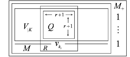
Figure 8: Why a large value of $k_{i}$ implies that the affine hull of $V_{|I}$, hence of $M$, contains the origin.

Assume now that $r>0$ and that $V_{|I}$ has affine rank exactly $r$. Put $I=\{k_{0},k_{1},\ldots,k_{i}\}$, with $k_{0}=0$, and consider the smallest $j$ such that $V_{|J}$ has affine rank $r$, where $J=\{k_{0},k_{1},\ldots,k_{j}\}\subseteq I$. Since the origin is not in the affine hull of $V_{|I}$ hence of $V_{|J}$, we can always pick a subset $K\subseteq J$ consisting of $r+1$ independent rows: let $M=V_{|K\cup\{k_{i}\}}$ denote the $(r+2)$-by-$m$ matrix formed by adding the row $v_{k_{i}}$ at the bottom of $V_{|K}$. Since $V_{|I}$ has affine rank $r$, its rank is $r+1$ (using once again the noninclusion of $O$ in the affine hull of $V_{|I}$), hence so is the rank of $M$. We show that if $k_{i}$ is large enough, the system below is feasible in $\xi\in{\mathbb{R}}^{r+2}$:

$$\xi^{T}M_{+}=(\,\overset{m}{\overbrace{\,0,\ldots,0\,}},1),$$ (32)

where $M_{+}$ is the $(r+2)$-by-$(m+1)$ matrix $(M,{\mathbf{1}}_{r+2})$, which leads to a contradiction. This is the crux of the argument and makes essential use of the rapid decay of the vectors $v_{k}$. Assume that $k_{i}>ck_{j}|\!\log\alpha|^{-1}m^{3}\log N$, for a large enough constant $c$. We first show that $M_{+}$ is of rank $r+2$. Pick $r+1$ independent columns of $V_{|K}$, which is possible since the latter has rank $r+1$, to form the full-ranked $(r+1)$-by-$(r+1)$ matrix $Q$. Add a new row to it by fitting the relevant part of $v_{k_{i}}$ (the last row of $M$) and call $R$ the resulting $(r+2)$-by-$(r+1)$ matrix (Fig. 8); consistent with our notation, $R_{+}$ will denote the matrix $(R,{\mathbf{1}})$. A cofactor expansion of the determinant of $R_{+}$ along the bottom row shows that

$$|\!\det R_{+}|\geq|\!\det Q|-\Delta\|v_{k_{i}}\|_{1},$$

where $\Delta$ is an upper bound on the absolute values of the cofactors other than $\det Q$. In view of (28), the matrix entries involved in these cofactors are all in $n^{O(1)}$; by Hadamard’s inequality, this shows that we can set $\Delta=n^{O(m)}$. Likewise, we find that

$$\|v_{k_{i}}\|_{1}\leq 2^{-k_{i}|\!\log\alpha|+O(\log n)}.$$

Since $Q$ is nonsingular, we can adapt (30) to derive $|\!\det Q|\geq N^{-O(m^{3}k_{j})}$, hence $|\!\det R_{+}|>0$. It follows that the linear system (32) is feasible if we replace $M_{+}$ by $R_{+}$. As it happens, there is no need to do so since every column of $M$ missing from $R$ lies in the column space of the latter: thus the missing homogeneous equalities are automatically satisfied by the solution $\xi$. The feasibility of (32) contradicts our assumption that the origin is outside the affine hull of $V_{|I}$; therefore

$$k_{j}\geq\beta k_{i}>0,$$ (33)

where $\beta=|\!\log\alpha|/(cm^{3}\log N)$. The affine rank of $V_{|\{k_{0},\ldots,k_{j-1}\}}$ is $r-1$ and its affine hull does not contain the origin, so $j\leq g(k_{j-1},r-1)$, with $g(0,r-1)=1$. Let $w_{0}=a_{k_{j}}$ and, for $k>0$, $w_{k}=a_{k_{j}+k}A_{k_{j}+k}\cdots A_{k_{j}+1}$, thus ensuring that $v_{k_{j}+k}=w_{k}A_{k_{j}}\cdots A_{0}$. Since the affine hull of $V_{|I}$ does not contain the origin, neither does that of the matrix $W$ with rows $w_{0},w_{k_{j+1}-k_{j}},\ldots,w_{k_{i}-k_{j}}$. It follows that the affine rank of $W$ is less than $m$, so $i-j+1\leq g(k_{i}-k_{j},m-1)$, hence $i\leq g(k_{j-1},r-1)+g(k_{i}-k_{j},m-1)-1$. By (33) and $i=|I|-1$, we derive, by monotonicity,

$$|I|\leq g(k,r-1)+g(D-k,m-1),$$

where $\beta D\leq k\leq D$; hence, by (31), for $m>0$ and $D\geq 0$:

$$g(D,r)\leq\begin{cases}\,1&\text{ if $D=0$ }\\ \,\beta^{-1}&\text{ if $r=0$}\\ \,g(n_{1},m-1)+\cdots+g(n_{r},m-1)+\beta^{-1}&\text{ if $0<r<m$,}\end{cases}$$

where $n_{1}+\cdots+n_{r}\leq(1-\beta^{s})D$, with $s=|\{\,i\,|\,n_{i}>0\,\}|$. Setting $\eta=\beta^{m}$, we check that, for all $D>0$ and $m>0$,

$$g(D,m-1)\leq\beta^{-2}(2D^{1-\eta}-1).$$ (34)

The case $m=1$ follows from $g(D,0)\leq\beta^{-1}$. For $m>1$, we begin with the case $s=0$, where

$$g(D,m-1)\leq m-1+\beta^{-1}\leq\beta^{-2}(2D^{1-\eta}-1).$$

This follows from $\alpha\geq N^{-O(1)}$, which implies that $\beta m^{3}$ can be made arbitrarily small by increasing $c$. For $s=1$,

$$\begin{split}g(D,m-1)&\leq\beta^{-2}(2(1-\beta)^{1-\eta}D^{1-\eta}-1)+m-2+\beta^{-1}\\ &\leq 2\beta^{-2}D^{1-\eta}-(2\beta^{-1}(1-\eta)-O(1))D^{1-\eta}-\beta^{-2}+\beta^{-1}+m-2\\ &\leq\beta^{-2}(2D^{1-\eta}-1).\end{split}$$

Assume that $s>1$. Being concave, the function $x\mapsto x^{1-\eta}$ is subadditive for $x\geq 0$; therefore,

$$n_{1}^{1-\eta}+\cdots+n_{r}^{1-\eta}\leq(1-\beta^{s})^{1-\eta}D^{1-\eta}.$$

Setting $r=m-1$, relation (34) follows from the inequality,

$$\begin{split}g(D,m-1)&\leq\beta^{-2}(2(1-\beta^{s})^{1-\eta}D^{1-\eta}-s)+m-s-1+\beta^{-1}\\ &\leq 2\beta^{-2}(1-\beta^{m-1})^{1-\eta}D^{1-\eta}-\hbox{$\frac{3}{2}$}\beta^{-2}\leq 2\beta^{-2}D^{1-\eta}-\beta^{-2},\end{split}$$

which proves (34), hence (29) and Lemma 6.4. $\Box$

6.3 The degree structure

We decompose the global coding tree into three layers: the top one has no degree constraints; the second has mean degree less than two; and the third has no branching. Consider a placement of the $B$-agents, such that the diameter of each $B_{i}$ is less than $n^{-bn}$. By the agreement rule, the communication subgraph induced by the $B$-agents is frozen and its transition matrix $Q$ is fixed and independent of the particular placement of the $B$-agents. By Perron-Frobenius, or simply by repeating the proof of Lemma 6.1, we derive the existence of a rank-$r$ stochastic matrix

$${\widetilde{Q}}=\text{\rm diag}\,({\mathbf{1}}_{n_{1}}\chi_{1}^{T},\ldots,{\mathbf{1}}_{n_{r}}\chi_{r}^{T})$$

such that $\chi_{i}\in{\mathbf{R}}^{n_{i}}$ and $\|Q^{k}-{\widetilde{Q}}\|_{\text{\rm max}}\leq e^{-kn^{-O(n)}}$. The $B$-agents find themselves attracted to the fixed point ${\mathbf{y}}={\widetilde{Q}}\xi$, where $\xi\in{\mathbb{R}}^{n-m}$ is their initial state vector and

$${\mathbf{y}}=(\,\overset{n_{1}}{\overbrace{y_{1},\ldots,y_{1}}},\ldots,\overset{n_{r}}{\overbrace{y_{r},\ldots,y_{r}}}\,).$$

Define $\Upsilon=\Omega^{m}\times(\Omega^{n-m}\cap\Upsilon_{B})$, where

$$\Upsilon_{B}={\mathbf{y}}+(n^{-2bn}\,{\mathbb{I}}^{n-m})\cap\ker{\widetilde{Q}}.$$

If ${\mathbf{x}}\in\Upsilon$, the diameter of any group $B_{i}$ is at most $2n^{-2bn}<n^{-bn}$ so the communication graph induced by their agents is frozen and remains so. The $B$-agents are attracted to ${\mathbf{y}}$. This follows easily, as does the next lemma, whose proof we omit, from the stochasticity of $Q$ and the identities: ${\widetilde{Q}}Q=Q{\widetilde{Q}}={\widetilde{Q}}^{2}={\widetilde{Q}}$.

Lemma 6.6

$\!\!\!.\,\,$ The set $\Upsilon$ is forward-invariant. Furthermore, any $\xi\in{\mathbf{y}}+n^{-2bn}\,{\mathbb{I}}^{n-m}$ belongs to $\Upsilon_{B}$ if and only if ${\widetilde{Q}}\xi={\mathbf{y}}$.

We set $\varepsilon,\rho,D_{0}$ as in Lemma 6.3 and call an interval $\Delta$ free if it does not intersect the exclusion zone $W=W({\mathbf{y}})$. As usual, we choose the perturbation sample space $n^{-b}\,{\mathbb{I}}$ to make perturbations inconsequential in practice. For counting purposes, it is convenient to partition $n^{-b}\,{\mathbb{I}}$ into canonical intervals of length $\rho$ (with possibly a single smaller one). A gap of $W$ can keep only $(1+\varepsilon/\rho)n^{O(n^{5}D_{0})}$ canonical intervals from being free, so the Lebesgue measure of the free ones satisfies:

$$\text{Leb}\,\Bigl{\{}\,\bigcup\,\text{free canonical intervals}\,\Bigr{\}}\,\geq 2n^{-b}-(\varepsilon+\rho)n^{O(n^{5}D_{0})}.$$ (35)

Fixing the $B$-agent attractor.

With ${\mathbf{y}}$ fixed, we pick a free canonical interval $\Delta$ and focus on the global coding tree ${\mathcal{T}}^{\Delta|\Upsilon}_{m\,\rightarrow\,n-m}$, with the superscripts indicating the perturbation and phase spaces, respectively. For any node $v$ of depth $t_{v}\geq t_{c}$, the limit matrix $D_{u}$ in Lemma 6.2 is the same for all nodes $u$ of depth $t_{c}$. Indeed,

$$\Bigl{\|}\,P_{\leq v}-\begin{pmatrix}0&C_{v}\\ 0&{\widetilde{Q}}\end{pmatrix}\,\Bigr{\|}_{\text{max}}\leq e^{-\gamma t_{v}}.$$

Pick $v$ of depth $t_{v}\geq 3t_{c}$ and let $w$ be its ancestor at depth $t_{w}=\lfloor t_{v}/2\rfloor$. Given ${\mathbf{x}}\in U_{v}\subseteq\Upsilon$,

$$\begin{split}{\mathbf{x}}^{\prime}&=f^{t_{w}}({\mathbf{x}})=P_{\leq w}\,{\mathbf{x}}\in\begin{pmatrix}C_{w}\\ {\widetilde{Q}}\end{pmatrix}(x_{m+1},\ldots,x_{n})^{T}+ne^{-\gamma t_{w}}\,{\mathbb{I}}^{n}\\ &\in\begin{pmatrix}C_{w}(x_{m+1},\ldots,x_{n})^{T}\\ {\mathbf{y}}\end{pmatrix}+ne^{-\gamma t_{w}}\,{\mathbb{I}}^{n}.\end{split}$$

By Lemma 6.6, ${\mathbf{x}}^{\prime}\in\Upsilon$, so there exists a node $v^{\prime}$ of depth $t_{v^{\prime}}=t_{v}-t_{w}\geq t_{c}$ such that,

$$f^{t_{v}}({\mathbf{x}})=f^{t_{v^{\prime}}}({\mathbf{x}}^{\prime})=P_{\leq v^{\prime}}\,{\mathbf{x}}^{\prime}\in\begin{pmatrix}C_{v^{\prime}}\\ {\widetilde{Q}}\end{pmatrix}({\mathbf{y}}+ne^{-\gamma t_{w}}\,{\mathbb{I}}^{n})+ne^{-\gamma t_{v^{\prime}}}\,{\mathbb{I}}^{n}\subseteq\begin{pmatrix}C_{v^{\prime}}{\mathbf{y}}\\ {\mathbf{y}}\end{pmatrix}+2ne^{-\gamma t_{v}/3}\,{\mathbb{I}}^{n}.$$

It is important to note that $v^{\prime}$ depends only on $v$ and not on ${\mathbf{x}}\in U_{v}$: indeed, the phase tube from $U_{v}$ between time $t_{w}$ and $t_{v}$ does not split; therefore $f^{t_{w}}(U_{v})\subseteq U_{v^{\prime}}$. It follows that, for $t_{v}\geq 3t_{c}$ and $v^{\prime}=v^{\prime}(v)$,

$$V_{v}\subseteq\begin{pmatrix}C_{v^{\prime}}{\mathbf{y}}\\ {\mathbf{y}}\end{pmatrix}+2ne^{-\gamma t_{v}/3}\,{\mathbb{I}}^{n}.$$ (36)

The $A$-agents evolve toward convex combinations of the $B$-agents, which themselves become static. The weights of these combinations (ie, the barycentric coordinates of the $A$-agents), however, might change at every node, so there is no assurance that the orbit is always attracted to a limit cycle. The layer decomposition of the coding tree, which we describe next, allows us to bound the nesting time while exhibiting weak yet sufficient conditions for periodicity.

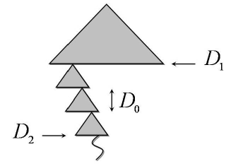
Figure 9: The global coding tree is stratified into three layers, with decreasing branching rates.

To stratify the coding tree ${\mathcal{T}}^{\Delta|\Upsilon}_{m\,\rightarrow\,n-m}$ into layers, we set up three parameters $D_{0}$, $D_{1}$, and $D_{2}$: the first targets the topological entropy; the second specifies the height of the first layer; the third indicates the nesting time. We examine each one in turn and indicate their purposes and requirements.

First layer.

By (36), the phase tubes get thinner over time at a rate of roughly $e^{-\gamma/3}$, while the tree is branching at a rate of $n^{O(n)}$. To ensure that the topological entropy is zero, the product of these two rates should be less than 1: with $\gamma<1$, this is far from being the case, so we need a sparsification mechanism. This is where Lemma 6.3 comes in. Indeed, deep enough in ${\mathcal{T}}^{\Delta|\Upsilon}_{m\,\rightarrow\,n-m}$, the size of a subtree of height $D_{0}$ is at most

$$D_{0}(n^{O(n)})^{D_{0}^{1-\gamma^{n+1}}},$$

while the tubes get thinner at a rate of $2ne^{-\gamma D_{0}/3}$ for every consecutive $D_{0}$ nodes: the choice of $D_{0}$ below ensures that the product is less than 1, as desired. We justify this choice formally below.

$$\hskip 28.45274ptD_{0}\geq 2^{(1/\gamma)^{n+2}} D_{0}$$ [ big enough for thinning to outpace branching ]. (37)

Second layer.

Technically, Lemma 6.3 addresses only the branching of the phase tube formed by a small box ${\mathbf{x}}+\rho\,{\mathbb{I}}^{n}$, for ${\mathbf{x}}\in{\mathbb{C}}[y_{1},\ldots,y_{r}]$, whereas we are concerned here with phase tubes originating at some cell $V_{v}$ of ${\mathcal{T}}^{\Delta|\Upsilon}_{m\,\rightarrow\,n-m}$. To make $V_{v}$ thin enough, we choose a node $v$ deep in the tree. By (36), $V_{v}\subseteq{\mathbf{x}}+\rho\,{\mathbb{I}}^{n}$, for ${\mathbf{x}}\in{\mathbb{C}}[y_{1},\ldots,y_{r}]$, provided that $t_{v}\geq D_{1}$ and

$$\hskip 28.45274ptD_{1}\geq\frac{3}{\gamma}\log\frac{2n}{\rho} D_{1} \rho$$ [ big enough for tree branches to be thinner than ]. (38)

Note that the requirement in (36) that $t_{v}\geq 3t_{c}=3/\gamma$ is implied by $t_{v}\geq D_{1}$. In view of Lemma 6.3, the number of nodes in ${\mathcal{T}}^{\Delta|\Upsilon}_{m\,\rightarrow\,n-m}$ of depth no greater than $t\geq D_{1}$, is bounded by

$$\underset{{\tt depth\,\,D_{1}}}{\underbrace{\,n^{O(nD_{1})}\,}}\times\underset{{\tt from\,\,D_{1}\,\,to\,\,t\,\,in\,\,chunks\,\,of\,\,D_{0}}}{\underbrace{\,n^{O(nD_{0}^{1-\gamma^{n+1}}\lfloor(t-D_{1})/D_{0}\rfloor)}\,}}\times\underset{{\tt truncated\,\,chunk}}{\underbrace{\,n^{O(nD_{0})}\,}}\times\underset{{\tt single\,\,paths}}{\underbrace{\,D_{0}\,}};$$

hence, for any $t\geq D_{1}$,

$$\Bigl{|}\,\{\,v\in{\mathcal{T}}^{\Delta|\Upsilon}_{m\,\rightarrow\,n-m}\,|\,t_{v}\leq t\,\}\,\Bigr{|}\leq n^{O(nD_{0}+nD_{1}+ntD_{0}^{-\gamma^{n+1}})}\,.$$ (39)

Third layer.

The bottom layer of the stratified global coding tree begins at a depth $D_{2}\geq D_{0}+D_{1}$. If the node $v$ of depth $t_{v}\geq D_{2}$ has nontrivial branching, then, by continuity, $V_{v}$ contains a point right on the boundary of the global margin. By (36), this implies the existence of $\zeta\in{\mathbb{R}}^{n}$ such that $\|\zeta\|_{\infty}\leq 2ne^{-\gamma\,D_{2}/3}$ and $\text{Aff}\,[{\mathbf{y}}+\zeta]=\delta$, where the coefficients of the affine form are of magnitude $n^{O(1)}$ and depend only on the node $v$. It then follows from (39) that ${\mathcal{T}}^{\Delta^{\prime}|\Upsilon}_{m\,\rightarrow\,n-m}$ has no nontrivial branching at depth $D_{2}$, provided that $\Delta^{\prime}=\Delta\setminus W^{\prime}$, where $W^{\prime}$ consists of gaps of type $n^{O(1)}e^{-\gamma\,D_{2}/3}$ numbering at most

$$\underset{{\tt\#\,nodes\,\,at\,\,depth\,\,D_{2}}}{\underbrace{\,n^{O(nD_{0}+nD_{1}+nD_{2}D_{0}^{-\gamma^{n+1}})}\,}}\times\underset{{\tt\#\,margin\,\,slabs}}{\underbrace{\,n^{O(1)}\,}}.$$

This calculation, in which $\varepsilon$ played no role, puts a bound of $D_{2}$ on the nesting time. It follows that

$$\text{Leb}\,(W^{\prime})\leq e^{-\gamma\,D_{2}/3}n^{O(nD_{0}+nD_{1}+nD_{2}D_{0}^{-\gamma^{n+1}})}$$ (40)

Pick an arbitrarily small $\varepsilon_{o}>0$ and a large enough constant $d=d(b,c)$; recall that $\gamma=n^{-cnt_{o}}$. We set the parameters $\rho=\varepsilon_{o}^{2}\,n^{-dn^{5}D_{0}}$ and $\varepsilon\leq\min\,\{\,\rho,e^{-\gamma D_{2}\,}\}$, where, rounding up to the nearest integer,

$$\begin{cases}\,D_{0}=\,2^{d(1/\gamma)^{n+2}}\\ \,D_{1}=\,\frac{d^{2}}{\gamma}(n^{6}D_{0}+|\!\log\varepsilon_{o}|)\\ \,D_{2}=\,\frac{d}{\gamma}(n^{2}D_{1}+|\!\log\varepsilon_{o}|).\end{cases}$$ (41)

We verify that conditions (37, 38) are both satisfied and that

$$D_{1}\geq D_{2}D_{0}^{-\gamma^{n+1}}.$$ (42)

Thus the measure bound (40) implies that $\text{Leb}\,(W^{\prime})\leq\rho 2^{-D_{0}}$. By making $\varepsilon$ tend to $0$, the point ${\mathbf{x}}$ vanishes with arbitrarily small probability for random $\delta\in\Delta^{\prime}$. By Lemma 4.4, this implies that, with probability at least $1-2^{-D_{0}}$, subjecting the system’s margin to a perturbation $\delta$ chosen randomly in $\Delta$ makes the orbit of any ${\mathbf{x}}\in\Upsilon$ attracted to a limit cycle (or a switching leaf): we call this success. The sum of the period and preperiod is bounded by the number of nodes of depth at most $D_{2}$ (the nesting time), which, by (39, 42), is no greater, conservatively, than

$$\bar{p}=n^{O(nD_{1})}\leq(1/\varepsilon_{o})^{O(\gamma^{-2})}\,2^{D_{0}\gamma^{-1}n^{O(1)}}.$$ (43)

We bound the attraction rate by appealing to Lemmas 4.5 and 6.2. Note that if $p$ is the period then so is $p\lceil(\log 2n)/\gamma\rceil$. This choice of $p$ still satisfies the upper bound (43) while ensuring that, at every period, the error bound in Lemma 6.2 is at most $\frac{1}{2n}$. The row-sums in $A$ in Lemma 4.5 are at most $1/2$, so we can set $\mu=e^{-\gamma}$. Since $\nu\leq D_{2}$ and $(\#{\mathcal{S}}_{\nu})\lceil(\log 2n)/\gamma\rceil\leq\bar{p}$, it follows that

$$\theta_{\alpha}\leq D_{0}^{O(D_{0})}(1/\varepsilon_{o})^{O(\gamma^{-2})}\log\hbox{$\frac{1}{\alpha}$},$$ (44)

for any $0<\alpha<1/2$. The perturbation space is not $\Delta$ but $n^{-b}\,{\mathbb{I}}$, so we apply the previous result to each free canonical interval and argue as follows. If $\Lambda$ is the measure of the union of all the free canonical intervals, then the perturbations that do not guarantee success have measure at most $(2n^{-b}-\Lambda)+2^{-D_{0}}\Lambda$. Dividing by $2n^{-b}$ and applying (35) shows that

$$\text{Prob}\,[\,\text{failure in}\,\,{\mathcal{T}}^{\,n^{-b}\,\mathbb{I}\,|\,\Upsilon}_{m\,\rightarrow\,n-m}\,]\leq 1-(1-2^{-D_{0}})(\,1-(\varepsilon+\rho)n^{O(n^{5}D_{0})}\,)\leq 2^{1-D_{0}}.$$ (45)

The nesting time is at most $D_{2}$, which, by (39, 42), implies that

$$h({\mathcal{T}}^{\,n^{-b}\,\mathbb{I}\,|\,\Upsilon}_{m\,\rightarrow\,n-m})\leq O(D_{1}n\log n)\leq\hbox{$\frac{1}{\gamma}$}(D_{0}+|\!\log\varepsilon_{o}|)n^{O(1)}.$$ (46)

Freeing the $B$-agents.

Set $D_{3}=\lceil 3bt_{c}n\log n\rceil$ and fix ${\mathbf{x}}$ in $\Omega^{n}$. Let $\xi$ denote the projection of $f^{D_{3}}({\mathbf{x}})$ onto the last $n-m$ coordinate axes. By Lemma 6.2 and $t_{c}=1/\gamma$ (Lemma 6.1), the coding tree ${\mathcal{T}}^{\,n^{-b}\,\mathbb{I}}_{m\,\rightarrow\,n-m}$ has $n^{O(nt_{c})}$ nodes $u$ such that $t_{u}=t_{c}$ and

$$\xi\in{\mathbf{y}}+ne^{-\gamma D_{3}}\,{\mathbb{I}}^{n-m}\subseteq{\mathbf{y}}+n^{-2bn}\,{\mathbb{I}}^{n-m},$$

where ${\mathbf{y}}=D_{u}(x_{m+1},\ldots,x_{n})^{T}$. The state vector for the $B$-agents is $\xi$ at time $D_{3}$ and $Q^{t-D_{3}}\xi$ at $t>D_{3}$, where $Q$ is the transition matrix of the frozen communication subgraph joining the $B$-agents at time $D_{3}$. By taking $t$ to infinity, it follows that ${\mathbf{y}}={\widetilde{Q}}\xi$ and, by Lemma 6.6, $\xi\in\Upsilon_{B}$ hence $f^{D_{3}}({\mathbf{x}})\in\Upsilon$. We can then apply the previous result. Since ${\mathbf{x}}$ is fixed, only the choice of random perturbation $\delta$ can change which path in ${\mathcal{T}}^{\,n^{-b}\,\mathbb{I}}_{m\,\rightarrow\,n-m}$ the orbit will follow. The failure probability of (45) needs to be multiplied by the number of nodes $u$, which yields an upper bound of $n^{O(nt_{c})}2^{1-D_{0}}$; hence

$$\text{Prob}\,[\,\text{failure in}\,\,{\mathcal{T}}^{\,n^{-b}\,\mathbb{I}}_{m\,\rightarrow\,n-m}\,]\leq 2^{-D_{0}/2}.$$ (47)

If ${\mathcal{T}}^{*}$ denotes the part of the global coding tree extending to depth $D_{3}$, then

$${\mathcal{T}}^{\,n^{-b}\,\mathbb{I}}_{m\,\rightarrow\,n-m}={\mathcal{T}}^{*}\,\otimes\,{\mathcal{T}}^{\,n^{-b}\,\mathbb{I}\,|\,\Upsilon}_{m\,\rightarrow\,n-m}.$$

The tree ${\mathcal{T}}^{*}$ has at most $n^{O(nt_{c})}D_{3}$ nodes; therefore, by (46),

$$h({\mathcal{T}}^{\,n^{-b}\,\mathbb{I}}_{m\,\rightarrow\,n-m})\leq O(t_{c}n\log n+\log D_{3})+h({\mathcal{T}}^{\,n^{-b}\,\mathbb{I}\,|\,\Upsilon}_{m\,\rightarrow\,n-m})\leq\hbox{$\frac{1}{\gamma}$}(D_{0}+|\!\log\varepsilon_{o}|)n^{O(1)}.$$ (48)

6.4 Removing persistence

We use direct products to relax the condition that the permanent graph $H$ be fixed once and for all. This touches on the non-Markovian nature of the system, a feature we chose to ignore in the previous section. We explain now why this was legitimate. Because the switching condition is about time differences and not absolute times, any subpath in the coding tree has an incarnation as a path from the root. Equivalently, any interval of a trajectory appears as the prefix of another trajectory. This property explains why, following (23), we could argue that $A_{k}$ was of the form $A_{\leq w}$. Likewise, in the derivations leading to (36), we used the fact that $f^{t_{v}}({\mathbf{x}})=f^{t_{v}-t_{w}}(f^{t_{w}}({\mathbf{x}}))$, an identity that might not always hold in a non-Markovian setting, but which, in this case, did. Finally, weren’t we too quick to appeal to Lemma 4.4 for periodicity since its proof relied heavily on the Markov property? To see why the answer is no, observe that the argument did establish the periodicity of the “wrap-around” system derived from ${\mathcal{T}}^{\Delta^{\prime}|\Upsilon}_{m\,\rightarrow\,n-m}$ by redirecting any trajectory that reaches the nesting depth to the root. The only problem is that this system, being Markovian, is not the one modeled by the coding tree. Wrapping around resets the time to zero, which might cause switching conditions to be missed and trajectories to be continued when they should be stopped: none of this stops nonvanishing orbits from being periodic, however.

We now show how to relax the permanent graph assumption. The idea is to begin with $H$ set as the complete graph and update it at each switching leaf by removing the edge(s) whose missing presence causes the node to be a switching leaf. We then append to each such leaf the coding tree, suitably cropped, defined with respect to the new value of $H$. We model this iteration by means of direct products, using $m_{k}$ to denote the number of $A$-agents in the block-directional system used in the $k$-th product:

$${\mathcal{T}}^{\,n^{-b}\,\mathbb{I}}_{n}\,\Longrightarrow\,\,\bigotimes_{k=1}^{k_{0}}\,{\mathcal{T}}^{\,n^{-b}\,\mathbb{I}}_{m_{k}\,\rightarrow\,n-m_{k}}.$$ (49)

The upper limit $k_{0}$ is bounded by $n(n-1)$; note that each decision procedure ${\mathcal{G}}_{ij}$ needs it own counter. To keep the failure probability small throughout the switching of dynamics, we need to update the value of $D_{0}$ in (41) at each iteration, so we define $C_{k}$ as its suitable value for a persistent graph consisting of $k$ (nonloop) directed edges and let $\phi_{k}$ denote the maximum failure probability for such a graph: $C_{n(n-1)}\geq D_{0}$ and $\phi_{0}=0$. The logarithm of the number of switching leaves is at most the word-entropy; by (47, 48), for $k>0$,

$$\phi_{k}\leq 2^{-C_{k}/2}+2^{\gamma^{-1}(C_{k}+|\!\log\varepsilon_{o}|)n^{a}}\phi_{k-1},$$

for some constant $a>0$. Setting

$$C_{n(n-1)-j}=\lceil\gamma^{-j}n^{2aj}(D_{0}+3|\!\log\varepsilon_{o}|)\rceil,$$

for $j=0,\ldots,n(n-1)$, we verify by induction that $\phi_{k}\leq 2^{1-C_{k}/2}$, for $k=0,\ldots,n(n-1)$; hence,

$$\text{Prob}\,[\,\text{failure in nonpersistent}\,\,{\mathcal{T}}^{\,n^{-b}\,\mathbb{I}}_{m\,\rightarrow\,n-m}\,]\leq\phi_{n(n-1)}\leq 2^{1-\frac{1}{2}(D_{0}+3|\!\log\varepsilon_{o}|)}\leq\varepsilon_{o}.$$

The attraction rate is still exponential: using (44) yields a geometric series summing up to

$$\theta_{\alpha}\leq C_{0}^{O(C_{0})}(1/\varepsilon_{o})^{O(\gamma^{-2})}\log\hbox{$\frac{1}{\alpha}$}\leq O_{n,\varepsilon_{o},t_{o}}(\log\hbox{$\frac{1}{\alpha}$}),$$ (50)

for any $0<\alpha<1/2$. By (43), the period and preperiod are bounded by

$$(1/\varepsilon_{o})^{O(\gamma^{-2})}\,2^{C_{0}\gamma^{-1}n^{O(1)}}\leq(1/\varepsilon_{o})^{O_{n,\varepsilon_{o},t_{o}}(1)},$$

which completes the proof of Theorem 1.1. $\Box$

Acknowledgments

I wish to thank Pascal Koiran and John Tsitsiklis for helpful conversations.

References

- [1]
- [2] Acemoglu, D., Dahleh, M.A., Lobel, I., Ozdaglar, A. Bayesian learning in social networks, LIDS report 2780, 2009.
- [3] Alur, R., Henzinger, T.A., Sontag, E.D. Hybrid Systems III. Verification and Control, Springer Verlag, Berlin, LNCS 1066, 1996.
- [4] Ballerini, M., Cabibbo, N., Candelier, R., Cavagna, A., Cisbani, E., Giardina, I., Lecomte, V., Orlandi, A., Parisi, G., Procaccini, A., Viale, M., Zdravkovic, V. Interaction ruling animal collective behavior depends on topological rather than metric distance: Evidence from a field study, Proc. National Academy of Sciences 105 (2008), 1232-1237.
- [5] Blondel, V.D., Hendrickx, J.M., Olshevsky, A., Tsitsiklis, J.N. Convergence in multiagent coordination, consensus, and flocking, Proc. 44th IEEE Conference on Decision and Control, Seville, Spain, 2005.
- [6] Blondel, V.D., Hendrickx, J.M., Tsitsiklis, J.N. On the 2R conjecture for multi-agent systems, Proc. European Control Conference 2007 (ECC 2007), July 2007, 874-881, Kos (Greece), 2007.
- [7] Blondel, V.D., Hendrickx, J.M., Tsitsiklis, J.N. On Krause’s multi-agent consensus model with state-dependent connectivity, IEEE Transactions on Automatic Control 54, 11 (2009), 2586–2597.
- [8] Blondel, V.D., Tsitsiklis, J.N. A survey of computational complexity results in systems and control, Automatica 36 (2000), 1249–1274.
- [9] Braverman, M., Grigo, A., Rojas, C. Noise vs computational intractability in dynamics, Proc. 3rd ITCS (2012), 128–141.
- [10] Bruin, H., Deane, J.H.B. Piecewise contractions are asymptotically periodic, Proc. American Mathematical Society 137, 4 (2009), 1389–1395.
- [11] Bullo, F., Cortés, J., Martinez, S., Distributed Control of Robotic Networks, Applied Mathematics Series, Princeton University Press, 2009.
- [12] Buzzi, J. Piecewise isometries have zero topological entropy , Ergod. Theory Dyn. Syst. 21 (2001), 1371 1377. MR1855837 (2002f:37029)
- [13] Cao, M., Spielman, D.A. Morse, A.S. A lower bound on convergence of a distributed network consensus algorithm, 44th IEEE Conference on Decision and Control, and the European Control Conference 2005, Seville, Spain, 2005
- [14] Castellano, C., Fortunato, S., Loreto, V. Statistical physics of social dynamics, Rev. Mod. Phys. 81 (2009), 591–646.
- [15] Catsigeras, E., Budelli, R. Topological dynamics of generic piecewise continuous contractive maps in dimensions, International Journal of Pure and Applied Mathematics, 68 (2011), 61 -83.
- [16] Cessac, B. A discrete time neural network model with spiking neurons: rigorous results on the spontaneous dynamics, J. Math. Biol. 56 (2008), 311 -345.
- [17] Chazelle, B. The convergence of bird flocking, arXiv:0905.4241v1, 2009. Prelim. version in ACM SoCG 2010.
- [18] Chazelle, B. The total -energy of a multiagent system, SIAM J. Control Optim. 49 (2011), 1680–1706.
- [19] Collins, G. E. Quantifier elimination for real closed fields by cylindrical algebraic decomposition, Proc. 2nd GI Conf. Automata Theory and Formal Languages, New York, Springer-Verlag (1975), 134–183.
- [20] Condon, A., Lipton, R.J. On the complexity of space bounded interactive proofs, Proc. 30th IEEE Symp. on Foundations of Computer Science (1989), 462–267.
- [21] Conradt, L., Roper, T.J. Group decision making in animals, Nature 421 (2003), 155–158.
- [22] Cucker, F., Smale, S. Emergent behavior in flocks, IEEE Trans. Automatic Control 52 (2007), 852–862.
- [23] Devaney, R.L. An Introduction to Chaotic Dynamical Systems, 2nd edition, Westview Press, 2003.
- [24] Dittmer, J.C. Consensus formation under bounded confidence, Nonlinear Analysis, Theory, Methods & Applications, 47 (2001), 4615–4622.
- [25] Earl, M.G., Strogatz, S.H. Synchronization in oscillator networks with delayed coupling: a stability criterion, Phys. Rev. E, 67 (2003), 036204(1–4).
- [26] Gazi, V., Passino, K.M. Stability analysis of swarms, IEEE Transactions on Automatic Control 48 (2003), 692–697.
- [27] Hegselmann, R., Krause, U. Opinion dynamics and bounded confidence models, analysis, and simulation, J. Artificial Societies and Social Simulation 5, 3 (2002).
- [28] Hegselmann R, Krause U. Truth and cognitive division of labor: first steps towards a computer aided social epistemology, J. Artificial Societies and Social Simulation 9 (2006).
- [29] Hendrickx, J.M., Blondel, V.D. Convergence of different linear and non-linear Vicsek models, Proc. 17th International Symposium on Mathematical Theory of Networks and Systems (MTNS2006), Kyoto (Japan), July 2006, 1229–1240.
- [30] Jadbabaie, A., Lin, J., Morse, A.S. Coordination of groups of mobile autonomous agents using nearest neighbor rules, IEEE Trans. Automatic Control 48 (2003), 988–1001.
- [31] Koiran, P., Cosnard, M., Garzon, M. Computability with low-dimensional dynamical systems, Theoretical Computer Science A 132 (1994), 113-128.
- [32] Krause, U. A discrete nonlinear and non-autonomous model of consensus formation, Communications in Difference Equations (2000), 227 236.
- [33] Kruglikov, B., Rypdal, M. A piecewise affine contracting map with positive entropy, Discrete and Continuous Dynamical Systems 16, 2 (2006), 393–394.
- [34] Kurz, S., Rambau, J. On the Hegselmann-Krause conjecture in opinion dynamics, Journal of Difference Equations and Applications (2009).
- [35] Lorenz, J. Multidimensional opinion dynamics when confidence changes, Economic Complexity, Aix-en-Provence, May 2003.
- [36] Lorenz, J. A stabilization theorem for dynamics of continuous opinions, Physica A: Statistical Mechanics and its Applications 355 (2005), 217–223.
- [37] Lorenz, J. Bounds of confidence: Meet, discuss and find consensus!, Complexity, 4 (2010), 43–52.
- [38] Martinez, S., Bullo, F., Cortés, J., Frazzoli, E. On synchronous robotic networks – Part II: Time complexity of rendezvous and deployment algorithms, IEEE Transactions on Automatic Control 52 (2007), 2214–2226.
- [39] Mirollo, R.E., Strogatz, S. Synchronization of pulse-coupled biological oscillators, SIAM J. Applied Math 50 (1990), 1645–1662.
- [40] Mirtabatabaei A., Bullo, F. Opinion dynamics in heterogeneous networks: convergence conjectures and theorems, SIAM Journal on Control and Optimization, March 2011.
- [41] Moreau, L. Stability of multiagent systems with time-dependent communication links, IEEE Transactions on Automatic Control 50 (2005), 169–182.
- [42] Nedic, A., Olshevsky, A., Ozdaglar, A., Tsitsiklis, J.N. On distributed averaging algorithms and quantization effects, IEEE Transactions on Automatic Control, 2009.
- [43] Niven, I., Zuckerman, H.S., Montgomery, H.L. An Introduction to the Theory of Numbers, Wiley, 5th edition, 1991.
- [44] Okubo, A., Levin, S.A. Diffusion and Ecological Problems, Springer, 2nd ed, 2002.
- [45] Olshevsky, A., Tsitsiklis, J.N. Convergence speed in distributed consensus and averaging, SIAM Journal on Control and Optimization 48 (2009), 33–55.
- [46] Parrish, J.K., Hamner, W.M. Animal Groups in Three Dimensions, Cambridge University Press, 1997.
- [47] Papachristodoulou, A., Jadbabaie, A. Synchonization in oscillator networks: switching topologies and non-homogeneous delays, Proc. IEEE CDC-ECC (2005), 5692–5697.
- [48] Pikovsky, A., Rosenblum, M., Kurths, J. Synchronization: A Universal Concept in Nonlinear Sciences, Cambridge University Press, 2001.
- [49] Scardovi, L., Sarlette, A., Sepulchre, R. Synchronization and balancing on the N-torus, Systems & Control Letters 56 (2007), 335–341.
- [50] Seneta, E. Non-Negative Matrices and Markov Chains, Springer, 2nd ed., 2006.
- [51] Siegelmann, H.T., Sontag, E.D. On the computational power of neural nets, J. Comput. System Sci., 50 (1995), 132–150.
- [52] Sontag, E.D. Nonlinear regulation: the piecewise linear approach, IEEE Trans. Automat. Control 26 (1981), 346–358.
- [53] Strogatz, S.H. From Kuramoto to Crawford: exploring the onset of synchronization in populations of coupled oscillators, Physica D 143 (2000), 1–20.
- [54] Tsitsiklis, J.N., Bertsekas, D.P., Athans, M. Distributed asynchronous deterministic and stochastic gradient optimization algorithms, IEEE Transactions on Automatic Control 31 (1986), 803–812.
- [55] Vicsek, T., Czirók, A., Ben-Jacob, E., Cohen, I., Shochet, O. Novel type of phase transition in a system of self-driven particles, Physical Review Letters 75 (1995), 1226–1229.
- [56] Walker, T.J. Acoustic synchrony: two mechanisms in the snowy tree cricket, Science 166 (1969), 891–894.
- [57] Winfree, A.T. Biological rhythms and the behavior of populations of coupled oscillators, J. Theoret. Bio. 16, 1 (1967), 15–42.